Negro and Danube are mirror rivers
Abstract
We study the European river Danube and the South American river Negro daily water levels. We present a fit for the Negro daily water level period and standard deviation. Unexpectedly, we discover that the river Negro and Danube are mirror rivers in the sense that the daily water levels fluctuations histograms are close to the BHP and reversed BHP, respectively.
keywords:
River Systems , Hydrological Statistics , Data AnalysisPACS:
92.40.qh , 07.05.Kf1 Introduction
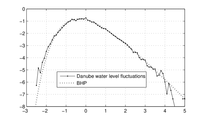
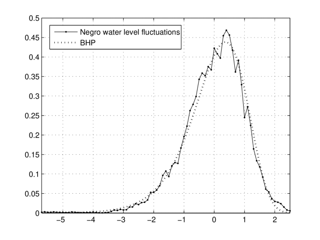
Jánosi and Gallas [7] analyzed statistics of the Alpine river Danube daily water level collected, over the period 1901-97, at Nagymaros, Hungary. The authors found, in the one day logarithmic rate of change of the river water level, similar characteristics to those of company growth (see Stanley et al. [8]) which shows that the properties seen in company data are present in a wider class of complex systems. Bramwell et al. [3] defined a daily water level mean and variance and computed the daily river water level fluctuations. They have shown a data collapse of the Danube daily water level fluctuations histogram to the (reversed) Bramwell-Holdsworth-Pinton (BHP) probability density function (pdf). Dahlstedt and Jensen [6] described the statistical properties of several river systems. They did a careful study of the size of basin areas influence in the data collapse of the rivers water level and runoff, in particular of river Negro at Manaus, to the reversed BHP and to the Gaussian pdf showing that not all rivers have the same statistical behavior. In this paper, we study, again, the South American river Negro daily water level at Manaus (104 years). We compute and present a cyclic fit for the Negro daily water level period and the Negro daily water level standard deviation. We show that the histogram of the Danube water level fluctuations is on top of the reversed BHP pdf, which does not happen for the Negro daily water level.
2 BHP and the Danube and Negro data
We define the Danube daily water level period by
| (1) |
where is the number of observed years and is the Danube daily water level time series.111All the observations of the days of February were eliminated.
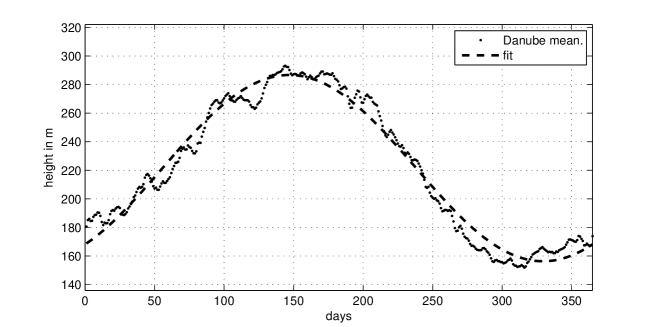
In Figure 1, we show a fit to the Danube daily water level period . The mean period fit, using the first harmonic of the Fourier series, is given by
| (2) |
The percentage of variance explained by the fit is .
We define the Negro daily water level period by
| (3) |
where is the number of observed years and is the Negro daily water level time series. 222All the observations of the days of February were eliminated.
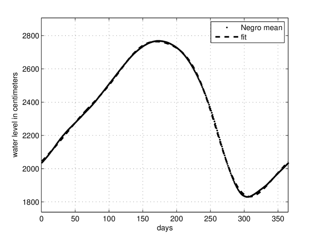
In Figure 2, we show a fit of the Negro daily water level period . The mean period fit, using the first four sub-harmonics of the Fourier series, is given by
| (4) |
where and are given in table 1. The percentage of variance explained by the fit is .
We define the Danube daily water level standard deviation by
| (5) |
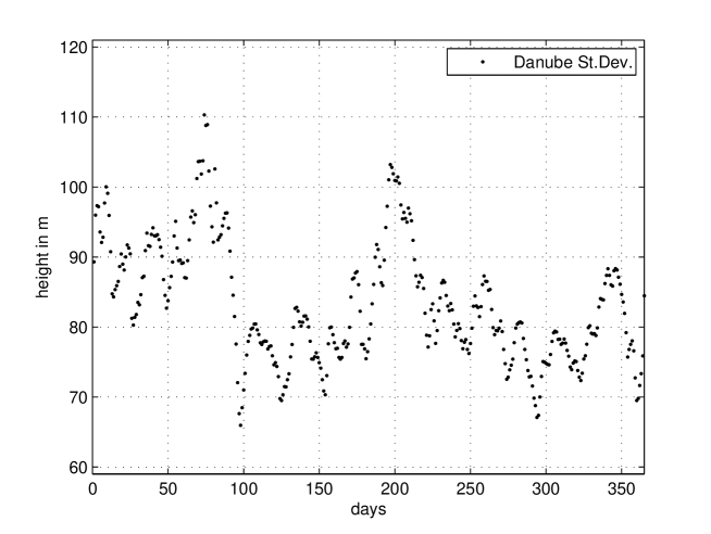
In Figure 3, we show the chronogram of the Danube daily water level standard deviation.
We define the Negro daily water level standard deviation given by
| (6) |
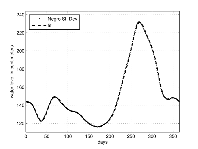
In Figure 4, we show a fit of the Negro daily water level standard deviation. The fit , using the first ten sub-harmonics of the Fourier series, is given by
| (7) |
where and are given in table 2. The percentage of variance explained by the fit is .
Following Bramwell et. al [3], we define the Danube daily water level fluctuations by
| (8) |
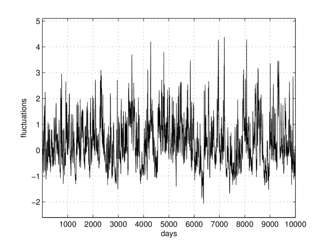
In Figure 5, we show the Danube daily water level fluctuations . As shown by Bramwell et al. [3], the (reversed) BHP pdf falls on top of the histogram of the Danube daily water level fluctuations, in the semi-log scale (see Figure 6).
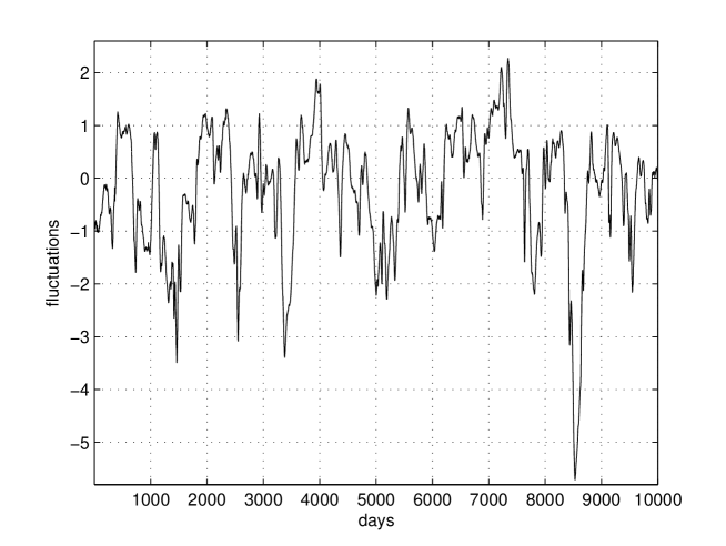
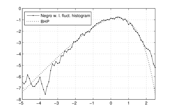
We define the Negro daily water level fluctuations by
| (9) |
3 Conclusions
We computed and presented a cyclic fit for the Negro daily water level period and for the Negro daily water level standard deviation using the first four and ten sub-harmonics, respectively. We computed the histogram of the Negro daily water level fluctuations at Manaus, and we compared it with the BHP pdf. The histogram of the Negro daily water level fluctuations is close to the BHP pdf. We have shown that the histogram of the Danube water level fluctuations is on top of the reversed BHP pdf, which does not happen for the river Negro daily water level fluctuations.
Acknowledgements
We thank Imre Jánosi for providing the river Danube data and Mrs. Andrelina Santos of the Agência Nacional de Águas of Brazil for providing the river Negro data.
References
- [1] Bramwell, S.T., Christensen, K., Fortin, J.Y., Holdsworth, P.C.W., Jensen, H.J., Lise, S., López, J.M., Nicodemi, M. & Sellitto,M. (2000) Universal Fluctuations in Correlated Systems, Phys. Rev. Lett. 84, 3744–3747.
- [2] Bramwell, S.T., Fortin, J.Y., Holdsworth, P.C.W., Peysson, S., Pinton, J.F., Portelli, B. & Sellitto,M. (2001) Magnetic Fluctuations in the classical XY model: the origin of an exponential tail in a complex system, Phys. Rev E 63, 041106.
- [3] Bramwell, S.T., Fennell, T., Holdsworth, P.C.W., & Portelli, B. (2002) Universal Fluctuations of the Danube Water Level: a Link with Turbulence, Criticality and Company Growth, Europhysics Letters 57, 310.
- [4] Bramwell, S.T., Holdsworth, P.C.W., & Pinton, J.F. (1998) Universality of rare fluctuations in turbulence and critical phenomena, Nature 396, 552–554.
- [5] Dahlstedt, K., & Jensen, H.J. (2001) Universal fluctuations and extreme-value statistics, J. Phys. A: Math. Gen. 34, 11193–11200.
- [6] Dahlstedt, K., & Jensen, H.J. (2005) Fluctuation spectrum and size scaling of river flow and level, Physica A 348, 596–610.
- [7] Jánosi, I.M., & Gallas, J.A.C. (1999) Growth of companies and water-level fluctuations of the River Danube, Physica A 271, 448–457.
- [8] Stanley, M.H.R., Amaral, L. A. N., Buildrev, S. V., Havlin, S., Leschhorn, H. Maass, P., Salinger, M.A. & Stanley, E. (1996) Scaling behaviour in the growth of companies. Letters to Nature 379, 29, 804-806.
| n | ||
|---|---|---|
| 0 | 4671.2 | - |
| 1 | -386.92 | 195.28 |
| 2 | 73.672 | 74.577 |
| 3 | 29.0336 | -12.473 |
| 4 | -9.9726 | -13.724 |
| n | ||
|---|---|---|
| 0 | 304.1 | - |
| 1 | -8.505 | 33.983 |
| 2 | -28.086 | 1.1481 |
| 3 | -2.6941 | -8.1938 |
| 4 | 6.5597 | -1.9674 |
| 5 | -3.6529 | 1.6374 |
| 6 | 2.1779 | 1.2313 |
| 7 | -0.2847 | -1.2559 |
| 8 | -0.5713 | -0.6129 |
| 9 | 1.7276 | 0.54441 |
| 10 | -1.0358 | 0.64293 |