Model-independent description of $B\to\pi l\nu$ decays and a determination of $|V_{ub}|$

Abstract

We propose a new parametrization of the $B\to\pi$ vector form factor, $f_{+}(q^{2})$, as an expansion in powers of a conformal mapping variable, which satisfies unitarity, analyticity and perturbative QCD scaling. The unitarity constraint is used also for defining the systematic error of the expansion. We fit with the new parametrization the available experimental and theoretical information on exclusive $B\to\pi l\nu$ decays, making a conservative estimate of the effects of correlations in the systematic and statistical errors of the lattice results. With four parameters to describe $f_{+}(q^{2})$, the systematic error is negligible in the whole semileptonic region. We also obtain $|V_{ub}|=(3.54\pm 0.30)\times 10^{-3}$ where, in our approach, the uncertainty is predominantly statistical.

I Introduction

As shown recently [1, 2, 3, 4], the extraction of $|V_{ub}|$ from the exclusive semileptonic $B\to\pi$ decays has become competitive with determinations from inclusive decays. The exclusive decay approach requires the theoretical description of the matrix element

$$\langle\pi(p_{\pi})|\bar{u}\gamma_{\mu}b|B(p_{\pi}+q)\rangle \!\!\!\!=$$ (1)

$$\left(2p_{\pi\mu}+q_{\mu}-q_{\mu}\frac{m_{B}^{2}-m_{\pi}^{2}}{q^{2}}\right)f_{+}(q^{2})$$

$$+\,q_{\mu}\frac{m_{B}^{2}-m_{\pi}^{2}}{q^{2}}f_{0}(q^{2}),$$

where $q$ is the momentum of the lepton pair and $f_{+}(q^{2})$ and $f_{0}(q^{2})$ denote the vector and scalar form factors, respectively. For light leptons, $l=e,\mu$, only the vector form factor contributes to the spectrum

$$\frac{d\Gamma}{dq^{2}}(\bar{B}^{0}\to\pi^{+}l^{-}\bar{\nu}_{\ell})=\frac{G_{F}^{2}|V_{ub}|^{2}}{192\pi^{3}m_{B}^{3}}\,\lambda^{3/2}(q^{2})|f_{+}(q^{2})|^{2},$$ (2)

where $\lambda(q^{2})=(m_{B}^{2}+m_{\pi}^{2}-q^{2})^{2}-4m_{B}^{2}m_{\pi}^{2}$ is $4m_{B}^{2}$ times the pion three-momentum squared in the $B$-meson rest frame. The physical range of semileptonic decays is $0\leq q^{2}\leq t_{-}$, with $t_{-}=(m_{B^{0}}-m_{\pi^{+}})^{2}=26.42\,\mbox{GeV}^{2}$.

The $q^{2}$-spectrum of $B\to\pi\ell\nu$ decays has been measured with increasing precision by the CLEO [5, 6], Belle [7], and BaBar collaborations [8, 9]. The accuracy of theoretical calculations of the form factors is also continuously improving. The calculations are based either on QCD light-cone sum-rules (LCSR), which provide reliable determinations at small $q^{2}$ [10, 11, 12], or on lattice simulations, which give accurate results at larger values of $q^{2}$ [13, 14, 15, 16, 17, 18].

From general principles of quantum field theory it is known that the vector form factor $f_{+}(q^{2})$ is a real analytic function in the complex $q^{2}$-plane cut for $q^{2}\geq t_{+}$, where $\sqrt{t_{+}}=(m_{B^{0}}+m_{\pi^{+}})=5.419\,\mbox{GeV}$ is the $B\pi$ threshold. Angular momentum conservation imposes the behavior $\mbox{Im}\,f_{+}(q^{2})\sim(q^{2}-t_{+})^{3/2}$ near the threshold. In addition, $f_{+}(q^{2})$ has a pole below the branch point, at $q^{2}=m_{B^{*}}^{2}$ ($m_{B^{*}}=5.325\,\mbox{GeV}$). As shown in [19], unitarity applied to a certain QCD correlator provides a constraint on the magnitude of $f_{+}(q^{2})$ along the cut, while scaling in perturbative QCD requires a power-law fall-off, like $1/q^{2}$, up to logarithmic corrections [20, 21].

To maximize the usefulness of this information about $B\to\pi\ell\nu$ decays and, for instance, determine $|V_{ub}|$, it is crucial to have a parametrization of $f_{+}(q^{2})$, which satisfies the above theoretical requirements, and whose associated systematic error is quantifiable and small compared to experimental and other theoretical errors. The purpose of the present work is to provide such a parametrization. In Sec. II, we discuss the recent models proposed in the literature, and show that they do not satisfy all of the constraints mentioned above. In Sec. III, we propose a simple analytic parametrization of $f_{+}(q^{2})$, which combines the pole factorization with an expansion in powers of a conformal mapping variable, and in Sec. IV, we express the unitarity constraints in terms of the coefficients of this expansion. By fitting the experimental differential decay rate $B\to\pi l\nu$ and the values of $f_{+}(q^{2})$ calculated from LCSR and the lattice, we obtain in Sec. VIII a model-independent representation of the form factor $f_{+}(q^{2})$ in the physical region. The procedure also yields a precise value of $|V_{ub}|$, given in Sec. IX.

II Recent parametrizations of the form factor

A comparison of the various parametrizations proposed in the literature was done recently in [22]. As shown there, the simple expressions with a pole at $q^{2}=m_{B^{*}}^{2}$, proposed in [11, 23], cannot provide an accurate description of the form factor in the whole physical domain. Thus, more systematic expansions, which incorporate the constraints of analyticity and unitarity, have been considered.

A first type of parametrization is inspired by the technique of unitarity bounds proposed by Okubo [24, 25] and applied subsequently to various semileptonic form factors [26, 27, 28]. They are obtained by exploiting the analyticity and positivity properties of vacuum polarization functions of the type $\Pi_{\mu\nu}(q){=}i\int d^{4}xe^{iq\cdot x}$ $\langle 0|T\{J_{\mu}(x)$ $J_{\nu}^{\dagger}(0)\}|0\rangle$, where $J_{\mu}=\bar{u}\gamma^{\mu}b$ here. In this approach, the form factor can be expanded as [29, 1]

$$f_{+}(q^{2})=\frac{1}{B(q^{2})\phi(q^{2},t_{0})}\,\sum\limits_{n\geq 0}a_{n}(t_{0})z^{n}\,,$$ (3)

where $a_{n}(t_{0})$ are real coefficients and $z\equiv z(q^{2},t_{0})$ is the function

$$z(q^{2},t_{0})=\frac{\sqrt{t_{+}-q^{2}}-\sqrt{t_{+}-t_{0}}}{\sqrt{t_{+}-q^{2}}+\sqrt{t_{+}-t_{0}}},$$ (4)

which maps the $q^{2}$-plane cut for $q^{2}\geq t_{+}$ onto the disk $|z(q^{2},t_{0})|<1$ in the $z$ complex plane, such that $z(t_{+},t_{0})=-1$ and $z(\infty,t_{0})=1$. The parameter $t_{0}<t_{+}$, which is arbitrary, determines the point $q^{2}$ mapped onto the origin in the $z$ plane, i.e. $z(t_{0},t_{0})=0$.

The function $B(q^{2})$ is the Blaschke factor

$$B(q^{2})=\frac{z(q^{2},t_{0})-z(m_{B^{*}}^{2},t_{0})}{1-z(q^{2},t_{0})z(m_{B^{*}}^{2},t_{0})}=z(q^{2},m_{B^{*}}^{2})\,,$$ (5)

which accounts for the pole at $q^{2}=m_{B^{*}}^{2}$. By construction $|B(q^{2})|=1$ for $q^{2}\geq t_{+}$.

The last factor in (3), the outer function $\phi(q^{2},t_{0})$, has the expression

$$\phi(q^{2},t_{0})= \!\!\!\!\sqrt{\frac{1}{32\pi\chi_{1^{-}}(0)}}(\sqrt{t_{+}-q^{2}}+\sqrt{t_{+}-t_{0}})$$ (6)

$$\times \!\!\frac{t_{+}-q^{2}}{(t_{+}-t_{0})^{1/4}}\times(\sqrt{t_{+}-q^{2}}+\sqrt{t_{+}})^{-5}$$

$$\times \!\!(\sqrt{t_{+}-q^{2}}+\sqrt{t_{+}-t_{-}})^{3/2},$$

where $\chi_{1^{-}}(0)$ is the derivative of the transverse component of the polarization function $\Pi_{\mu\nu}(q)$ at the Euclidean momentum $Q^{2}=-q^{2}=0$ [19]. Because of the large value of the $b$-quark mass, this quantity can be computed by means of perturbative QCD and the operator product expansion [30, 19]. On the other hand, the spectral function associated with $\Pi_{\mu\nu}(q)$ is a sum of positive contributions. Thus, if we assume that it is saturated by $B\pi$ intermediate states, unitarity and crossing symmetry guarantee that the coefficients $a_{n}(t_{0})$ satisfy the inequality

$$\sum\limits_{n=0}^{\infty}a_{n}^{2}(t_{0})\leq 1\,.$$ (7)

This allows one to calculate bounds on the values of the form factor or its derivatives at points inside the analyticity domain, in particular in the physical region. For the $B\to\pi$ form factors, such bounds were investigated in [1] and [19].

The expression (3) was also adopted as a parametrization of the form factor in [31, 32, 22]. In this case the expansion is truncated at a finite order. However, as noticed in [33], the form factor increases then like $f_{+}(q^{2})\sim(q^{2})^{1/4}$ at large $|q^{2}|$, in contradiction with perturbative QCD scaling. This behavior follows from the expression (6) for the outer function, taking into account that all the other factors in Eq. (3) are finite at $|q^{2}|\to\infty$. Moreover, when the series is truncated, the expression (3) has an unphysical singularity at the $B\pi$ production threshold $t_{+}$, produced by the factor $(t_{+}-q^{2})$ in the numerator of Eq. (6). This unphysical singularity may distort the behavior near the upper end of the physical region, where the form factor is poorly known.

It should be noted that in the calculation of bounds one uses the full expansion in Eq. (3), with an infinite number of terms. Then the series cancels the zeros of the function $\phi(q^{2},t_{0})$ at $q^{2}=t_{+}$ and at $q^{2}\to\infty$, restoring the required properties of $f_{+}(q^{2})$. Actually, it can be shown that imposing the condition that the series vanishes at threshold or at infinity does not change the unitarity bounds (this answers a question raised in [33] about the possibility of improving the bounds in this way).

A second type of parametrization, used recently for the $B\to\pi$ form factors in [2, 4], is based on the Omnès representation [34], which expresses an analytic function in terms of its phase along the boundary of the analyticity domain. If the phase $\delta(t)$, defined by $f_{+}(t+i\epsilon)=|f_{+}(t)|\exp(i\delta(t))$ for $t\geq t_{+}$, has a finite limit at infinity, the Omnès representation requires only one subtraction. Taking into account the pole at $q^{2}=m_{B^{*}}^{2}$ and assuming, as in [2], that the form factor does not have zeros in the complex plane, the representation reads

$$f_{+}(q^{2})=\!\! f \!\!\!\!{}_{+}(q_{1}^{2})\,\frac{m_{B^{*}}^{2}-q_{1}^{2}}{m_{B^{*}}^{2}-q^{2}}\exp\left[\frac{q^{2}-q^{2}_{1}}{\pi}\right.$$ (8)

$$\times \!\!\left.\int\limits_{t_{+}}^{\infty}\frac{\delta(t)\,\mbox{d}t}{(t-q^{2}_{1})(t-q^{2})}\,\right],$$

where $q_{1}^{2}$ is an arbitrary subtraction point. By Watson’s theorem [35], the phase $\delta(t)$ is equal, below the first inelastic threshold, to the phase of the $P$-wave with $I=1/2$ of the $\pi B\to\pi B$ elastic scattering. Since this phase is not known, in Refs. [2, 4] the contribution of the integral was suppressed by using a multiply-subtracted dispersion relation. Neglecting altogether the dispersion integral, the form factor is represented in [4] as

$$f_{+}(q^{2})=\frac{1}{m_{B^{*}}^{2}-q^{2}}\prod\limits_{j=1}^{n}[f_{+}(q^{2}_{j})(m_{B^{*}}^{2}-q^{2}_{j})]^{\alpha_{j}(q^{2})},$$ (9)

where

$$\alpha_{j}(q^{2})=\prod\limits_{i=0,i\neq j}^{n}\frac{q^{2}-q^{2}_{i}}{q^{2}_{j}-q^{2}_{i}}\,.$$ (10)

However, it is easy to see that the expression (9) defines an entire function in the complex $q^{2}$-plane, with no cut for $q^{2}\geq t_{+}$. So, this parametrization does not have the proper structure of the physical form factor required by analyticity and unitarity. Moreover, the expression (9) exhibits at $|q^{2}|\to\infty$ an exponential behavior like $\exp[C(q^{2})^{n-1}]$, where $C$ is a combination of the values $f_{+}(q^{2}_{j})$. This anomalous behavior follows from the multiple subtraction of a dispersion relation that requires in general only one subtraction. The values $f_{+}(q^{2}_{j})$ for $j>1$ are not independent: according to (8), they can all be expressed in terms of $f_{+}(q^{2}_{1})$ and the dispersion integral. By taking into account these relations in the multiply-subtracted dispersion relation, one recovers the original relation (8). However, if the values $f_{+}(q^{2}_{j})$ are treated as independent, the form factor behaves as an exponential at large $q^{2}$, in contradiction with QCD scaling.

Though the shortcomings discussed in this section formally concern the behavior of the parametrizations of Eqs. (3) and (9) outside the semileptonic domain, it is important to construct a representation of the form factor which has the correct analyticity properties in the whole complex plane. Besides the obvious argument that a parametrization that does not satisfy these properties cannot describe the form factor correctly, the introduction of unpysical singularities, sometimes close to the semileptonic domain, can distort the form factor in that region. Given the levels of precision currently reached and expected in the study of exclusive $B\to\pi$ decays, such distortions are unacceptable.

III A new parametrization for $f_{+}(q^{2})$

We start by the remark that the product $(1-q^{2}/m_{B^{*}}^{2})f_{+}(q^{2})$ is analytic in the complex $q^{2}$-plane cut along the real axis for $q^{2}\geq t_{+}$ and is finite for $q^{2}\to\infty$, due to the scaling behavior $f_{+}(q^{2})\sim 1/q^{2}$. An expansion of the product that converges in the whole complex plane is obtained in terms of a variable that conformally maps the cut $q^{2}$ plane onto a disk [36, 37]. The variable $z=z(q^{2},t_{0})$ defined in Eq. (4) performs precisely this mapping. Thus, we propose the simple parametrization

$$f_{+}(q^{2})=\frac{1}{1-q^{2}/m_{B^{*}}^{2}}\,\sum\limits_{k=0}^{K}b_{k}(t_{0})\,z^{k}\,.$$ (11)

The polynomial in powers of $z$ displays the branch point at $q^{2}=t_{+}$ and is finite in the disk $|z|\leq 1$, i.e. in the whole $q^{2}$-plane. This ensures the correct analytic structure in the complex plane and the proper scaling, $f_{+}(q^{2})\sim 1/q^{2}$ at large $q^{2}$.

As mentioned in the Introduction, $f_{+}(q^{2})$ must satisfy also the condition $\mbox{Im}\,f_{+}(q^{2})\sim(q^{2}-t_{+})^{3/2}$ near $t_{+}$. Also, analyticity implies that near threshold $\mbox{Re}\,f_{+}(q^{2})\sim a_{+}+b_{+}(q^{2}-t_{+})+\ldots$, where $a_{+}$ and $b_{+}$ are constants. We recall that from the definition (4) of the variable $z=z(q^{2},t_{0})$ it follows that the threshold $t_{+}$ is mapped onto the point $z=-1$, and $(z+1)\sim{\rm const.}\times(q^{2}-t_{+})^{1/2}$ near $z=-1$. Then, it is easy to see that $f_{+}$ must satisfy the condition

$$\left[\frac{{\rm d}f_{+}}{{\rm d}z}\right]_{z=-1}=0,$$ (12)

which, written in terms of the coefficients $b_{k}$ appearing in (11), takes the simple form

$$\sum_{k=1}^{K}(-1)^{k+1}\,k\,b_{k}(t_{0})=0.$$ (13)

By inserting in Eq. (11) the solution of (13), written as

$$b_{K}=-\frac{(-1)^{K}}{K}\sum\limits_{k=0}^{K-1}(-1)^{k}kb_{k},$$ (14)

we arrive at the expression

$$f_{+}(q^{2})=\frac{1}{1-q^{2}/m_{B^{*}}^{2}}\,\sum\limits_{k=0}^{K-1}b_{k}\left[z^{k}-(-1)^{k-K}\frac{k}{K}\,z^{K}\right],$$ (15)

where $z=z(q^{2},t_{0})$. This is the parametrization that we investigate in the present work.

As concerns the conformal mapping, i.e. the parameter $t_{0}$ in (4), it was remarked in [31, 32] that for $t_{0}=t_{opt}$ with

$$t_{opt}\equiv(m_{B}+m_{\pi})(\sqrt{m_{B}}-\sqrt{m_{\pi}})^{2}=20.062\,\mbox{GeV}^{2}\ ,$$ (16)

the semileptonic domain is mapped onto the symmetric interval $|z|\leq 0.279$ in the $z$-plane. As we shall discuss below, this choice minimizes the maximum truncation error in the semileptonic domain. An additional argument for this choice is provided by the general theory of the representation of data distributed along an interval: as shown in [37], in this case the optimal expansion of the function is obtained by using a complete set of orthogonal polynomials of the variable that maps the original complex cut plane onto an ellipse, such that the cut becomes the boundary and the physical range is mapped onto the interval situated between the focal points. We checked that the optimal ellipse given in [37] is in our case very close to the circle $|z(q^{2},t_{opt})|=1$.

Other choices of $t_{0}$ are useful if one is interested in having a more accurate description in a specific energy range. Two values, $t_{0}=0$ and $t_{0}=t_{-}$ were investigated in [22]. In our analysis we shall adopt the choice $t_{0}=t_{opt}$, with $t_{opt}$ given in (16).

IV Unitarity constraint

The unitarity condition (7) can also be expressed in terms of the coefficients $b_{k}(t_{0})$. By comparing the representations in Eqs. (3) and (11) we have

$$\sum\limits_{n=0}^{\infty}a_{n}(t_{0})z^{n}=\Psi(z)\sum\limits_{k=0}^{K}b_{k}(t_{0})z^{k}\,,$$ (17)

where $\Psi(z)$ is a known function

$$\Psi(z)=\frac{m_{B^{*}}^{2}}{4(t_{+}-t_{0})}\,\Phi(z)\,\frac{(1-z)^{2}(1-z_{*})^{2}}{(1-zz_{*})^{2}}.$$ (18)

We denote by $z_{*}=z(m_{B^{*}}^{2},t_{0})$ the position of the pole in the variable $z$, and $\Phi(z)\equiv\phi(q^{2}(z),t_{0})$ is the outer function expressed in terms of $z$, by using the inverse of Eq. (4)

$$q^{2}(z)=t_{+}-(t_{+}-t_{0})\,\left(\frac{1+z}{1-z}\right)^{2}\,.$$ (19)

The function $\Psi(z)$, which depends also on the parameter $t_{0}$, is analytic in $|z|<1$. Thus, we can expand it around $z=0$ as

$$\Psi(z)=\sum\limits_{k=0}^{\infty}\eta_{k}(t_{0})z^{k}.$$ (20)

Inserting this expansion in (17), we obtain

$$a_{n}(t_{0})=\sum\limits_{k=0}^{\min[K,n]}\eta_{n-k}(t_{0})b_{k}(t_{0}),\quad\quad n\geq 0.$$ (21)

Then the inequality (7), expressed in terms of the coefficients $b_{j}(t_{0})$, reads as

$$\sum\limits\limits_{j,k=0}^{K}B_{jk}(t_{0})b_{j}(t_{0})b_{k}(t_{0})\leq 1,$$ (22)

where

$$B_{jk}(t_{0})=\sum\limits_{n=0}^{\infty}\eta_{n}(t_{0})\eta_{n+|j-k|}(t_{0}).$$ (23)

From Eqs. (6) and (18) it follows that the function $\Psi(z)$ is bounded in the closed disk $|z|\leq 1$, so its Taylor coefficients $\eta_{j}$ are rapidly decreasing. Therefore, the coefficients $B_{jk}(t_{0})$ can be computed by performing in (23) the summation upon $n$ up to a finite order, about 100 in practice.

As discussed in [33], the leading contributions to the sum over the coefficients $a_{n}^{2}$, which appears in the unitarity condition (7), are of order $(\Lambda/m_{b})^{3}$ in the heavy $b$-quark expansion. Thus, we expect that the 1 appearing on the right-hand sides of the constraints of Eqs. (7) and (22) is a significant overestimate, the real bound being more realistically on the order of a few per mil. Were we to consider these more stringent bounds in the sequel, we would be able to reduce the number of terms kept in the series expansion of the form factor. This would significantly reduce the systematic uncertainty that we encounter when using this expansion to extrapolate the form factor to regions where it is not constrained by the input that we use. However, in the absence of a more precise quantitative argument for strengthening the bound, we choose to keep Eq. (22) as it stands. In any event, if and when such an argument is found, the procedures explained in the following sections can be carried over as is, simply replacing the right-hand side of the inequality (22) by the relevant smaller number.

For the numerical evaluation of the coefficients $B_{jk}$ we need the value of $\chi_{1^{-}}(0)$ entering the outer function (6). Perturbative QCD and the operator product expansion give  [30, 19]

$$\chi_{1^{-}}(0)=\frac{3[1+1.14\,\alpha_{s}(\bar{m}_{b})]}{32\pi^{2}m_{b}^{2}}-\frac{\bar{m}_{b}\langle\bar{u}u\rangle}{m_{b}^{6}}-\frac{\langle\alpha_{s}G^{2}\rangle}{12\pi m_{b}^{6}}\ ,$$ (24)

where $m_{b}=4.9\,\mbox{GeV}$ is the pole mass and $\bar{m}_{b}$ the $\overline{\mbox{MS}}$ mass, with $\bar{m}_{b}(2\,\mbox{GeV})\approx 4.98$ GeV, obtained from $\bar{m}_{b}(\bar{m}_{b})\approx 4.2$ GeV [38] and the four-loop running in the $\overline{\mbox{MS}}$ scheme [39]. We took $\alpha_{s}(\bar{m}_{b})=0.22$ [38]. The gluon condensate has the standard value $\langle\alpha_{s}G^{2}\rangle=0.038\,\mbox{GeV}^{4}$ given in [40], while for the quark condensate we used the two-flavor value $\langle\bar{u}u\rangle\approx-(278\,\,\mbox{MeV})^{3}$ in the $\overline{\mbox{MS}}$ scheme at scale 2 GeV [41]. From the above values we derive $\bar{m}_{b}\,\langle\bar{u}u\rangle\approx-0.107\ \mbox{GeV}^{4}$ at scale 2 GeV, and we adopt this value also at scale $m_{b}$, since the scale dependent corrections to the product are negligible. By inserting in (24) the above central values we obtain $\chi_{1^{-}}(0)\approx 5.01\times 10^{-4}$. For illustration, we give in Table 1 the coefficients $B_{jk}(t_{0})$ calculated with this value of $\chi_{1^{-}}(0)$ for $K=5$ and several values of $t_{0}$.

We mention also that when $K\to\infty$, the expansion in Eq. (11) is convergent in the whole disk $|z|<1$, i.e. in the whole $q^{2}$-plane cut along the real axis for $q^{2}\geq t_{+}$. Moreover, the unitarity condition (22) can be used to derive an explicit upper bound on the truncation error. We present the derivation of this bound in the Appendix.

Table 1: The matrix elements, $B_{jk}(t_{0})$, which enter the unitarity bound (22) for $K=5$ and several values of $t_{0}$. The remaining coefficients are obtained from the relations $B_{j(j+k)}=B_{0k}$ and the symmetry property $B_{jk}=B_{kj}$, obvious from Eq. (23).

$t_{0}$(${\rm GeV^{2}}$)	$B_{00}$	$B_{01}$	$B_{02}$	$B_{04}$	$B_{04}$	$B_{05}$
0	0.0197	-0.0049	-0.0108	0.0057	0.0006	-0.0005
$t_{opt}$	0.0197	0.0042	-0.0109	-0.0059	-0.0002	0.0012
$t_{-}$	0.0197	0.0118	-0.0015	-0.0078	-0.0077	-0.0053

V Theoretical and experimental input

At low $q^{2}$, the form factor is calculated in the framework of LCSR [10, 11, 12]. We use $f_{\mathrm{LCSR}}\equiv f_{+}(0)=0.26$, with the uncertainty $\delta f_{\mathrm{LCSR}}=0.03$ [22]. Lattice calculations provide the value of the form factor at eight additional $q^{2}$-points: three are taken from FNAL-MILC [13, 16] and five from HPQCD, updated in [17]. As in [2, 4], we take the three FNAL-MILC results from [1]. 

The available experimental data consist in the partial branching fractions over bins in $q^{2}$. We use 10 data from the tagged analyses (4 bins from CLEO [6], which replace the older data [5], 3 from Belle [7], and 3 from BaBar [8]), and 12 bins from the untagged BaBar analysis [9], where the full covariance matrix is available. The total number of data points from theory and experiment is 31.

It is convenient to define the global $\chi^{2}$

$$\chi^{2}(b_{k},|V_{ub}|)=\chi^{2}_{th}+\chi^{2}_{exp}\,,$$ (25)

where

$$\chi^{2}_{th}=\sum\limits_{j,k=1}^{8}[f_{j}^{in}-f_{+}(q^{2}_{j})]C^{-1}_{jk}[f_{k}^{in}-f_{+}(q^{2}_{k})]$$

$$~{}~{}~{}~{}~{}~{}~{}+(f_{+}(0)-f_{\mathrm{LCSR}})^{2}/(\delta f_{\mathrm{LCSR}})^{2}\,,$$

$$\chi^{2}_{exp}=\sum\limits_{j,k=1}^{22}[{\mathcal{B}}_{j}^{in}-{\mathcal{B}}_{j}(f_{+})]C^{-1}_{{\mathcal{B}}\,jk}[{\mathcal{B}}_{k}^{in}-{\mathcal{B}}_{k}(f_{+})]\,.$$ (26)

In the above relations, the $f_{j}^{in}$ denote the values of the form factor calculated on the lattice at the points $q^{2}_{j}$; ${\mathcal{B}}_{j}^{in}$ are the experimental partial branching fractions and ${\mathcal{B}}_{j}(f_{+})$ the values calculated by integrating Eq. (2) over the bins $[q^{2}_{j},q^{2}_{j+1}]$, with a given parametrization for the form factor $f_{+}(q^{2})$. To convert to a rate, we use the $B^{0}$ lifetime, $\tau_{B}^{0}=1/\Gamma_{\rm tot}=(1.527\pm 0.008)\times 10^{-12}s$ [42].

The covariance matrices $C$ and $C_{B}$ are written formally: in practice they are block diagonal, with independent blocks for each independent set of experimental data or lattice results. Unfortunately, the covariance matrices are not provided for the lattice calculations. Thus, we make here a set of reasonable assumptions on the possible correlations based on the information provided in the papers and on our experience with such calculations. The lattice results of [13, 16] and [17] are obtained using different discretizations for the heavy quark, but on subsets of the MILC, $N_{f}=2+1$, gauge configurations which have significant overlap. Thus, in addition to assuming that the statistical errors on $f_{+}(q^{2})$ at different $q^{2}$ within each calculation have a 50% correlation, we assume that there is a 25% correlation between the errors in the two calculations. Such correlations in the statistical errors have been assumed to be negligible in previous work [1, 2, 3, 4]. Regarding the systematic errors, since the heavy-quark discretizations and methods used are different, we assume negligible correlations in the systematic errors between the two calculations, but given their nature, assume 100% correlations within each simulation. Though these assumptions cannot replace covariance matrices determined by the lattice collaborations themselves, we believe that they are reasonable and will not lead to underestimated errors. We have verified that without these correlations, for instance, the results for $f_{+}$ versus $q^{2}$ quoted below would have fit errors reduced by up to 30%.

VI Results of the fits

We performed a combined fit of the above input by minimizing $\chi^{2}$ defined in (25), using the representation of $f_{+}(q^{2})$ given in (15), with $z=z(q^{2},t_{opt})$. The free parameters are $|V_{ub}|$ and the real coefficients $b_{k}$, $k\leq K-1$ subject to the unitarity constraint (22), with $b_{K}$ given by the expression (14). The total number of parameters is $N=K+1$.

According to convex optimization theory [43], the optimum values $b_{k}^{(0)}$ and the optimal Lagrange multiplier $\lambda_{0}$ minimizing the Lagrangian

$${\cal L}(b_{j},|V_{ub}|)=\chi^{2}(b_{j},|V_{ub}|)+\lambda\left(\sum\limits\limits_{j,k=0}^{K}B_{jk}b_{j}b_{k}-1\right)\,,$$ (27)

satisfy the alignment condition

$$\lambda_{0}\left(\sum\limits\limits_{j,k=0}^{K}B_{jk}b_{j}^{(0)}b_{k}^{(0)}-1\right)=0.$$ (28)

Therefore, either $\lambda_{0}=0$ and the optimal parameters $b_{k}^{(0)}$ of the unconstrained minimum of $\chi^{2}(b_{k},|V_{ub}|)$ satisfy automatically the constraint (22), or $\lambda_{0}\neq 0$, when the optimal parameters saturate the constraint (22).

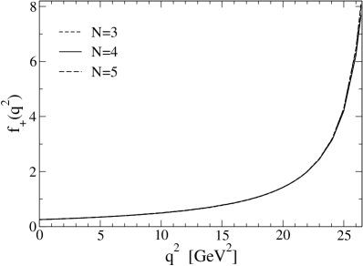
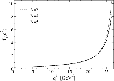
Figure 1: Left: the form factor $f_{+}(q^{2})$ computed with the new representation (15) and the parameters from (29)-(VI). Right: the form factor calculated with the traditional parametrization (3) and the parameters from (32)-(VI).

A nontrivial form factor is obtained for $K\geq 2$, i.e. a total number of parameters, $N\geq 3$. The results of the fits obtained by increasing $N$ are presented below:

$$N=3; K=2;\quad\chi^{2}=21.17,\quad\chi^{2}/dof=0.76,$$ (29)

$$b_{0}=0.420\pm 0.031,\quad b_{1}=-0.514\pm 0.070,$$

$$\quad\quad|V_{ub}|=(3.58\pm 0.27)\times 10^{-3},$$

$$N=4;\quad\quad K=3;\quad\quad\chi^{2}=21.03,$$

$$\chi^{2}/dof=0.78,\quad\quad b_{0}=0.421\pm 0.031,$$

$$b_{1}=-0.476\pm 0.122,\quad\quad b_{2}=-0.399\pm 0.381,$$

$$\hskip 28.45274pt|V_{ub}|=(3.57\pm 0.27)\times 10^{-3},$$ (30)

$$\quad\quad N=5;\quad\quad K=4;\quad\quad\chi^{2}=21.00,$$

$$\quad\chi^{2}/dof=0.81,\quad b_{0}=0.421\pm 0.031,$$ (31)

$$b_{1}=-0.469\pm 0.129,\quad b_{2}=-0.178\,^{+1.358}_{-1.313}\,,$$

$$b_{3}=-0.825\,^{+4.067}_{-4.042}\,,\quad|V_{ub}|=(3.54\pm 0.30)\times 10^{-3}.$$

For simplicity we omitted the upper index “(0)” in the notation of the optimal parameters. All the errors indicated are statistical. We mention that for the fits (29) and (VI) the unitarity constraint (22) is not saturated, while the slightly asymmetric errors on the coefficients $b_{2}$ and $b_{3}$ in (VI) are produced mainly by this constraint.

The form factor calculated with the central values of the parameters from (29)-(VI) is plotted in the left panel of Fig. 1. For comparison we repeat the analysis also with the standard parametrization (3). We recall that this parametrization has an unphysical singularity at threshold, and we cannot impose the threshold condition that we use above. Therefore, for a certain $K$ there are $K+1$ parameters $a_{k}$, constrained by the unitarity condition (7), and the total number of parameters is $N=K+2$. The best fits for the lowest values of $N$ are

$$N=3; K=1;\quad\chi^{2}=27.68,\quad\chi^{2}/dof=0.98,$$ (32)

$$a_{0}=0.024\pm 0.002,\quad a_{1}=-0.033\pm 0.004,$$

$$\quad\quad|V_{ub}|=(3.63\pm 0.28)\times 10^{-3},$$

$$N=4;\quad\quad K=2;\quad\quad\chi^{2}=21.04,$$

$$\chi^{2}/dof=0.79,\quad\quad a_{0}=0.025\pm 0.002,$$

$$a_{1}=-0.021\pm 0.007,\quad\quad a_{2}=-0.067\pm 0.026,$$

$$\hskip 28.45274pt|V_{ub}|=(3.54\pm 0.26)\times 10^{-3},$$ (33)

$$\quad\quad N=5;\quad K=3;\quad\quad\chi^{2}=21.01,$$

$$\chi^{2}/dof=0.81,\quad a_{0}=0.025\pm 0.002,$$ (34)

$$a_{1}=-0.020\pm 0.008,\quad a_{2}=-0.054\pm 0.075,$$

$$a_{3}=-0.056\pm 0.308,\quad|V_{ub}|=(3.52\pm 0.29)\times 10^{-3}.$$

In all cases, the unitarity constraint (7) is not saturated. The corresponding form factor is plotted in the right panel of Fig.1. For large values of $q^{2}$ the results indicate a more pronounced variation with $N$ than that of the curves in the left-hand panel of the figure.

VII Systematic error

In the present framework, the systematic error on the values of the form factor must account for the effect of truncating the expansion (11) at a finite order $K$. As shown in the appendix, the unitarity constraint (22) can be exploited to derive an upper bound on the truncation error. However, this estimate is too conservative for low values of $K$. A more realistic prescription is given by the magnitude of the next term in the expansion, allowed by the unitarity constraint. Denote by $b^{max}_{K+1}$ the maximum value of the modulus $|b_{K+1}|$, allowed by the condition (22), for fixed values of $b_{k}$, $k\leq K$, given by the fit. We note that, although the inequality (22) may be saturated by the latter values, as happens with the values in Eq. (VI), a nonzero value for $b^{max}_{K+1}$ is obtained, since the convex condition (22) is not a sum of squares.

According to the above discussion, we adopt as a realistic prescription for the systematic error on the form factor the quantity

$$\delta f_{+}(q^{2})_{syst}=\frac{b^{max}_{K+1}\,|z^{K+1}|}{1-q^{2}/m_{B^{*}}^{2}},$$ (35)

where $z=z(q^{2},t_{opt})$. Using the optimal $b_{k}$ from (29)-(VI), $b_{K}$ from (14) and the values of $B_{jk}$ for $t_{0}=t_{opt}$ given in Table 1, we obtain

$$b^{max}_{3}=6.97,\quad\quad b^{max}_{4}=6.74,\quad\quad b^{max}_{5}=6.51.$$ (36)

With these values, the numerator of (35) calculated at the limits of the physical region, $|z_{max}|=0.279$, is a fraction of 36%, 9.7% and 2.6% from the corresponding first coefficient $b_{0}$ given in (29)-(VI), for $N=3$, $N=4$ and $N=5$, respectively. For illustration we give also the values of the form factor and errors at the highest point $t_{-}$, where the systematic error defined in (35) has the largest value

$$f_{+}(t_{-})=7.96\pm 0.70\,{\rm(stat)}\pm 2.23\,{\rm(syst)},\quad\quad N=3,$$

$$f_{+}(t_{-})=7.69\pm 1.00\,{\rm(stat)}\pm 0.60\,{\rm(syst)},\quad\quad N=4,$$

$$f_{+}(t_{-})=8.08\,\,^{+2.53}_{-2.45}\,\,\,\,\,{\rm(stat)}\pm 0.16\,{\rm(syst)},~{}~{}N=5.$$ (37)

For $N=5$ the systematic error is very small. Actually, it is negligibly small compared to the statistical error along the whole physical region. By going up to $N=5$, we can neglect the systematic error altogether for the determination of $V_{ub}$ and for the form factor in the physical region. We shall adopt this choice as our optimal parametrization.

Table 2: The form factor at a variety of $q^{2}$ values in the semileptonic domain, as obtained with the new expression of Eq. (38) and the parameters given in Eq. (39). The errors are obtained as described in the text.

$q^{2}\,(\mbox{GeV}^{2})\hskip 28.45274pt$	$~{}~{}~{}f_{+}(q^{2})\hskip 56.9055pt$	$q^{2}\,(\mbox{GeV}^{2})\hskip 28.45274pt$	$~{}~{}~{}f_{+}(q^{2})$
0.	$0.254\,^{+0.023}_{-0.022}$	18.	$1.086\,^{+0.087}_{-0.086}$
2.	$0.287\,^{+0.024}_{-0.024}$	19.	$1.237\,^{+0.098}_{-0.097}$
4.	$0.326\,^{+0.029}_{-0.028}$	20.	$1.425\,^{+0.114}_{-0.113}$
6.	$0.373\,^{+0.036}_{-0.034}$	21.	$1.670\,^{+0.135}_{-0.134}$
8.	$0.430\,^{+0.043}_{-0.041}$	22.	$1.998\,^{+0.166}_{-0.164}$
10.	$0.501\,^{+0.050}_{-0.048}$	23.	$2.458\,^{+0.218}_{-0.217}$
12.	$0.590\,^{+0.057}_{-0.055}$	24.	$3.148\,^{+0.339}_{-0.335}$
14.	$0.707\,^{+0.064}_{-0.062}$	25.	$4.283\,^{+0.666}_{-0.652}$
16.	$0.864\,^{+0.072}_{-0.071}$	26.	$6.461\,^{+1.629}_{-1.578}$
17.	$0.965\,^{+0.078}_{-0.077}$	26.42	$8.080\,^{+2.533}_{-2.445}$

VIII Best parametrization in the physical range

As discussed above, we adopt the expansion (15) for $K=4$, which writes as

$$f_{+}(q^{2})=\frac{1}{1-q^{2}/m_{B^{*}}^{2}}\,\sum\limits_{k=0}^{3}b_{k}\left[z^{k}-(-1)^{k}\,\frac{k}{4}\,z^{4}\right].$$ (38)

The best parameters and their statistical errors, already given in (VI), are

$$b_{0}=0.42\pm 0.03,\quad\quad b_{1}=-0.47\pm 0.13,$$ (39)

$$b_{2}=-0.18\,\pm 1.34,\quad b_{3}=-0.83\pm 4.05.$$

We mention that the parameters are correlated, the correlations being highly nongaussian because of the unitarity constraint.

As shown in (VI), the fit gives $\chi^{2}=21.00$ and $\chi^{2}/dof=0.81$. For completeness we list below the separate contributions to $\chi^{2}_{th}$ and $\chi^{2}_{exp}$ of the various data sets, compared with the number $n$ of points:

$$\chi^{2}_{\rm LCSR}=0.04\quad\quad\quad(n=1)$$

$$\chi^{2}_{\rm FNAL-MILC\,\&\,HPQCD}=5.13\quad\quad(n=3+5)$$

$$\chi^{2}_{\rm Belle}=0.004\quad\quad\quad(n=3)$$

$$\chi^{2}_{\rm CLEO}=2.81\quad\quad\quad(n=4)$$ (40)

$$\chi^{2}_{\rm BaBar-t}=4.32\quad\quad(n=3)$$

$$\chi^{2}_{\rm BaBar-u}=8.71\quad\quad(n=12).$$

The description of all the sets is very good, except for the BaBar tagged (t) data [8], where $\chi^{2}$ is larger than the number of points.

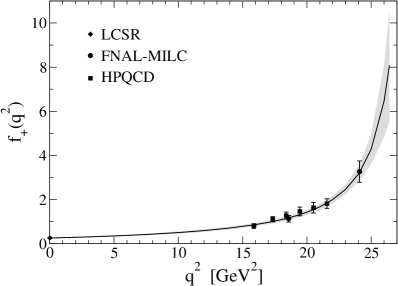
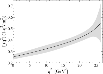
Figure 2: Left: the form factor $f_{+}(q^{2})$ given by Eqs. (38) and (39). The error band is given by the statistical uncertainties. As explained in the text, systematic errors coming from the parametrization are negligible in the semileptonic domain in our approach. The theoretical LCSR result from [12] and the lattice results from [13, 17] are also shown. Right: the numerator in (38) for the optimal parametrization.

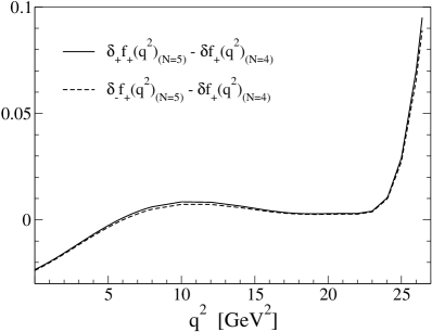
Figure 3: Change in the error with the number of parameters, $N$, in the physical region: the solid (dashed) line shows the difference between the $N=5$ and $N=4$ plus (minus) errors on the product $f_{+}(q^{2})(1-q^{2}/m^{2}_{B^{*}})$.

Table 3: Comparison of the form factor $f_{+}(q^{2})$ obtained at a variety of recoils in the lattice computations of FNAL-MILC [13, 16] (rows 1-3) and HPQCD [17] (rows 4-8), with the results of the combined fit in Eq. (39), to the parametrization given in Eq. (38). In the lattice results, the first error is the combined statistical and chiral extrapolation error, while the second is an 11% systematic for FNAL-MILC [13, 16] and a 9.5% error for HPQCD [17].

$q^{2}\,(\mbox{GeV}^{2})\hskip 28.45274pt$	$f_{+}(q^{2})_{\rm lattice}\hskip 85.35826pt$	$f_{+}(q^{2})_{\rm fit}$
15.87	0.799 $\pm$ 0.058 $\pm$ 0.088	$0.852\,^{+0.071}_{-0.070}$
18.58	1.128 $\pm$ 0.086 $\pm$ 0.124	$1.169\,^{+0.093}_{-0.092}$
24.09	3.263 $\pm$ 0.324 $\pm$ 0.359	$3.227\,^{+0.356}_{-0.352}$
17.34	1.101 $\pm$ 0.053 $\pm$ 0.105	$1.003\,^{+0.081}_{-0.080}$
18.39	1.273 $\pm$ 0.099 $\pm$ 0.121	$1.141\,^{+0.091}_{-0.090}$
19.45	1.458 $\pm$ 0.142 $\pm$ 0.139	$1.316\,^{+0.105}_{-0.104}$
20.51	1.627 $\pm$ 0.185 $\pm$ 0.155	$1.542\,^{+0.124}_{-0.123}$
21.56	1.816 $\pm$0.126 $\pm$ 0.173	$1.841\,^{+0.151}_{-0.149}$

The form factor calculated using the expression (38) and the parameters from Eq. (39) is shown in Fig. 2, where in the right panel we plot the $z$ polynomial in the numerator of Eq. (38). The error bands represent the purely statistical error. We emphasize that we do not use the linear approximation in the error propagation, but apply the standard $\Delta\chi^{2}$ analysis, i.e. by finding the range of variation of a given parameter corresponding to a change in $\chi^{2}$, minimized over all other parameters, by one unit. The unitarity constraint plays a nontrivial role, being responsible for the asymmetric errors, especially near the right end of the semileptonic range. For completeness, the values of the form factor are given in Table 2 for a sample of $q^{2}$ in the semileptonic domain. In Table 3 we compare the results of our combined fit with the lattice results used as input.

As seen from the values given in (VII), the gradual reduction of the systematic error with the increase of $N$ is balanced by the increase of the statistical error. It is of interest to compare the total error on the values of the form factor for $N=5$ and $N=4$. In Fig. 3 we plot the difference between these two errors as a function of $q^{2}$. For $N=5$ the error is purely statistical, for $N=4$ it is calculated by adding quadratically the statistical and the systematic errors, the later one obtained from (35). As we already noted, the error in the $N=5$ case is slightly not symmetric due to the unitarity constraint, therefore we present separately the difference between the “plus” and ”minus” $N=5$ errors and the $N=4$ one. Figure 3 shows that the difference between the errors is practically zero for most of the energy range, including the energies where lattice input is available. At low values of $q^{2}$, in particular at $q^{2}=0$, the total error decreases when passing from $N=4$ to $N=5$. On the other hand, at high values of $q^{2}$ the error for $N=5$ is larger than the $N=4$ error. One may ask whether it is not preferable to take as a best prediction the parametrization with $N=4$. In our opinion, this is not the case: the advantage of our prescription is that the systematic errors are negligible along the whole physical region. Thus, we avoid any bias related to the specific form of the truncation error for the determination of the form factor and of $V_{ub}$. Our results show that a representation of the form factor having a small uncertainty over the whole physical region, including its upper end, is not possible with the present input information.

From the above comment we expect even larger errors if the expression (38) is used to calculate the form factor outside the physical region. In particular, we consider the residue of $f_{+}(q^{2})$ at the pole $q^{2}=m_{B^{*}}^{2}$, defined as

$$r_{+}=\lim_{q^{2}\to m_{B^{*}}^{2}}(1-q^{2}/m_{B^{*}}^{2})\,f_{+}(q^{2}).$$ (41)

The systematic error, calculated using the prescription (35), is no longer negligible at the position $z_{*}=-0.504$ of the pole. From (38) and (39) we obtain

$$r_{+}=0.676\,\pm 0.608\,(stat)\pm 0.212\,(syst).$$ (42)

Alternatively, one can use a different conformal mapping, i.e. a different value of the parameter $t_{0}$ in (4), which allows a better accuracy in the high energy range. A reasonable choice is $t_{0}=t_{-}$, when the physical region $(0,\,t_{-})$ is mapped onto the interval (-0.518, 0) of the $z$ plane, and the pole position becomes $z(m_{B^{*}}^{2},t_{-})=-0.262$. Since the pole is closer to the origin, the systematic error at this point is now negligible already for the best fit with $N=4$ parameters, when we obtain

$$r_{+}=0.544\,\pm 0.165\,(stat)\pm 0.034\,(syst).$$ (43)

The value (42) can be converted to a prediction for $g_{B^{*}B\pi}=2r_{+}m_{B^{*}}/f_{B^{*}}$. Using, for instance, $f_{B^{*}}=0.196\pm 0.031\,{\rm GeV}$ [46], we obtain

$$g_{B^{*}B\pi}=37.\pm 33.\,(stat)\pm 12.\,(syst)\pm 6.(\delta f_{B^{*}}),$$ (44)

to be compared with the lattice result $g_{B^{*}B\pi}=47\pm 3\,{\rm(stat)}\pm 9\,{\rm(syst)}$ from [47]. The large statistical and systematic errors show that a reliable extraction of the residue from the extrapolation of our best fit is not possible. Additional information on the behavior of $f_{+}(q^{2})$ outside the physical region, like the absence of zeros, expected on general grounds for form factors [44], or the monotony, valid in some models [45], might improve the prediction. A more detailed study of this problem will be presented in a future work.

Before ending this section, let us make a few more comments on the standard analytic parametrization (3). We presented the results of fits to this parametrization in (32)-(VI) and in Fig. 1. As discussed in Sec. II, the parametrization (3) has a fake singularity at the unitarity threshold, $q^{2}=t_{+}$, which is expected to produce distortions in the behavior of the form factor at large values of $q^{2}$. For instance, from the fit with $N=5$ parameters, i.e. using four terms in the expansion (3) and the best values from (VI), we obtain

$$f_{+}(t_{-})=8.59\,^{+3.67}_{-3.55}\,(stat)\pm 1.89\,(syst),\quad[{\rm Eqs.(\ref{AGRS}),(\ref{N5t})}],$$ (45)

and the residue

$$r_{+}=0.956\,\pm 1.855\,(stat)\pm 2.140\,(syst),\quad[{\rm Eqs.(\ref{AGRS}),(\ref{N5t})}].$$ (46)

The larger systematic errors are explained in part by the fact that now the expansion has only four terms (unlike in (38), where an additional term was introduced using the threshold condition). The statistical errors are also larger than for the $N=5$ fit which uses our new parametrization, Eqs. (VII) and (42), showing that the singularity at threshold affects the behavior of the form factor near this point.

IX Determination of $|V_{ub}|$

As shown in Sec. VI, $|V_{ub}|$ is one of the parameters determined by our fit: the optimal value and the statistical error are given in Eq. (VI). We chose the parametrization such that the systematic error can be neglected along the whole physical region. Therefore, the determination of $|V_{ub}|$ will be free of systematic uncertainties. Adding an experimental error of $0.01\times 10^{-3}$ associated with the uncertainty in the $B^{0}$ lifetime [42], our final prediction is

$$|V_{ub}|=(3.54\pm 0.30)\times 10^{-3}.$$ (47)

This result depends of course on the theoretical and experimental input used, and will become more and more accurate as this input will improve. Our purpose in this work was mainly to prove the advantages of the simple parametrization Eq. (38) of the form factor, which we recommend as a useful tool in future data analyses.

The result (47) is consistent with the most recent prediction from exclusive $B\to\pi$ decays [4]. However, as discussed in Sec. II, the analysis in [4] is based on a parametrization that does not fully satisfy the constraints of analyticity and unitarity. Moreover, the statistical correlations in the lattice results are neglected there. Thus, our analysis puts the extraction of $|V_{ub}|$ from exclusive $B\to\pi$ decays on a more rigorous basis.

From the fit given in (VI) we obtain also

$$|V_{ub}|f_{+}(0)=(8.99\pm 0.72)\times 10^{-4}\,,$$ (48)

to be compared with the result $|V_{ub}|f_{+}(0)=(7.6\pm 1.9)\times 10^{-4}$ obtained with SCET and factorization [48].

X Conclusions

We proposed a simple analytic parametrization for the semileptonic $B\to\pi$ vector form factor $f_{+}(q^{2})$, by multiplying the factor accounting for the $B^{*}$ pole with a convergent expansion in powers of a conformal mapping variable. The parametrization has the correct behavior at the unitarity threshold and satisfies perturbative scaling and the constraint derived from the positivity of the correlation function of the $\bar{u}\gamma_{\mu}b$ current and its Hermitian conjugate. The latter was used also to define the systematic error due to the truncation of the expansion. By increasing up to $K=4$ the number of terms in the expansion, we obtained the representation given in Eqs. (38)-(39), where the systematic error can be neglected along the whole physical region. From the combined fit of our parametrization to experimental results for the differential decay rate and to theoretical results for the form factor, we obtained a prediction for $|V_{ub}|$ given in (47). Our result confirms that $|V_{ub}|$ extracted from the exclusive $B\to\pi$ decays is consistent with the global fits of the CKM matrix [49].

*

Appendix A

In this Appendix we show that unitarity allows one to derive a bound on the remainder of the expansion (11), defined as

$$\delta f_{+}(q^{2})=\frac{1}{1-q^{2}/m_{B^{*}}^{2}}\,\sum\limits_{K+1}^{\infty}b_{k}z^{k}\,.$$ (49)

For simplicity we omit the dependence of the coefficients and the variable $z$ upon $t_{0}$, which is kept fixed in the expressions given below.

Using (3) and (11) we express each coefficient $b_{k}$ as

$$b_{k}=\sum\limits_{j=0}^{k}\tilde{\eta}_{k-j}a_{j},\quad\quad k\geq 0\,,$$ (50)

where $\tilde{\eta}_{j}$ appear in the expansion

$$1/\Psi(z)=\sum\limits_{k=0}^{\infty}\tilde{\eta}_{j}z^{j}\,,$$ (51)

with $\Psi(z)$ given in Eq. (18). By the Cauchy inequality we obtain from (50)

$$|b_{k}|\leq\{\sum\limits_{j=0}^{k}\tilde{\eta}_{j}^{2}\,\sum\limits_{j=0}^{k}a_{j}^{2}\}^{1/2},\quad\quad k\geq 0\,,$$ (52)

and, using (7),

$$|b_{k}|\leq\{\sum\limits_{j=0}^{k}\tilde{\eta}_{j}^{2}\}^{1/2},\quad\quad k\geq 0\,.$$ (53)

Therefore, the remainder (49) is bounded in terms of calculable quantities

$$|\delta f_{+}(q^{2})|\leq\,\frac{1}{|1-q^{2}/m_{B^{*}}^{2}|}\sum\limits_{k=K+1}^{\infty}\{\sum\limits_{j=0}^{k}\tilde{\eta}_{j}^{2}\}^{1/2}\,|z|^{k}\,.$$ (54)

The upper bound (54) can be made sufficiently small for a certain $K$ and $|z|<1$. This follows from the properties of the coefficients $\tilde{\eta}_{j}$ defined in (51): indeed, the function $1/\Psi(z)$ has singularities on the boundary $|z|=1$, but it is analytic inside the disk $|z|<1$. Therefore, although the Taylor coefficients $\tilde{\eta}_{j}$ increase with $j$, the increase is such that sum $\sum_{k>K}\tilde{\eta}_{k}|z|^{k}$ can be made arbitrarily small for a certain $K$ and $|z|<1$. The same is true for the coefficients appearing in (54), this fact being obvious, in particular, if we use the upper bound $\{\sum\limits_{j=0}^{k}\tilde{\eta}_{j}^{2}\}^{1/2}<k\tilde{\eta}_{k}$, valid for sufficiently large $k$. Using this estimate, the sum in (54) is related to the remainder of the Taylor expansion of the derivative of the function $1/\Psi(z)$, which can be made arbitrarily small since the series is convergent for $|z|<1$.

References

- [1] M.C. Arnesen et al., Phys. Rev. Lett. 95, 071802 (2005).
- [2] J.M. Flynn and J. Nieves, Phys. Rev. D 75, 013008 (2007).
- [3] J.M. Flynn and J. Nieves, Phys. Lett. B 649, 269 (2007).
- [4] J.M. Flynn and J. Nieves, Phys. Rev. D 76, 031302 (2007).
- [5] S.B. Athar et al. (CLEO Collaboration), Phys. Rev. D 68, 072003 (2003).
- [6] N.E. Adam et al. (CLEO Collaboration), Phys. Rev. Lett. 99, 041802 (2007).
- [7] T. Hokuue et al. (Belle Collaboration), Phys. Lett. B 648, 139 (2007).
- [8] B. Aubert et al. (BABAR Collaboration) Phys. Rev. Lett. 97, 211801 (2006).
- [9] B. Aubert et al. (BABAR Collaboration) Phys. Rev. Lett. 98, 091801 (2007).
- [10] A. Khodjamirian et al., Phys. Lett. B 410, 275 (1997).
- [11] P. Ball and R. Zwicky, Phys. Rev. D 71, 014029 (2005).
- [12] G. Duplancic et al., J. High Energy Phys. 04 (2008) 014.
- [13] M. Okamoto et al., Nucl. Phys. Proc. Suppl. 140, 461 (2005).
- [14] M. Okamoto, Proc. Sci. LAT2005 (2006) 013, arXiv:hep-lat/0510113.
- [15] R.S. Van de Water and P.B. Mackenzie (Fermilab Lattice and MILC), Proc. Sci. LAT2006 (2006) 097.
- [16] P.B. Mackenzie et al. (Fermilab Lattice Collaboration, MILC Collaboration and HPQCD Collaboration), Proc. Sci. LAT2005 (2006) 207.
- [17] E. Dalgic et al., Phys. Rev. D 73, 074502 (2006).
- [18] J. Bailey et al., arXiv:0811.3640 [hep-lat].
- [19] L. Lellouch, Nucl. Phys. B479, 353 (1996).
- [20] G.P. Lepage and S.J. Brodsky, Phys. Rev. D 22, 2157 (1980).
- [21] R. Akhoury, G. Sterman and Y.P. Yao, Phys. Rev. D 50, 358 (1994).
- [22] P. Ball, Phys. Lett. B 644, 38 (2007).
- [23] D. Becirevic and A.B. Kaidalov, Phys. Lett. B 478, 417 (2000).
- [24] S. Okubo, Phys. Rev. D 4, 725 (1971).
- [25] S. Okubo, Phys. Rev. D 3, 2807 (1971).
- [26] C. Bourrely, B. Machet and E. de Rafael, Nucl. Phys. B189, 157 (1981).
- [27] I. Caprini, L. Lellouch and M. Neubert, Nucl. Phys. B530, 153 (1998).
- [28] C. Bourrely and I. Caprini, Nucl. Phys. B722, 149 (2005).
- [29] C.G. Boyd, B. Grinstein and R.F. Lebed, Phys. Lett. B 353, 306 (1995).
- [30] S.C. Generalis, J. Phys. G 16, 785 (1990).
- [31] C.G. Boyd, B. Grinstein and R.F. Lebed, Phys. Rev. Lett. 74, 4603 (1995).
- [32] C.G. Boyd, B. Grinstein and R.F. Lebed, Nucl. Phys. B461, 493 (1996).
- [33] T. Becher and R.J. Hill, Phys. Lett. B 633, 61 (2006).
- [34] R. Omnès, Nuovo Cim. 8, 316 (1958).
- [35] K.M. Watson, Phys. Rev. 95, 228 (1954).
- [36] S. Ciulli and J. Fischer, Nucl. Phys. 24, 465 (1961).
- [37] R.E. Cutkosky and B.B. Deo, Phys. Rev. 174, 1859 (1968).
- [38] C. Amsler et al. (Particle Data Group), Phys. Lett. B 667, 1 (2008).
- [39] K.G. Chetyrkin and A. Retey, Nucl. Phys. B583, 3 (2000).
- [40] M.A. Shifman, A.I. Vainshtein and V.I. Zakharov, Nucl. Phys. B147, 385, 448 (1979).
- [41] C. Bernard et al., Proc. Sci. LAT2007 (2007) 090, arXiv:0710.1118 [hep-lat].
- [42] E. Barberio et al. (Heavy Flavor Averaging Group (HFAG)), arXiv:0704.3575 [hep-ex].
- [43] D. Luenberger, Optimization by Vector Space Methods (Wiley, New York, 1969).
- [44] H. Leutwyler, arXiv:hep-ph/0212324.
- [45] N. Isgur and M.B. Wise, Phys. Rev. D 41, 151 (1990).
- [46] D. Becirevic and A. Le Yaouanc, J. High Energy Phys. 03 (1999) 021.
- [47] A. Abada et al., J. High Energy Phys. 02 (2004) 016.
- [48] C.W. Bauer et al., Phys. Rev. D 70, 054015 (2004).
- [49] J. Charles et al. (CKMfitter Group), Eur. Phys. J. C 41, 1 (2005).