Clustering of Luminous Red Galaxies III:
Detection of the Baryon Acoustic Peak in the 3-point Correlation Function

Abstract

We present the 3-point function $\xi_{3}$ and $Q_{3}=\xi_{3}/\xi_{2}^{2}$ for a spectroscopic sample of luminous red galaxies (LRG) from the Sloan Digital Sky Survey DR6 & DR7. We find a strong (S/N$>$6) detection of $Q_{3}$ on scales of 55-125 Mpc/h, with a well defined peak around 105 Mpc/h in all $\xi_{2}$, $\xi_{3}$ and $Q_{3}$, in excellent agreement with the predicted shape and location of the imprint of the baryon acoustic oscillations (BAO). We use very large simulations (from a cubic box of L=7680 Mpc/h) to asses and test the significance of our measurement. Models without the BAO peak are ruled out by the $Q_{3}$ data with 99% confidence. This detection demonstrates the non-linear growth of structure by gravitational instability between $z=1000$ and the present. Our measurements show the expected shape for $Q_{3}$ as a function of the triangular configuration. This provides a first direct measurement of the non-linear mode coupling coefficients of density and velocity fluctuations which, on these large scales, are independent of cosmic time, the amplitude of fluctuations or cosmological parameters. The location of the BAO peak in the data indicates $\Omega_{m}=0.28\pm 0.05$ and $\Omega_{B}=0.079\pm 0.025$ (for $h=0.70$) after marginalization over spectral index ($n_{s}=0.8-1.2$) linear $b_{1}$ and quadratic $c_{2}$ bias, which are found to be in the range: $b_{1}=1.7-2.2$ and $c_{2}=0.75-3.55$. The data allows a hierarchical contribution from primordial non-Gaussianities in the range $Q_{3}=0.55-3.35$. These constraints are independent and complementary to the ones that can be obtained using the 2-point function, which are presented in a separate paper. This is the first detection of the shape of $Q_{3}$ on BAO scales, but our errors are shot-noise dominated and the SDSS volume is still relatively small, so there is ample room for future improvement in this type of measurements.

I Introduction

The galaxy three-point function $\xi_{3}$ provides a crucial test and valuable statistical tool to investigate the origin of structure formation and the relationship between galaxies and dark matter (see Bernardeau et al. (2002) for a review). We will concentrate here on the reduced 3-point function $Q_{3}\simeq\xi_{3}/\xi_{2}^{2}$ defined in Eq.3 as the scaling expected from non-linear couplings (with $Q_{3}\simeq 1$). Measurements of the three-point function and other higher-order statistics in galaxy catalogs have a rich history (eg Peebles and Groth (1975), Fry and Peebles (1978), Baumgart and Fry (1991), Gaztanaga (1992), Bouchet et al. (1993), Fry and Gaztanaga (1994)). In the past decade, three-point statistics have confirmed the basic picture of gravitational instability from Gaussian initial conditions (Frieman and Gaztanaga (1994), Jing and Boerner (1998), Frieman and Gaztañaga (1999), Feldman et al. (2001)). The connection between these observables and theoretical predictions is best done on large scales, where the physics (gravity) is best understood, but the surveys previously available were not large enough to have good statistics on sufficiently large scales.

With the completion of large redshift surveys such as 2dFGRS (Colless et al. (2001)) and SDSS (York et al. (2000)) we expect measurement of higher-order statistics to provide tighter constraints on cosmology (Colombi et al. (1998), Szapudi et al. (1999), Matarrese et al. (1997), Scoccimarro et al. (2004), Sefusatti and Scoccimarro (2005)). First measurements of the redshift space $\xi_{3}$ in the 2dFGRS (Gaztañaga et al. (2005)) and SDSS (eg Nichol et al. (2006)) show good agreement with expectations (see also Kayo et al. (2004), Nishimichi et al. (2007), Kulkarni et al. (2007) and references therein).

We will assume here that the initial conditions are Gaussian. Current models of structure formation predict a small level of initial non-Gaussianities that we can neglect here. A popular parametrization of this effect is to assume that initial curvature perturbations, given by the gravitational potential, $\Phi$, are given by $\Phi=\Phi_{L}+f_{NL}~{}(\Phi_{L}^{2}-<\Phi_{L}^{2}>)$, where $\Phi_{L}$ is Gaussian and $f_{NL}$ is a non-linear coupling parameter of order unity. This produces non-Gaussianities in the matter density perturbations at wavenumber $k$ which, using the Poisson equation, are suppressed by the square of the horizon scale $k_{H}\equiv H_{0}/c$, so that: $Q_{3}\simeq 3f_{NL}(k_{H}/k)^{2}T(k)/D(a)$, where $T(k)\simeq 1$ is the so called CDM transfer function and $D(a)$ is the growth factor. In our analysis $(k_{H}/k)^{2}\simeq 10^{-3}$ so that these type of primordial non-Gaussianities produce negligible contribution to $Q_{3}$ for models with $f_{NL}\simeq 1$. A more detailed analysis of this will be presented elsewhere (see Sefusatti and Komatsu (2007) for a detailed forecast for this model). If the non-Gaussianities come from a non-linear coupling in the matter density field rather than in the gravitational potential, the resulting 3-point function will have a non-Gaussian contribution similar to that produced by non-linear bias $c_{2}$ (ie see Eq.13 below and Conclusions).

The shape and amplitude of $Q_{3}$ depends on galaxy bias, ie how galaxy light traces the dark matter (DM) distribution. This is both a problem and an opportunity. A problem because biasing can confuse our interpretation of the observations. An opportunity because one can try to measure the biasing parameters out of $Q_{3}$. This idea was first proposed by Fry and Gaztanaga (1993) and has been applied to the 3-point function and bispectrum of real data (Frieman and Gaztanaga (1994); Fry (1994); Feldman et al. (2001); Scoccimarro et al. (2001a); Verde et al. (2002); Gaztañaga et al. (2005); Nichol et al. (2006)).

This paper is the third on a series of papers on clustering of LRG. In the first two papers Cabré and Gaztañaga (2008a, b) we studied redshift space distortions on the 2-point correlation function. The reader is referred to these papers for more details on the LRG samples, simulations and the systematic effects. Similar LRG samples from SDSS have already been used by different groups to study the 2-point function (eg Eisenstein et al. (2005); Hütsi (2006); Percival et al. (2007); Padmanabhan et al. (2007); Blake et al. (2007)) and found good agreement with predictions in the BAO scales, where density fluctuations are at a level of few percent. This is encouraging and indicates that this sample is large and accurate enough to investigate clustering on such large scales.

In this paper we follow closely the methodology presented in 3 previous analysis. Barriga and Gaztañaga (2002) presented a comparison of the predictions for the two and three-point correlation functions of density fluctuations, $\xi_{2}$ and $\xi_{3}$, in gravitational perturbation theory (PT) against large Cold Dark Matter (CDM) simulations. Here we use the same method and codes to estimate the clustering in simulations. Gaztañaga and Scoccimarro (2005) extend these results into the non-linear regime and focus on the effects of redshift distortions and the extraction of galaxy bias parameters in galaxy surveys. Gaztañaga et al. (2005) apply this methodology to the 2dFGRS. Here we apply the very same techniques to the LRG data, so the reader is referred to these papers for more details.

Kulkarni et al. (2007) have also estimated $\xi_{3}$ using LRG galaxies from SDSS DR3, but focusing on smaller scales. We use DR6 which has 3 times the area (and volume) of DR3. We also use a volume limited sample and a different estimator for the correlation functions and errors, focusing on the largest scales.

II Theory

II.1 Definitions

The two and three-point correlation functions are defined, respectively, as

$$\mbox{$$}\xi_{2}(r_{12}) = \langle\delta(r_{1})\delta(r_{2})\rangle$$ (1)

$$\xi_{3}(r_{12},r_{23},r_{13}) = \langle\delta(r_{1})\delta(r_{2})\delta(r_{3})\rangle$$ (2)

where $\delta(r)=\rho(r)/\bar{\rho}-1$ is the local density fluctuation about the mean $\bar{\rho}=\langle\rho\rangle$, and the expectation value is taken over different realizations of the model or physical process. In practice, the expectation value is over different spatial regions in our Universe, which are assumed to be a fair sample of possible realizations (see Peebles 1980). A possible complication with this approach is the so call finite volume effects which result in potential estimation and ratio biases (eg see Hui and Gaztañaga (1999); Bernardeau et al. (2002)). For our samples we have checked using a large simulation that these potential estimation biases are small compared to the errors. This can be seen in Fig.2 below which shows a good agreement between predictions and mock simulations that have the same size than the SDSS sample that we used in our analysis. We use a simulation with about 512 more volume than the data. We split this large simulation into 512 subsamples and estimate the mean and error (from the variance) of the 2 and 3-point correlation functions in the 512 subsamples. We find that this mean agrees well, well within the error, with the corresponding correlation estimated in the full simulation. This indicates that the finite volume effects are negligible compared to errors (see also Fig.5 in paper IV, Gaztanaga et al. (2008)).

It is convenient to define a $Q_{3}$ parameter as Groth and Peebles (1977)

$$Q_{3} = \frac{\xi_{3}(r_{12},r_{23},r_{13})}{\xi_{3}^{H}(r_{12},r_{23},r_{13})}$$ (3)

$$\xi_{3}^{H} \equiv {\xi_{2}(r_{12})\xi_{2}(r_{23})+\xi_{2}(r_{12})\xi_{2}(r_{13})+\xi_{2}(r_{23})\xi_{2}(r_{13})},$$

where we have introduced a definition for the ”hierarchical” three-point function $\xi_{3}^{H}$. Note that, by homogeneity, the 3-point function $\xi_{3}$ or $Q_{3}$ can only depend on the distance between $r_{1}$, $r_{2}$ and $r_{3}$. This involves 3 variables that define the triangle formed by the 3 points. In principle $Q_{3}$ could depend on the geometry and scale of the triangle. Here we will use two of the triangle sides $r_{12}$, $r_{23}$ and $\mu$, the co-sinus of the angle between $\vec{r}_{12}$ and $\vec{r}_{23}$, which we call $\alpha$. Thus $Q_{3}=Q_{3}(r_{12},r_{13},\mu)$.

The $Q_{3}$ parameter was thought to be roughly constant as a function of triangle shape and scale (Peebles (1980)), a result that is usually referred to as the hierarchical scaling. Accurate measurements/predictions show that $Q_{3}$ is not quite constant in any regime of clustering, although the variations of $Q_{3}$ with scale and shape are small compared to the corresponding changes in $\xi_{2}$ or $\xi_{3}$, specially at small scales.

II.2 $Q_{3}$ and mode coupling

We will illustrate next how measurements of $Q_{3}$ provide a direct estimation of the non-linear mode coupling of density and velocity fluctuations. First consider the fully non-linear fluid equations that determine the gravitational evolution of density fluctuations, $\delta$, and the divergence of the velocity field, $\theta$, in an expanding universe for a pressureless irrotational fluid. In Fourier space (see Eq.37-38 in Bernardeau et al. (2002)):

$$\dot{\delta}+\theta=-\int dk_{1}dk_{1}\alpha(k_{1},k_{2})\theta(k_{1})\delta(k_{2})$$ (4)

$$\dot{\theta}+H\theta+{3\over{2}}\Omega_{m}H^{2}\delta=-\int dk_{1}dk_{1}\beta(k_{1},k_{2})\theta(k_{1})\theta(k_{2})$$

where derivatives are over time $d\tau=adt$ and $H=d\ln a/d\tau$. On the left hand side $\delta=\delta(k)$ and $\theta=\theta(k)$ are functions of the Fourier wave vector $k$. The integrals are over vectors $k_{1}$ and $k_{2}$ constrained to $k=k_{12}\equiv k_{2}-k_{1}$. The right hand side of the equation include the non-linear terms which are quadratic in the field and contain the mode coupling functions:

$$\alpha={k_{12}*k_{1}\over{k_{1}^{2}}}~{}~{}~{}~{};~{}~{}~{}~{}\beta={k_{12}^{2}(k_{2}*k_{1})\over{2k_{1}^{2}k_{2}^{2}}}$$ (5)

where “$*$” is the scalar product of the vectors (Eq.39 in Bernardeau et al. (2002)). This functions, $\alpha$ and $\beta$, account for the mixing of Fourier modes. Note that this functions are adimensional and depend on the geometry of the triangle formed by the two wave vectors $k_{1}$ and $k_{2}$ that contribute to $k=k_{2}-k_{1}$. The scalar product indicates that mode couplings are larger when the modes are aligned. Physically this means that density and velocity gradients created by (non-linear) gravitational growth will tend to be parallel.

Consider now the following perturbation expansions:

$$\delta=\sum_{i}~{}\delta_{i}~{}~{}~{}~{};~{}~{}~{}~{}\theta=\sum_{i}~{}\theta_{i}$$ (6)

The first terms, $\delta_{1}$ and $\theta_{1}$ in the above series are the linear solution of the fluid equations Eq.4, where we neglect the quadratic terms in the equations. The linear term yields $\dot{\delta}_{1}=-\theta_{1}$ for the first fluid equation in Eq.4. Combined with the second fluid equation yields the well known harmonic oscillator equation for the linear growth:

$$\ddot{\delta}_{1}+H\dot{\delta}_{1}-{3\over{2}}\Omega_{m}H^{2}\delta_{1}=0$$ (7)

This equation is valid in Fourier or in configuration space. In linear theory each Fourier mode evolves independently of the other and they all grow linearly out of the initial fields with the same growth function, ie $\delta_{1}=D(t)\delta_{0}$, where $\delta_{0}$ is the value of the field at some initial time and $D(t)$ is the linear growth function, which is a solution to the above harmonic equation. If the initial field $\delta_{0}$ is Gaussian then $\delta_{1}$ is also Gaussian. As shown above mode coupling is a non-linear effect. By construction, the next terms in the series of Eq.6, $\delta_{2}$ and $\theta_{2}$, are assumed to be quadratic in the linear terms, ie $\delta_{2}\propto\delta_{1}^{2}$. The solution for the second order can be found by just replacing the above expansion into the fluid equations keeping the second order terms in the equation. First order terms in the left side of the fluid equations in Eq.4 vanish by construction of the linear equation. We then find (see Eq.156 in Bernardeau et al. (2002)):

$$\delta_{2}(k) = \int dk_{1}dk_{2}F_{2}(k_{1},k_{2})\delta_{1}(k_{1})\delta_{1}(k_{2})$$ (8)

$$F_{2} = {5\over 7}\alpha+{2\over 7}\beta$$

Thus the second order term in the expansion is $\delta_{2}\propto F_{2}\delta_{1}^{2}$ and contains the mode coupling information through $F_{2}$.

Let’s consider now the observables, which are the 2 and 3-point correlation functions. Note that for an initially Gaussian field $\delta_{1}$ is also Gaussian so that $<\delta_{1}^{3}>=0$ and $<\delta_{1}^{4}>=3<\delta_{1}^{2}>^{2}$. At leading order the 2-point function $\xi_{2}$ is dominated by the linear evolution and the second to leading order term is zero because $<\delta_{1}\delta_{2}>=F_{2}<\delta_{1}^{3}>=0$. Thus we have $\xi_{2}(t)=D(t)^{2}\xi_{2}(0)$. The linear contribution to $\xi_{3}$ is also zero and the leading order in $\xi_{3}$ comes from having $\delta_{2}$ in one of the 3 points and $\delta_{1}$ in the other 2 points. For illustration, let us ignore for now the arguments of the 3 points, and see how things scale:

$$\xi_{3}=<\delta_{1}\delta_{1}\delta_{2}>\propto F_{2}<\delta_{1}^{4}>=3F_{2}<\delta_{1}^{2}>^{2}\propto F_{2}\xi_{2}^{2}$$ (9)

This is in agreement with the scaling $\xi_{3}=Q_{3}\xi_{2}^{2}$ in Eq.3. We therefore have that $Q_{3}$ at leading order is just proportional to $F_{2}$. This is exactly the case when we account for the arguments in the 3 points, as can be easily checked. The dependence of $F_{2}$ on the triangular configuration, ie through Eq.5, is all contained in the corresponding triangular configurations of $Q_{3}$, ie $Q_{3}=Q_{3}(r_{12},r_{13},\mu)$. This shows the interest of measuring $Q_{3}$: it provides a direct way to measure the mode coupling information in $F_{2}$, which includes the fully non-linear coupling in Eq.5. Higher order correlations just provide information about different combinations of coupling functions $\alpha$ and $\beta$.

II.3 Gravitational instability

We can now address the following question: is large scale structure produced by gravitational growth from small Gaussian fluctuations? We could answer this question by measuring $\xi_{2}(t)$. If we knew some initial conditions $\xi_{2}(0)$, we can then estimate $D(t)^{2}\simeq\xi_{2}(t)/\xi_{2}(0)$ and compare to the linear solution of Eq.7. By measuring $Q_{3}$ we can directly compare to $F_{2}$. This is independent of the linear test in $D(t)$ and does not require knowledge of the initial conditions $\xi_{2}(0)$. The result should in fact be independent of time.

We can also test gravitational growth with independence of time or initial conditions by using the linear relation between density and velocities, $\dot{\delta}_{1}=-\theta_{1}$. But this is a test of linear evolution and requires measurements of the velocity field (this, in fact, is tested using redshift space distortions in Paper-I of this series). $Q_{3}$ only needs density fields and explores the non-linear sector of gravity.

If the origin of structure is non gravitational (or gravity is non-standard) but the initial conditions are Gaussian, then on dimensional grounds we would also expect $\xi_{2}(t)=D(t)^{2}\xi_{2}(0)$ and $Q_{3}$ to be indepent of time. But both the amplitude and shape of $Q_{3}$ as a function of triangle configuration could be quite different if the fluid equations are different, either because of a non-standard cosmology or non-standard law of gravity (eg see Gaztañaga and Lobo (2001); Bernardeau et al. (2002)). In the standard case, the shape of $F_{2}$ is mostly independent of cosmological parameters (eg $\Omega_{m}$, $\Omega_{\Lambda}$ or $\Omega_{b}$), time or the amplitude of fluctuations Bernardeau et al. (2002). As shown above, density and velocity gradients produced by non-linear evolution are parallel which results in enhancement of clustering for elongated triangles. The exact amplitude as a function of triangular shape provides a finger print for non-linear gravitational growth. It is purely a non-linear effect that is not present in the initial conditions (which are assumed to be Gaussian with $Q_{3}=0$). Unfortunately, the prediction for $Q_{3}$ depends not only on the mode coupling $F_{2}$ but also on the slope of the initial $\xi_{2}(0)$. Models with relatively more large scale power (ie smaller slope) produce structures with larger coherence which give rise to more anisotropic structures and stronger shape dependence in $Q_{3}$. Fortunately the shape of $\xi_{2}$ can also be estimated from data and one can then test the mode coupling predictions for $F_{2}$, as we will show below.

II.4 Shape dependence and BAO

As mentioned above, there is a degeneracy in the shape of $Q_{3}$ between dark matter density $\Omega_{m}$ and baryon density $\Omega_{B}$ because they produce degenerate slopes in $\xi_{2}$. This degeneracy is broken by the presence of the BAO peak, but this requires a measurement at 100 Mpc/h scales. To illustrate this, consider a power law spectrum $P(k)=Ak^{n}$. In this case (see  Bernardeau et al. (2002) and references therein):

$$\xi_{3}(r_{12},r_{23},\mu)=\left[\frac{10}{7}+\frac{n+3}{n}\mu(\frac{r_{12}}{r_{23}}+\frac{r_{23}}{r_{12}})+\right.$$

$$\left.+\frac{4}{7}\frac{(3-2(n+3)+(n+3)^{2}\mu^{2})}{n^{2}}\right]\xi_{2}(r_{12})\xi(r_{23})+\cal{P}$$

where $\cal{P}$ stands for permutations of the indexes 123, and $\mu$ is the co-sinus of the angle between $\vec{r}_{12}$ and $\vec{r}_{23}$, which we call $\alpha$. Here we will only show results as a function of $\alpha$ for fixed $r_{12}$ and $r_{23}$. The above formula is only valid for a power-law spectrum. For CDM we will use a full calculation as explained below.

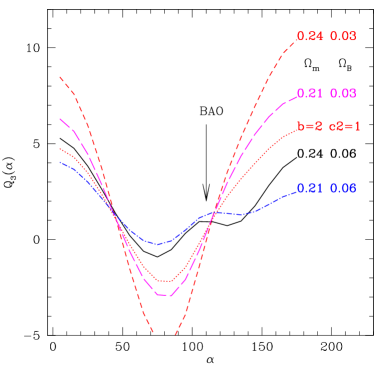
Elongated or “collapsed configurations” are those with $\alpha\simeq 0$ or $\alpha\simeq 180$ deg. We use the term ”strong configuration dependence” when there is a significant difference between the collapsed and the perpendicular configurations. By ”weak configuration dependence” we mean that $Q_{3}$ is “hierarchical” (ie constant as a function of $\alpha$). $Q_{3}(\alpha)$ flattens with the decrease of the spectral index $n$ and for larger $n$ has a strong configuration dependence with a characteristic “V” shape. This corresponds to a larger probability of finding 3 points aligned, a direct consequence of gravitational infall that enhances the filaments that are characteristic of large scale structure both in simulations and real data. In a CDM spectrum this dependence on $n$ translates into flat $Q_{3}$ (rounder structures) at small scales progressively getting stronger V-shape as the effective $n$ gets larger because of the CDM transfer function. At a fixed scale, the V-shape gets more pronounced when we increase $\Omega_{m}$ or when we decrease $\Omega_{B}$. This is just due to the effect of $\Omega_{m}$ and $\Omega_{B}$ in the CDM transfer function, which changes the effective spectral index $n$. If we fix the shape of the $P(k)$ spectrum, the values of $\Omega_{m}$ and $\Omega_{B}$ have very little effect on $Q_{3}$, as mentioned above.

These points are illustrated in Fig.1 which shows perturbation theory predictions for $Q_{3}$. For this calculation we use Eq.(8) in Barriga and Gaztañaga (2002), where different scales and triangular configurations are also shown. Here we focus on the results of $Q_{3}$ around the BAO scales. For high values of $\Omega_{B}$ a baryonic peak emerges in $Q_{3}$ and this peak could be used as a cosmological prove or to break the $\Omega_{m}-\Omega_{B}$ degeneracy. The peak is present in all $\xi_{2}$, $\xi_{3}$ and $Q_{3}$. As far as we know this is the first calculation illustrating how the BAO peak shows in $Q_{3}(\alpha)$.

Figure 1: Perturbation theory predictions for the reduced 3-point function $Q_{3}$ for different values of $\Omega_{m}$ and $\Omega_{B}$, as labeled in the Figure. All cases are unbiased, except for dotted line which corresponds to $\Omega_{m}=0.24$ and $\Omega_{b}=0.03$ with $b_{1}=2$ and $c_{2}=1$. This is for triangles with two sides fixed to $r_{12}=33\pm 5$ Mpc/h and $r_{13}=88\pm 5$ Mpc/h as a function of the interior angle $\alpha$ between this two sides. As $\alpha$ varies from $0-180$ degrees the third side of the triangle changes from $r_{23}=55$ Mpc/h to $r_{23}=121$ Mpc/h. For high values of $\Omega_{B}$ a BAO peak (marked by the arrow) shows at $\alpha=115$ degrees, which corresponds to $r_{23}=106$ Mpc/h. The precise location depends on the cosmology used.

Predictions in redshift space are harder to make (see Gaztañaga and Scoccimarro (2005)), but on large scales simulations show that redshift distortions in $\xi_{3}$ and $\xi_{2}^{2}$ cancel out in $Q_{3}$, and we do not expect deviations from PT tree-level predictions (see Fig.2 below).

II.5 Biasing

The value and shape of $Q_{3}(\alpha)$ changes with galaxy bias. On very large scales we expect that galaxy fluctuations $\delta_{G}$ can be modeled as a local (but non-linear) function of the corresponding matter fluctuations $\delta$, so that $\delta_{G}\simeq F[\delta]$. For small fluctuations, $\delta\ll 1$, we can expand this local function as:

$$\delta_{G}\simeq F[\delta]\simeq\sum_{i}~{}{b_{i}\over{i!}}~{}\delta^{i},$$ (11)

where $i=0$ comes from the requirement that $\langle\delta_{G}\rangle=0$. It then follows (see Fry and Gaztanaga (1993), Frieman and Gaztanaga (1994)) that:

$$\xi_{2}^{G}(r) \simeq b_{1}^{2}~{}\xi_{2}(r)$$ (12)

$$Q_{3}^{G} \simeq {1\over{b_{1}}}~{}\left(Q_{3}+c_{2}\right)$$ (13)

where $c_{2}\equiv b_{2}/b_{1}$, and the $\simeq$ sign indicates that this is the leading order contribution in the expansion given by Eq. (11) above. Thus, in general, the linear bias prescription is not accurate for higher-order moments even when $\delta\ll 1$, the reason being that non-linearities generate non-Gaussianities of the same order as those of gravitational origin. The linear bias term $b_{1}$ can produce distortions in the shape of $Q_{3}$, while the non-linear terms $c_{2}$ only shifts the curve. This is illustrated by the dotted line in Fig.1. It is therefore possible, but challenging, to use the shape of $Q_{3}^{G}$ in observations, when compared to the DM predictions, to separate $b_{1}$ from $c_{2}$ in the above relation. This gives an estimate of the linear bias $b_{1}$ which is independent of the overall amplitude of clustering (eg. $\sigma_{8}$). This approach has already been implemented for the skewness $S_{3}$ Gaztanaga (1994); Gaztanaga and Frieman (1994), the bispectrum Frieman and Gaztanaga (1994); Fry (1994); Feldman et al. (2001); Verde et al. (2002) or the angular 3-point function Frieman and Gaztañaga (1999) and has been used to forecast future analysis Sefusatti et al. (2006).

Figure 2: Measurements of $Q_{3}$ as in Fig.1 in dark matter (left panel) and groups (right panel) from the MICE7680 mock simulations. Mean and errors are estimated from 512 subsamples of $~{}1(Gpc/h)^{3}$. This is compared to the PT predictions in real space (dashed line) and corresponding biasing predictions for groups (continuous lines) Triangles and squares correspond to measurements in real and redshift space respectively. Two dotted lines shows the result for two single $1(Gpc/h)^{3}$ realizations (#20 and #21), in redshift space.

III Simulation and errors

To check our codes and estimate errorbars, we have used a comoving output at z=0 of a MICE simulation, run in the super computer Mare Nostrum in Barcelona by MICE consortium (www.ice.cat/mice). The simulation contains $2048^{3}$ dark matter particles, in a cube of side 7680Mpc/h (which we call MICE7680), $\Omega_{M}=0.25$, $\Omega_{b}=0.044$, $\sigma_{8}=0.8$, $n_{s}=0.95$ and $h=0.7$. This simulation uses the power spectrum of Eisenstein and Hu (1998) (EH from now on). To be consistent, the same approximation has also been used for the predictions. We assume here that this EH fit is good enough approximation for the precision in our analysis, but we note that Sanchez et al. (2008) found that on the BAO scale this approximation is only accurate at the few percent level. We also use the EH fit with “no wiggles” which for each cosmological model produces a match to the smoothed shape of the power spectrum without the BAO wiggles. This is equivalent to the removal of the BAO peak in the correlation function but keeping the same correlation as a based line. Note that we have chosen to displayed our results in terms of $\Omega_{m}$ and $\Omega_{B}$ for a fixed $h=0.7$.

The observed LRG galaxies are at a mean cosmic time of $z=0.3$ rather than cosmic time $z=0$ in our simulations. In principle, this should result in a slightly larger amplitude for the clustering in the simulations, because it corresponds to a later cosmic time. But the simulations have a lower normalization, $\sigma_{8}=0.80$, than the value of $\sigma_{8}=0.85$ inferred for the LRG galaxies after accounting for the effect of bias (see Paper I). This two effects partially compensate each other and the net result is that simulations have very similar clustering amplitude to that inferred in the LRG data.

To simulate biasing we select groups of particles using friend-of-friends with linking scale of $0.20$. We find a total of 107 million groups with more than 5 particles ($M>1.87\times 10^{13}$). These groups approximately correspond to DM halos when the number of particles in the group is larger than few tens of particles Evrard et al. (2008). When the number of particles is smaller than this, the group might not always correspond a virialized DM halo. But in any case, these groups sample high density regions which are biased tracers of the dark matter distribution. We can produce different mock galaxy catalogs by choosing the group richness (ie mass or number of particles). Very massive groups are more biased and more rare than smaller groups. What we do here is to select the group mass cut-off to reproduce the galaxy clustering in the LRG observations. It turns out that when we do this we get a number density of groups which is quite similar to the number density of LRG galaxies. Our mock catalogs are not realistic in the sense that we have not simulated the physics of galaxy formation. But we only use these catalogs for error estimation. Errors depend on the statistical properties of the simulation and not on process that produce such statistics. For our purposes here, all we need from mock simulations is that they have approximately the same volume, bias $b$, number density and similar values of $\xi_{2}$ and $\xi_{3}$ that observations. Errors only depend on this quantities.

We have also used a MICE simulation with $2048^{3}$ dark matter particles, in a cube of side 3072Mpc/h (which we call MICE3072, same parameters as MICE7680) which has 15 times better mass resolution to check for mass resolution effects. We find very similar results in both cases, but obviously MICE7680 provides more sampling volume to estimate reliable errors.

When we select groups with $M>2-4\times 10^{13}$, both the clustering amplitude ($b_{1}\simeq 1.9-2.2$ for $\sigma_{8}=0.8$) and the number density ($\bar{n}\simeq 4-6\times 10^{-5}$) are similar to the real LRG galaxies in our SDSS sample (the range reflects the fact that the actual number depend on LRG sample used). As the mock simulations are similar to the real data we will use the variance of clustering in the simulations to estimate errorbars for our analysis. The resulting errors from simulations are typically in good agreement with JK errors from the real data (see paper I for details). We will also check if we can recover the theory predictions for $Q_{3}$ by using mock simulations with similar size as the real data.

We have divided the big MICE7680 cube in $8^{3}$ sub-cubes, each of side 961Mpc/h and apply the LRG SDSS mask to obtain $N_{M}=512$ LRG mocks from both dark matter and groups. From the $N_{M}$ mock catalogs, we can estimate what we call the Monte Carlo (MC) covariance matrix:

$$C_{ij}=\frac{1}{N_{m}}\sum_{k=1}^{N_{m}}(\xi(i)^{k}-\widehat{\xi}(i))(\xi(j)^{k}-\widehat{\xi}(j))$$ (14)

where $\xi(i)^{k}$ is the measure of $\xi_{2}$, $\xi_{3}$ or $Q_{3}$ in the k-th mock simulation ($k=1,...N_{m}$) and $\widehat{\xi}(i)$ is the mean over $N_{m}$ realizations. The case i=j gives the diagonal error (variance).

Figure 3: Here we show the first 6 eigenvectors in the SVD using 512 subsamples in MICEL7680. Bottom panel shows the first 3 principal components (dashed, continuous and long-dashed lines) and the top panel shows the next 3 components, ranked by amplitude. While the $\Omega_{m}-\Omega_{B}$ constraints are degenerate using the first 3 components, this degeneracy is broken by using more eigenvectors because they can separate BAO features.

Figure 4: Contours of constant $\Delta\chi^{2}=1,2.3,4,6.2.$ and $9$ obtained from fitting models to measurements in dark matter (left panel) and groups (right panel) in MICE7680 mock simulations using SVD with MC covariance matrix corresponding to a Survey of about 1 $Gpc^{3}/h^{3}$. The crossing lines show the input values in the simulations, while the cross shows the best fit value. At 1-sigma, best fit is in excellent agreement with the input. But at 2-sigma there is a secondary peak and a strong degeneracy in the $\Omega_{B}-\Omega_{m}$ plane.

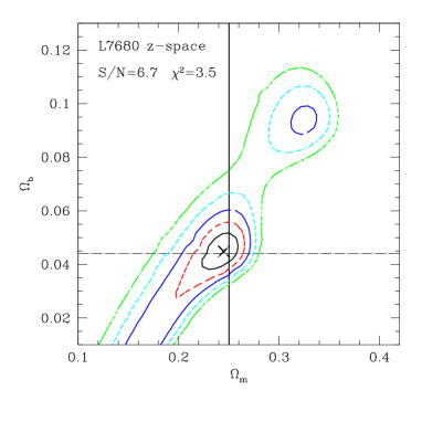
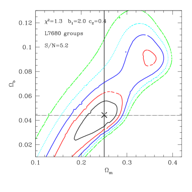
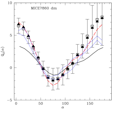
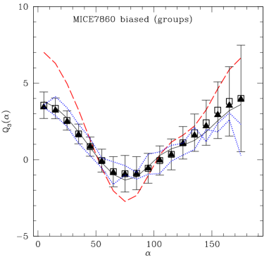
Fig.2 compares the mean and errors in the MICE7680 mocks with the PT predictions (dashed lines) in real space. At these large scales, results in real space are almost identical to redshift space for both dark matter (left panel) and groups with $M>1.87\times 10^{13}$ (right panel). The PT predictions and the biasing predictions work remarkably well. For bias we have used $b_{1}=1.9$ and $c_{2}=0.2$ (continuous lines). The value $b_{1}=1.9$ is estimated empirically from the ratio of the 2-point function of the groups to that of dark matter. This ratio is fairly constant for $r>11Mpc/h$. The non-linear bias $c_{2}$ produces a global shift that we have just fitted to the data. These estimated values of $b_{1}$ and $c_{2}$ agree very well with halo model prediction Scoccimarro et al. (2001b) for the mass of these groups. We note that we show the mean of the 512 mocks with errors from the dispersion in redshift space, which are slightly smaller (10-30%) than in real space. Dotted lines show results from two of the 512 realizations, illustrating the strong covariance in $Q_{3}(\alpha)$.

We apply a $\chi^{2}$ method to fit the models by inverting the covariance matrix $C_{ij}$, as explained in Gaztañaga and Scoccimarro (2005). Before inverting $C_{ij}$ in Eq.(8), notice that the values of $C_{ij}$ are estimated in practice to within a limited resolution in Eq.14, $\Delta C_{ij}\simeq\sqrt{2\over{N_{m}}}$. Therefore if the number of mocks $N_{m}$ is small or if there are degeneracies in $C_{ij}$, the inversion will be affected by numerical instabilities. In order to eliminate this problem, we perform a Singular Value Decomposition (SVD) of the matrix. By doing the SVD decomposition, we can choose the number of modes we wish to include in our $\chi^{2}$ by effectively setting the corresponding inverses of the small singular values to zero. In practice, we work only with the subspace of “dominant modes” which satisfy $\lambda_{i}^{2}>\sqrt{2/N_{m}}$ which is the resolution to which we can estimate the covariance matrix elements. Typically results converge after using a few singular values. Most of the times there is no gain in using more components which indicates that the effective number of degrees of freedom is smaller than the number of bins. Sometimes the fit gets bad when using larger number of components, which indicates instabilities in the covariance inversion. The results presented here are quite robust. We find that they are basically the same when we use different covariance matrices, corresponding to samples with different amplitude of clustering or different shot-noise, within the range that roughly matches the data. In particular, results are quite similar when we use DM particles mocks instead of groups mocks to estimate $C_{ij}$. The absolute errors in $Q_{3}$ are roughly the same for dark matter and groups, despite the difference in the amplitude. This give us confidence that what we find in real data is not an artifact of our analysis.

Fig.3 shows the first 6 eigenvectors or principal components, which resemble an harmonic decomposition of $Q_{3}(\alpha)$, as proposed by Szapudi (2004). The first component is roughly a constant, like a monopole, the second component corresponds to the ”V” shape mentioned above, like a quadrupole, and the third (short-dashed line) is similar to a dipole. The next components resemble higher multipoles and can be combined to define localized structure in $Q_{3}(\alpha)$. With the first two components it is not possible to break the $\Omega_{B}-\Omega_{m}$ degeneracy, given the errorbars. We have checked this in both the LRG data and the simulations. As we increase the number of multipoles we can see how the degeneracy in the $\Omega_{B}-\Omega_{m}$ plane begins to break down. The BAO feature only shows in the higher components and breaks the $\Omega_{B}-\Omega_{m}$ degeneracy for large values of $\Omega_{B}>0.03$. Lower values show no significant BAO peak, given the errors, and this results in a strong degeneracy in $\Omega_{B}-\Omega_{m}$ . We have played with the models and find that even if we artificially reduce the errors we need more that 2 eigenvalues to have a $\Omega_{B}$ detection.

In Fig.4 we show how well we can recover the values of $\Omega_{m}-\Omega_{b}$ from the mocks shown in Fig.2. We use 9 singular values, as in the LRG data, but results are quite similar from 5 to 9 singular values. In the case of dark matter (left panel in Fig.4), we do not include biasing parameters. In the case of groups (right panel) the results are marginalized for $b_{1}=1.7-2.2$ and $c_{2}=0.0-5.0$ . The best fit value is in excellent agreement with the input values both for $\Omega_{m}-\Omega_{b}$ and for $b_{1}-c_{2}$. This illustrates that fitting $b_{1}$ and $c_{2}$ from $Q_{3}$ in groups could be used to roughly estimate the mass of the groups or galaxy clusters. But even when we recover well the input value, note how errors are large and produce degenerate values at 2-sigma level for the size of our mock sample. As we will see below, this is because $\Omega_{b}$ is low in the simulation. The volume of data in a single mock, of about 1 (Gpc/h)³, is not large enough to break the $\Omega_{m}-\Omega_{b}$ degeneracy for low values of $\Omega_{b}$. This could be improved by using more shape configurations in $Q_{3}$ or smaller smoothing scales (we use cubic pixels with 11 Mpc/h on a side). The second (weaker) minimum $\chi^{2}$ that shows in Fig.4 for larger values of $\Omega_{b}\simeq 0.09$ corresponds the case where the BAO peak moves to smaller values of $\alpha$ and overlaps with the valley of the ”V” shape in $Q_{3}(\alpha)$. The $Q_{3}$ amplitude is low and the relative error is large in this region. This allows a BAO peak to be compatible with the simulations. This will also affect our LRG measurements in observations, although in this case the relative error is much smaller thanks to the non-linear bias $c_{2}$ which increases the overall amplitude of $Q_{3}(\alpha)$ and allows a more significant detection of $\Omega_{b}$.

IV Data and Analysis

IV.1 Data Sample

The luminous red galaxies (LRGs) are selected by color and magnitude to obtain intrinsically red galaxies in Sloan Digital Sky Survey (SDSS). See Eisenstein et al. (2001) or http://www.sdss.org for a complete description of the color cuts. These galaxies trace a big volume, around $1Gpc^{3}h^{-3}$, which make them perfect to study large scale clustering. LRGs are red old elliptical galaxies, which are usually passive galaxies, with relatively low star formation rate. Since they reside in the centers of big halos they are highly bias with $b\simeq 2$, between regular galaxies and clusters.

LRG’s are targeted in the photometric catalog, via cuts in the (g-r, r-i, r) color-color-magnitude cube. Note that all colors are measured using model magnitudes, and all quantities are corrected for Galactic extinction following Schlegel et al. (1998). The galaxy model colors are rotated first to a basis that is aligned with the galaxy locus in the (g-r, r-i) plane according to:

$c_{\perp}$= (r-i) - (g-r)/4 - 0.18

$c_{||}$= 0.7(g-r) + 1.2[(r-i) - 0.18]

Because the 4000 Angstrom break moves from the g band to the r band at a redshift z $\simeq$ 0.4, two separate sets of selection criteria are needed to target LRGs below and above that redshift:

Cut I for z $<$ 0.4

rPetro $<$ 13.1 + $c_{||}$ / 0.3

rPetro $<$ 19.2

$|c_{\perp}|$ $<$ 0.2

$mu_{50}$ $<$ 24.2 mag $arcsec^{-2}$

$r_{PSF}$ - $r_{model}$ $>$ 0.3

Cut II for z $>$ 0.4

$r_{Petro}$ $<$ 19.5

$|c_{\perp}|$ $>$ 0.45 - (g-r)/6

g-r $>$ 1.30 + 0.25(r-i)

$mu_{50}$ $<$ 24.2 mag $arcsec^{-2}$

$r_{PSF}$ - $r_{model}$ $>$ 0.5

Cut I selection results in an approximately volume-limited LRG sample to z=0.38, with additional galaxies to z $\simeq$ 0.45. Cut II selection adds yet more luminous red galaxies to z $\simeq$ 0.55. The two cuts together result in about 12 LRG targets per $deg^{2}$ that are not already in the main galaxy sample (about 10 in Cut I, 2 in Cut II). The radial distribution and magnitude-redshift diagrams for these galaxies are shown in Paper I Cabré and Gaztañaga (2008a).

We k-correct the r magnitude using the Blanton program ’kcorrect’ . We need to k-correct the magnitudes in order to obtain the absolute magnitudes and eliminate the brightest and dimmest galaxies. We have seen that the previous cuts limit the intrinsic luminosity to a range $-23.2<M_{r}<-21.2$, and we only eliminate from the catalog some few galaxies that lay out of the limits. Once we have eliminated these extreme galaxies, we still do not have a volume limited sample at high redshift. For the 2-point function analysis we account for this using a random catalog with identical selection function but 20 times denser (to avoid shot-noise) . The same is done in simulations. Computationally this is very time consuming (specially as there are 512 simulations) because it involves $N^{2}$ operations where $N\simeq 10^{6}$. For the 3-point, using the random catalogs would involve $N^{3}$ operations which begins to be very challenging with current computer power. We will therefore use a different estimator based on a pixelization of the sample. This estimator is ideally match to a volume limited sample, where the full volume is equally sampled and there is no radial selection function (we still have angular mask and radial boundaries).

For the 3-point function analysis presented in the paper we select a volume limited sample with $-22.5<M_{r}<-21.5$ and $z=0.15-0.38$ from the spectroscopic sample of LRG in the SDSS DR6. We choose this particular sample because it is the best compromise between volume and number density. There are about $40,000$ LRG galaxies in this sample ($\bar{n}\simeq 4\times 10^{-5}$).

IV.2 Correlation functions

We estimate the correlation functions with a fast algorithm described in some detail in Barriga and Gaztañaga (2002); Gaztañaga et al. (2005). This algorithm allows a fast calculation of two and three-point function for millions of points. The first step is to discretize the simulation box into $Lsize^{3}$ cubic cells. We assign each particle to a node of this new latticed box using the nearest grid point particle assignment. We precalculate the list of relative neighbors to any given node in the lattice. To compute now the two-point and three-point correlation functions we use:

$$\mbox{$$}\xi_{2}(r_{12}) = {\sum_{i,j}\delta_{i}\delta_{j}\over{\sum_{i,j}1}}$$ (15)

$$\xi_{3}(r_{12},r_{23},r_{13}) = {\sum_{i,j,k}\delta_{i}\delta_{j}\delta_{k}\over{\sum_{i,j,k}1}}$$ (16)

where $i$ extends over all nodes in the lattice, $j$ over the list of precalculated neighbors that are at a distance $r_{12}\pm dr/2$ from $i$, and $k$ is over the neighbors at distance $r_{23}\pm dr/2$ from $j$ and $r_{13}\pm dr/2$ from $i$. We take $dr$ to be equal to the pixel size.

There are two sources of errors in this estimation: a) Shot-noise which scales as one over the square root of the number of pairs or triplets in each bin b) sampling variance which scales with the amplitude of the correlations. It is easy to check that for the size and density of our sample the shot-noise term dominates over the sampling variance error. This has been checked in detailed by using DM simulations which have a large density and can be diluted to explore the shot-noise contribution to the error budget (see also Paper I).

We choose cubical pixels of $dr=11$ Mpc/h on the side. This is an adequate compromise to measure BAO. We want this number to be as large as possible to reduce shot-noise and to average over many triangles in a fast way. On the other hand, we need a good resolution to avoid loosing too much shape and BAO information. Once the pixel size is fixed to $dr=11$ Mpc/h we are forced to use $r_{12}>3dr$ which is the smaller distance that does not distort the $Q_{3}$ shape Barriga and Gaztañaga (2002). To reach the BAO scale we need $r_{13}>8dr$. So this fixes our choice of triangles. The 2-point function for this sample and pixelization is shown in Fig.B11 of Paper I Cabré and Gaztañaga (2008a).

IV.3 Results

After the release of DR6, Swanson et al. (2008) provided mask information in a readily usable form, translating the original mask files extracted from the NYU Value-Added Galaxy Catalog (Blanton et al., 2005), from MANGLE into Healpix format (Górski et al., 2005). Cabré and Gaztañaga (2008a) describe how they constructed a survey ”mask” for LRGs and tested the impact of the mask on clustering measurements using mock catalogs. Using the same techniques, we have also examined the correlation function of LRGs in DR7, which has become available since the submission of Cabré and Gaztañaga (2008a). In Fig. 5 we plot a summary of the possible systematics in the estimation of the $Q_{3}$ measurements. Our main result, that will be used for comparison with models, is shown as a shaded region, corresponding to the 1-sigma region. Results using different masks or the DR7 release are quite similar despite variations of $\sim 17\%$ in the fraction of galaxies or area used in the different cuts. We also show comparison to the results using all galaxies (open squares), rather than just a volume limited subsample. In this case we define density fluctuations using the local mean density provided by the random catalogs, rather than the overall mean density as we do for volume limited catalogs. The result is noiser (because of the shot-noise in the random catalogs) but in very good agreement with the other measurements. Evolutionary effects (that change the mean density) or magnitude effects do not seem important in this sample. We conclude that the results are very robust to the systematic variations that we have tried, and choose to use our default DR6 volume limited sample because this is the one that have been more tested and is the bases for our error analysis.

Figure 5: Estimations of $Q_{3}$ as in Fig.1 from observations using different samples and masks. Closed (red) squares and (red) shaded region show the main measurements and errors used in this paper, ie for a volume limited sample from DR6 with a magnitude range $-22.5<M<-21.5$ and $0.15<z<0.38$. Closed (blue) circles show the corresponding result in the DR7 sample. Open and closed triangles show the DR6 results using the MANGLE mask of Swanson et al. (2008) with greater than 0.0 or 0.8 completeness fractions. Open squares use all magnitudes. The (black) continuous line correspond to our best fit model in Fig.6

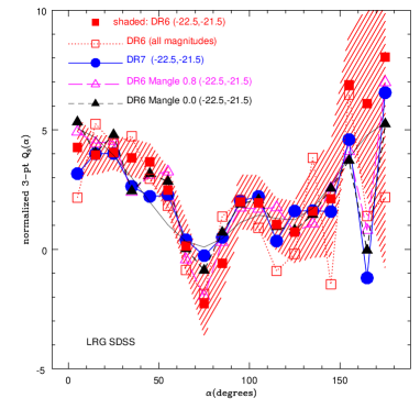
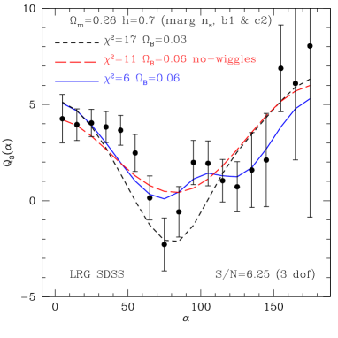
Fig.6 shows a comparison of $Q_{3}(\alpha)$ measurements in the LRG sample with models. There is a good resemblance with what is expected from theory, ie compared to Fig.1, with a peak at $\alpha\simeq 100$ deg. which resembles much the BAO peak predicted by models. As our signal is shot-noise dominated one may wonder if this peak could be produce by noise fluctuations.

Figure 6: Values of $Q_{3}$ as Fig.1, this time comparing three of the biased models (lines) to observations in LRG galaxies (symbols with errorbars). The total signal-to-noise in this detection is 6.25. Models have $\Omega_{m}=0.26$ and $h=0.7$. with $\Omega_{b}=0.03$ (short-dashed lines) or $\Omega_{b}=0.06$ (continuous line). Long-dashed uses EH fit with the no-wiggles (ie no BAO peak, but otherwise equal baseline spectrum) while the other lines includes the BAO peak in the models. We have marginalized over biasing parameters and spectral index and show the best fit in each case. The high $\Omega_{b}=0.06$ model has a minimum $\chi^{2}=6$ (with 3 degrees of freedom) which is significantly smaller than the mini-mun $\chi^{2}=17$ for the $\Omega_{b}=0.03$ model. The BAO peak shows at $\alpha=100$ in both the model with $\Omega_{b}=0.06$ and the data. The best fit model without BAO peak has $\chi^{2}>11$, ie a probability smaller than 1% of being correct.

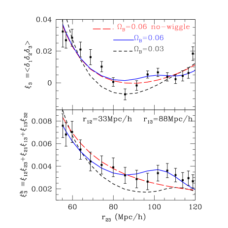
An indication that this signal is real comes from Fig.7. Detection of the BAO peak using the hierarchical product $\xi_{3}^{H}$ of 2-point function, as shown in Fig.7, is in excellent agreement with previous detections Eisenstein et al. (2005) and results over the very same sample in Paper I of this series Cabré and Gaztañaga (2008a). The peak seems to be detected in all $\xi_{3}$, $Q_{3}$ and $\xi_{2}$ and products.

Figure 7: Separate measurements of $\xi_{3}$ (top panel) and hierarchical $\xi_{3}\equiv\xi_{2}(r_{12})\xi_{2}(r_{23})+\xi_{2}(r_{21})\xi_{2}(r_{13})++\xi_{2}(r_{13})\xi_{2}(r_{32})$ (bottom panel). The models are as in Fig.6, ie $\Omega_{b}=0.03$ (short-dashed line) and $\Omega_{b}=0.06$ with (continuous line) and without wiggles (short-dashed lines), all with $\Omega_{m}=0.26$. In this case the prediction depends not only on the biasing parameters, but also on the $\sigma_{8}$ normalization. As can be seen in this figure, the model with large $\Omega_{B}$ show a different shape and a BAO feature both in $\xi_{3}$ and $\xi_{2}$. Data follows the BAO predictions in both quantities, as well as in $Q_{3}$ which is quite reassuring.

Figure 8: Contours of constant $\Delta\chi^{2}=1,2.3,4,6.2.$ and $9$ obtained from fitting models to data in Fig.6 using a SVD with covariance matrix from the MICE group simulations. Contours are marginalized over $b_{1}=1.7-2.2$, $n_{s}=0.8-1.2$ and $c_{2}=0.0-5.0$ (we use $h=0.7$). The crossing lines show the best WMAP5 fit. Right panels uses EH fit with the no-wiggles (ie no BAO peak, but otherwise equal shape) while left panel includes the BAO peak in the models. Best BAO fit is $\Omega_{m}=0.28\pm 0.05$ and $\Omega_{B}=0.079\pm 0.025$ with $\chi^{2}=6$ for 3 degrees of freedom (9 singular values minus 5 parameters in the fit). Probability for models with no BAO peak is less that $1\%$ ($\chi^{2}>11$).

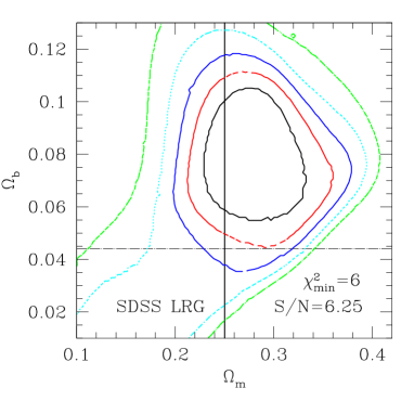
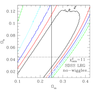
Left panel of Fig.8 shows the $\chi^{2}$ fit for $\Omega_{B}-\Omega_{m}$ plane using 9 singular values with a total signal-to-noise of $6.25$. We fix $h=0.7$ and marginalized over spectral index $n_{s}=0.8-1.2$ and biasing parameters $b_{1}=1.7-2.2$ and $c_{2}=0.0-5.0$. In the right panel we show the same fit for the EH models with no-wiggles (ie no BAO peak). Note how the values of $\Omega_{B}-\Omega_{m}$ become degenerate, as expected from our previous argument that the BAO peak helps to break the $\Omega_{B}-\Omega_{m}$ degeneracy. The best fit value without BAO peak is $\chi^{2}=11$ as opposed to $\chi^{2}=6$ with the BAO peak. Thus, in relative terms the models with and without a BAO peak are between 2 and 3-sigma away. But note that in absolute terms, models without the BAO peak are ruled out with $>99\%$ confidence.

The WMAP5 best fit value (marked by a cross) is outside the (2D) 1-sigma join region, but inside the (2D) 2-sigma contours. The best fit value is for $\Omega_{B}=0.079\pm 0.025$ and we find that $\Omega_{B}>0.035$ at 2-sigma level for any value of $\Omega_{m}$.

If we fix the $\Omega_{B}-\Omega_{m}$ to its best fit value, we find $b_{1}=1.7-2.2$ and $c_{2}=0.75-3.55$. The value of the linear bias $b_{1}$ is in excellent agreement with what we found in Paper I by fitting redshift space distortions in the 2-point function, but the error here is larger. The value of the non-linear bias $c_{2}\simeq 2$ is higher than the one we found in previous section for halos $c_{2}^{h}\simeq 0.2$. This is not surprising as it is well known that more than one LRG can occupy a single halo, in which case $c_{2}$ tends to be larger for a given $b_{1}$ Scoccimarro et al. (2001b). Also note that a larger value of $c_{2}$ makes the $Q_{3}$ signal-to-noise larger in the LRG data than in the MICE7680 group mocks. This helps defeating the shot-noise and improves the significance of the BAO detection.

V Conclusions

We have studied the large scale 3-point correlation function for luminous red galaxies from SDSS, and particularly the reduced $Q_{3}=\xi_{3}/\xi_{2}^{2}$, which measures the scaling expected from non-linear couplings. We find a well-detected peak at 105Mpc/h separation that is in agreement with the predicted position of BAO peak. This detection is significant since it is also imprinted in $\xi_{2}$ and $\xi_{3}$ separately. We focus our interpretation in $Q_{3}$ because it is a measure independent of time, $\sigma_{8}$ or growth factor. It only depends on the shape of the initial 2-point function and the non-linear coupling of the gravitational interaction. Our result for $Q_{3}$ is in excellent agreement with predictions from Gaussian initial conditions. When we use the $Q_{3}$ data alone (with no fit to the 2-point function) we are able to break the strong degeneracy between $\Omega_{m}$ and $\Omega_{B}$ (see Fig.8). Our detection shows a clear preference for a high value of $\Omega_{B}=0.079\pm 0.025$. This value is larger, but still consistent at 2-$\sigma$ with recent results of WMAP ($\Omega_{B}=0.045$). At 3-sigma level, the $\Omega_{m}-\Omega_{B}$ becomes degenerate. Models with no BAO peak are ruled out at 99% confidence level.

We have used very large realistic mock simulations to study the errors. These simulations show that $Q_{3}$ is not significantly modified in redshift space so we can use real-space perturbation theory (see Fig.2). This agreement also indicates that loop corrections are small on BAO scales Bernardeau et al. (2008). This analysis is independent from 2-point statistics, which tests the linear growth of gravity, since 3-point statistics test the non-linear growth. A high value for $\Omega_{B}$ is also consistent with the analysis of the peak in the 2-point correlation function shown in Eisenstein et al. (2005) and in Paper IV (Gaztanaga et al. (2008)) of this series, which detect a slightly higher peak than expected. We have done all the analysis with just one set of triangle configurations, with fixed sides of $r_{12}=33\pm 5.5$ Mpc/h and $r_{13}=88\pm 5.5$ Mpc/h, to center our attention to BAO scale. This is about optimal, but we notice that there is much more to learn from $Q_{3}$, which will be presented in future analysis. Results on smaller scales are consistent with what we find here.

Data is in excellent agreement with Gaussian initial conditions, for which $Q_{3}=0$. But note that our quadratic bias detection $c_{2}=0.75-3.55$ is degenerate with a primordial non-Gaussian (hierarchical) contribution. Indeed the mean value of $c_{2}\simeq 2$ seems larger in observations than in halo simulations, for which we find $c_{2}^{h}\simeq 0.2$. We believe that this indicates that halos are sometimes occupied by more than one galaxy, which increases the effective value of $c_{2}$ Scoccimarro et al. (2001b). But if we are conservative we can not rule out a primordial non-Gaussian contribution in the range $Q_{3}(Primordial)=c_{2}-c_{2}^{h}=[0.55,3.35]$.

Note that we have pixelized our data in cubical cells of side $dr=11$ Mpc/h. This results in some lost of small scale information but allows for a very fast method to estimate 3-point function Barriga and Gaztañaga (2002). This is important for data, but more for simulations. In the MICE7680 simulation there are close to $N=10^{11}$ particles. A brute force method to estimate 3-point correlation would require $N^{3}=10^{33}$ operations, while our method based on pixels just needed $5\times 10^{12}$ operations.

Figure 9: Same as Fig.4 for a future photometric Survey with photo-z error of $\Delta z<0.003(1+z)$, volume of $V=10Gpc^{3}/h^{3}$ and number density of $\bar{n}=10^{-3}h^{3}/Mpc^{3}$ LRG galaxies.

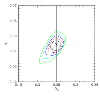
Future surveys will be able to improve much upon our measurement here. A photometric survey with $\Delta z<0.003(1+z)$ precision (corresponding to $dr<9$ Mpc/h at z=0), such as in the PAU Survey Benitez et al. (2008) should have enough spatial resolution to measure $Q_{3}(\alpha)$ as presented in this paper (recall that we are binning our radial distances in $dr=11$ Mpc/h). Such survey could sample over 10 times the SDSS DR6 volume (ie to z=0.9) with 20 times better LRG number density (ie for $L>L_{*}$). Fig.9 shows the forecast for such a survey, which we have simulated with the MICE7680 mocks in redshift space with a photo-z of $\Delta z<0.003(1+z)$ and for the same triangles as shown in our SDSS analysis. This is just illustrative, as we have not marginalized over biasing and other cosmological uncertainties. But note that the improvement is substantial and shows the potentiality of this method to constrain cosmological parameters and models of structure formation.

EG wish to thank Bob Nichol for suggesting the test with the EH no-wiggle model. We acknowledge the use of simulations from the MICE consortium (www.ice.cat/mice) developed at the MareNostrum supercomputer (www.bsc.es) and with support form PIC (www.pic.es), the Spanish Ministerio de Ciencia y Tecnologia (MEC), project AYA2006-06341 with EC-FEDER funding, Consolider-Ingenio PAU project CSD2007-00060 and research project 2005SGR00728 from Generalitat de Catalunya. AC acknowledge support from the DURSI department of the Generalitat de Catalunya and the European Social Fund.

References

- Bernardeau et al. (2002) F. Bernardeau, S. Colombi, E. Gaztañaga, and R. Scoccimarro, PhysRev 367, 1 (2002), eprint arXiv:astro-ph/0112551.
- Peebles and Groth (1975) P. J. E. Peebles and E. J. Groth, ApJ 196, 1 (1975).
- Fry and Peebles (1978) J. N. Fry and P. J. E. Peebles, ApJ 221, 19 (1978).
- Baumgart and Fry (1991) D. J. Baumgart and J. N. Fry, ApJ 375, 25 (1991).
- Gaztanaga (1992) E. Gaztanaga, ApJ 398, L17 (1992).
- Bouchet et al. (1993) F. R. Bouchet, M. A. Strauss, M. Davis, K. B. Fisher, A. Yahil, and J. P. Huchra, ApJ 417, 36 (1993), eprint arXiv:astro-ph/9305018.
- Fry and Gaztanaga (1994) J. N. Fry and E. Gaztanaga, ApJ 425, 1 (1994), eprint arXiv:astro-ph/9305032.
- Frieman and Gaztanaga (1994) J. A. Frieman and E. Gaztanaga, ApJ 425, 392 (1994), eprint arXiv:astro-ph/9306018.
- Jing and Boerner (1998) Y. P. Jing and G. Boerner, ApJ 503, 37 (1998), eprint arXiv:astro-ph/9802011.
- Frieman and Gaztañaga (1999) J. A. Frieman and E. Gaztañaga, ApJ 521, L83 (1999), eprint arXiv:astro-ph/9903423.
- Feldman et al. (2001) H. A. Feldman, J. A. Frieman, J. N. Fry, and R. Scoccimarro, Physical Review Letters 86, 1434 (2001), eprint arXiv:astro-ph/0010205.
- Colless et al. (2001) M. Colless, G. Dalton, S. Maddox, W. Sutherland, P. Norberg, S. Cole, J. Bland-Hawthorn, T. Bridges, R. Cannon, C. Collins, et al., MNRAS 328, 1039 (2001), eprint arXiv:astro-ph/0106498.
- York et al. (2000) D. G. York, J. Adelman, J. E. Anderson, Jr., S. F. Anderson, J. Annis, N. A. Bahcall, J. A. Bakken, R. Barkhouser, S. Bastian, E. Berman, et al., AJ 120, 1579 (2000), eprint arXiv:astro-ph/0006396.
- Colombi et al. (1998) S. Colombi, I. Szapudi, and A. S. Szalay, MNRAS 296, 253 (1998), eprint arXiv:astro-ph/9711087.
- Szapudi et al. (1999) I. Szapudi, S. Colombi, and F. Bernardeau, MNRAS 310, 428 (1999), eprint arXiv:astro-ph/9912289.
- Matarrese et al. (1997) S. Matarrese, L. Verde, and A. F. Heavens, MNRAS 290, 651 (1997), eprint arXiv:astro-ph/9706059.
- Scoccimarro et al. (2004) R. Scoccimarro, E. Sefusatti, and M. Zaldarriaga, PRD 69, 103513 (2004), eprint arXiv:astro-ph/0312286.
- Sefusatti and Scoccimarro (2005) E. Sefusatti and R. Scoccimarro, PRD 71, 063001 (2005), eprint arXiv:astro-ph/0412626.
- Gaztañaga et al. (2005) E. Gaztañaga, P. Norberg, C. M. Baugh, and D. J. Croton, MNRAS 364, 620 (2005), eprint arXiv:astro-ph/0506249.
- Nichol et al. (2006) R. C. Nichol, R. K. Sheth, Y. Suto, A. J. Gray, I. Kayo, R. H. Wechsler, F. Marin, G. Kulkarni, M. Blanton, A. J. Connolly, et al., MNRAS 368, 1507 (2006), eprint arXiv:astro-ph/0602548.
- Kayo et al. (2004) I. Kayo, Y. Suto, R. C. Nichol, J. Pan, I. Szapudi, A. J. Connolly, J. Gardner, B. Jain, G. Kulkarni, T. Matsubara, et al., PASJ 56, 415 (2004), eprint arXiv:astro-ph/0403638.
- Nishimichi et al. (2007) T. Nishimichi, I. Kayo, C. Hikage, K. Yahata, A. Taruya, Y. P. Jing, R. K. Sheth, and Y. Suto, PASJ 59, 93 (2007), eprint arXiv:astro-ph/0609740.
- Kulkarni et al. (2007) G. V. Kulkarni, R. C. Nichol, R. K. Sheth, H.-J. Seo, D. J. Eisenstein, and A. Gray, MNRAS 378, 1196 (2007), eprint arXiv:astro-ph/0703340.
- Sefusatti and Komatsu (2007) E. Sefusatti and E. Komatsu, PRD 76, 083004 (2007), eprint arXiv:0705.0343.
- Fry and Gaztanaga (1993) J. N. Fry and E. Gaztanaga, ApJ 413, 447 (1993), eprint arXiv:astro-ph/9302009.
- Fry (1994) J. N. Fry, Physical Review Letters 73, 215 (1994).
- Scoccimarro et al. (2001a) R. Scoccimarro, H. A. Feldman, J. N. Fry, and J. A. Frieman, ApJ 546, 652 (2001a), eprint arXiv:astro-ph/0004087.
- Verde et al. (2002) L. Verde, A. F. Heavens, W. J. Percival, S. Matarrese, C. M. Baugh, J. Bland-Hawthorn, T. Bridges, R. Cannon, S. Cole, M. Colless, et al., MNRAS 335, 432 (2002), eprint arXiv:astro-ph/0112161.
- Cabré and Gaztañaga (2008a) A. Cabré and E. Gaztañaga, MNRAS in press 2460 (2008a), eprint 0807.2460.
- Cabré and Gaztañaga (2008b) A. Cabré and E. Gaztañaga, ArXiv e-prints 2461 (2008b), eprint 0807.2461.
- Eisenstein et al. (2005) D. J. Eisenstein, I. Zehavi, D. W. Hogg, R. Scoccimarro, M. R. Blanton, R. C. Nichol, R. Scranton, H.-J. Seo, M. Tegmark, Z. Zheng, et al., ApJ 633, 560 (2005), eprint arXiv:astro-ph/0501171.
- Hütsi (2006) G. Hütsi, A&A 449, 891 (2006), eprint arXiv:astro-ph/0512201.
- Percival et al. (2007) W. J. Percival, S. Cole, D. J. Eisenstein, R. C. Nichol, J. A. Peacock, A. C. Pope, and A. S. Szalay, MNRAS 381, 1053 (2007), eprint arXiv:0705.3323.
- Padmanabhan et al. (2007) N. Padmanabhan, D. J. Schlegel, U. Seljak, A. Makarov, N. A. Bahcall, M. R. Blanton, J. Brinkmann, D. J. Eisenstein, D. P. Finkbeiner, J. E. Gunn, et al., MNRAS 378, 852 (2007), eprint arXiv:astro-ph/0605302.
- Blake et al. (2007) C. Blake, A. Collister, S. Bridle, and O. Lahav, MNRAS 374, 1527 (2007), eprint arXiv:astro-ph/0605303.
- Barriga and Gaztañaga (2002) J. Barriga and E. Gaztañaga, MNRAS 333, 443 (2002), eprint arXiv:astro-ph/0112278.
- Gaztañaga and Scoccimarro (2005) E. Gaztañaga and R. Scoccimarro, MNRAS 361, 824 (2005), eprint arXiv:astro-ph/0501637.
- Hui and Gaztañaga (1999) L. Hui and E. Gaztañaga, ApJ 519, 622 (1999), eprint arXiv:astro-ph/9810194.
- Gaztanaga et al. (2008) E. Gaztanaga, A. Cabre, and L. Hui, ArXiv e-prints 807 (2008), eprint 0807.3551.
- Groth and Peebles (1977) E. J. Groth and P. J. E. Peebles, ApJ 217, 385 (1977).
- Peebles (1980) P. J. E. Peebles, The large-scale structure of the universe (Research supported by the National Science Foundation. Princeton, N.J., Princeton University Press, 1980. 435 p., 1980).
- Gaztañaga and Lobo (2001) E. Gaztañaga and J. A. Lobo, ApJ 548, 47 (2001), eprint arXiv:astro-ph/0003129.
- Gaztanaga (1994) E. Gaztanaga, MNRAS 268, 913 (1994), eprint arXiv:astro-ph/9309019.
- Gaztanaga and Frieman (1994) E. Gaztanaga and J. A. Frieman, ApJ 437, L13 (1994), eprint arXiv:astro-ph/9407079.
- Sefusatti et al. (2006) E. Sefusatti, M. Crocce, S. Pueblas, and R. Scoccimarro, PRD 74, 023522 (2006), eprint arXiv:astro-ph/0604505.
- Eisenstein and Hu (1998) D. J. Eisenstein and W. Hu, ApJ 496, 605 (1998), eprint arXiv:astro-ph/9709112.
- Sanchez et al. (2008) A. G. Sanchez, C. M. Baugh, and R. Angulo, ArXiv e-prints 804 (2008), eprint 0804.0233.
- Evrard et al. (2008) A. E. Evrard, J. Bialek, M. Busha, M. White, S. Habib, K. Heitmann, M. Warren, E. Rasia, G. Tormen, L. Moscardini, et al., ApJ 672, 122 (2008), eprint arXiv:astro-ph/0702241.
- Scoccimarro et al. (2001b) R. Scoccimarro, R. K. Sheth, L. Hui, and B. Jain, ApJ 546, 20 (2001b), eprint arXiv:astro-ph/0006319.
- Szapudi (2004) I. Szapudi, ApJ 605, L89 (2004), eprint arXiv:astro-ph/0404476.
- Eisenstein et al. (2001) D. J. Eisenstein, J. Annis, J. E. Gunn, A. S. Szalay, A. J. Connolly, R. C. Nichol, N. A. Bahcall, M. Bernardi, S. Burles, F. J. Castander, et al., AJ 122, 2267 (2001), eprint arXiv:astro-ph/0108153.
- Schlegel et al. (1998) D. J. Schlegel, D. P. Finkbeiner, and M. Davis, ApJ 500, 525 (1998), eprint arXiv:astro-ph/9710327.
- Swanson et al. (2008) M. E. C. Swanson, M. Tegmark, M. Blanton, and I. Zehavi, MNRAS 385, 1635 (2008), eprint arXiv:astro-ph/0702584.
- Blanton et al. (2005) M. R. Blanton, D. J. Schlegel, M. A. Strauss, J. Brinkmann, D. Finkbeiner, M. Fukugita, J. E. Gunn, D. W. Hogg, Ž. Ivezić, G. R. Knapp, et al., AJ 129, 2562 (2005), eprint arXiv:astro-ph/0410166.
- Górski et al. (2005) K. M. Górski, E. Hivon, A. J. Banday, B. D. Wandelt, F. K. Hansen, M. Reinecke, and M. Bartelmann, ApJ 622, 759 (2005), eprint arXiv:astro-ph/0409513.
- Bernardeau et al. (2008) F. Bernardeau, M. Crocce, and R. Scoccimarro, ArXiv e-prints 806 (2008), eprint 0806.2334.
- Benitez et al. (2008) N. Benitez, E. Gaztanaga, R. Miquel, F. Castander, M. Moles, M. Crocce, A. Fernandez-Soto, P. Fosalba, F. Ballesteros, J. Campa, et al., ArXiv e-prints 807 (2008), eprint 0807.0535.