Knowledge Acquisition by Networks of Interacting Agents
in the Presence of Observation Errors

Abstract

In this work we investigate knowledge acquisition as performed by multiple agents interacting as they infer, under the presence of observation errors, respective models of a complex system. We focus the specific case in which, at each time step, each agent takes into account its current observation as well as the average of the models of its neighbors. The agents are connected by a network of interaction of Erdős-Rényi or Barabási-Albert type. First we investigate situations in which one of the agents has a different probability of observation error (higher or lower). It is shown that the influence of this special agent over the quality of the models inferred by the rest of the network can be substantial, varying linearly with the respective degree of the agent with different estimation error. In case the degree of this agent is taken as a respective fitness parameter, the effect of the different estimation error is even more pronounced, becoming superlinear. To complement our analysis, we provide the analytical solution of the overall behavior of the system. We also investigate the knowledge acquisition dynamic when the agents are grouped into communities. We verify that the inclusion of edges between agents (within a community) having higher probability of observation error promotes the loss of quality in the estimation of the agents in the other communities.

‘Knowledge is of two kinds: we know a subject ourselves, or we know where we can find information upon it.’ (S. Johson)

I Introduction

Several important systems in nature, from the brain to society, are characterized by intricate organization. Being naturally related to such systems, humans have been trying to understand them through the construction of models which can reasonably reproduce and predict the respectively observed properties. Model building is the key component in the scientific method. The development of a model involves the observation and measurement of the phenomenon of interest, its representation in mathematical terms, followed by simulations and respective confrontation with further experimental evidences. Because of the challenging complexity of the remaining problems in science, model building has become intrinsically dependent on collaboration between scientists or agents. The problem of multiple-agent knowledge acquisition and processing has been treated in the literature (e.g.  Botti et al. (1993); Sajja (2008)), but often under assumption of simple schemes of interactions between the agents (e.g. lattice or pool). Introduced recently, complex networks ( Albert and Barabási (2002); Dorogovtsev and Mendes (2002); Newman (2003); Boccaletti et al. (2006); da F. Costa et al. (2007)) have quickly become a key research area mainly because of the generality of this approach to represent virtually any discrete system, allied to the possibilities of relating network topology and dynamics. As such, complex networks stand out as being a fundamental resource for complementing and enhancing the scientific method.

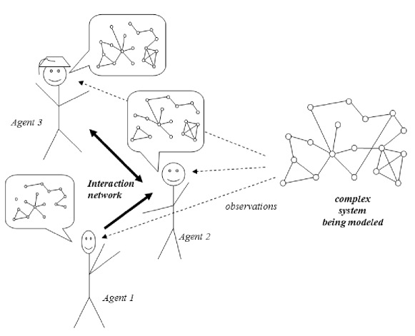
The present study addresses the issue of modeling how one or more agents (e.g. scientists) progress while modeling a complex system. We start by considering a single agent and then proceed to more general situations involving several agents interacting through networks of relationships (see Figure 1). The agents investigating the system (one or more) are allowed to make observations and take measurements of the system as they develop and complement their respective individual models. Errors, incompleteness, noise and forgetting are typically involved during a such model estimation. The main features of interest include the quality of the obtained models and the respective amount of time required for their estimation. The plural in ‘models’ stands for the fact that the models obtained respectively by each agent are not necessarily identical and will often imply in substantial diversity. Though corresponding to a largely simplified version of real scientific investigation, our approach captures some of the main elements characterizing the involvement of a large number of interacting scientists who continuously exchange information and modify their respective models and modeling approaches. As a matter of fact, in some cases the development of models may even affect the system being modeled (e.g. the perturbation implied by the measurements on the analyzed systems).

Figure 1: Agents (scientists) develop their models of complex systems through observation and interactions.

Because interactions between scientists can be effectively represented in terms of complex networks (e.g. de Solla Price (1965); Newman (2001a, b, c); Moody (2004); Barabási et al. (2002); Silva et al. (2007)), it is natural to resource to such an approach in our investigation. It is interesting to observe that the agents may not be limited to scientists, but can also include intelligent machines and even reference databases and libraries. Though most of the previous approaches to modeling scientific interaction in terms of complex networks have focused on the topology of the collaborations, fewer strategies (e.g. da F. Costa (2006)) have addressed the important issue of how the dynamics of learning/knowledge acquisition evolves in such systems, especially with respect to distinct patterns of connectivity between the agents. This is the main motivation of the current work.

This article starts by presenting the general assumptions and specifying and discussing successively more sophisticate levels of modeling. We then focus on the development of a model of a complex system by a team of agents interacting through networks of Erdős-Rényi (ER) and Barabási-Albert (BA) types. During estimation, each agent takes into account not only its observation (subject to a probability of error), but also the average of the models of its neighbors. In order to quantify the performance of an agent, we suggest an individual error based on the difference between the model developed and the system under analysis. Because the influence of an agent is directly related to its degree, the overall error of the system is expressed in terms of the mean of the individual errors weighted by the degree of each respective agent. The obtained results imply a series of interesting and important insights, such as the identification of the substantial role of hubs in affecting the estimation of models by all agents: while a linear relationship is identified between the overall estimation errors and the degree of single agents with different error rates, this relationship becomes superlinear when the degree of each node is considered as the respective fitness. In addition, in networks characterized by presence of communities, intensifying the interactions between agents having higher estimation errors in one of the communities undermines the performance of the agents in the other communities.

II General Assumptions

The first important assumption is that the complex systems under study be representable as a discrete structure (e.g. a graph or complex network), and that information about the several parts of this system can be observed, often with a given probability of error. By agent, it is meant any entity capable of making observations/measurements of the system under analysis and storing this information for some period of time. Therefore, any scientist can be naturally represented as an agent. However, automated systems, from measurement stations to more sophisticated reasoning systems, can also be represented as agents. Actually, even less dynamic systems such as books or libraries can be thought of as a sort of passive agents, in the sense that they evolve (new editions and versions) as a consequence of incorporation of the evolution of knowledge.

Each agent is capable of making observations/measurements of the system under investigation. The process of measurement typically involves errors, which can be of several types such as observing a connection where there is none. Such errors can be a direct consequence of the limited accuracy of measurements devices as well as of the priorities and eventual biases (not to mention wishful thinking) of each agent. Several other possibilities, such as the existence of non-observable portions of the system, can also be considered and incorporated into the model. In addition, the model kept by each agent may undergo degradation as a consequence of noise and/or vanishing memory.

A particularly important element in our approach is the incorporation of different types of interactions between the agents, which can be represented in terms of a graph or network (see Figure 1). In this case, each agent gives rise to a node, while interactions (e.g. collaborations) among them are represented by links. The single-agent configuration can be immediately thought of as a special case where the graph involves only one node (agent). Several types of interactions are possible including, but being not limited to conversations, attendance to talks or courses (the speaker becomes a temporary hub), article/book, reading, and Internet exchanges (e.g. e-mailing and surfing). Such interactions may also involve errors (e.g. misunderstanding words during a talk), which can be eventually incorporated into our model. It is interesting to observe that the network of interaction between the agents may present dynamic topology, varying with time as a consequence of new scientific partnerships, addition or removal of agents, and so on.

Therefore, the framework considered in our investigation includes the following three basic components: (i) the complex system under analysis $S$; (ii) one or more agents capable of taking observations/measurements of the system $S$ (subject to error) and of interacting one another; (iii) a network of interaction between the agents. In the following we address, in progressive levels of sophistication, the modeling of knowledge acquisition/model building in terms of complex networks concepts and tools.

III Single-Agent Modeling

A very simple situation would be the case where a single agent is allowed to observe, in uniformly random fashion, the presence or not of connections between all pairs of nodes of the complex system being modeled. The observation of each edge involves a probability $\gamma$ of error, i.e. observing a connection where there is none and vice-versa. A possible procedure of model building adopted by the agent involves taking the average of all individual observations up to the current time step $T$ , i.e.

$$\left<x\right>_{T}=\frac{1}{T}\sum_{t=1}^{T}x_{t},$$ (1)

where $x$ is the value of a specific edge (0 if non-existent and 1 otherwise)and $x_{t}$ is the observation of $x$ at time step $t$. Observe that we are considering the observation error to be independent along the whole system under analysis. Let us quantify the error for estimation of any edge, after $T$ time steps as follows

$$\epsilon(x)_{T}=\left|x_{*}-\left<x\right>_{T}\right|,$$ (2)

where $x_{*}$ is the original value of that edge. It can be easily shown that

$$\lim_{T\rightarrow\infty}\epsilon(x)_{T}=\gamma$$ (3)

Because the observation error is independent among the pairs of nodes, the average of the errors along the whole network is identical to the limit above.

Thus, in this configuration the best situation which can be aimed at by the agent is to reach a representation of the connectivity of the original complex system up to an overall limiting error $\gamma$, reached after a considerable period of time. Though the speed of convergence is an interesting additional aspect to be investigated while modeling multi-agent knowledge acquisition, we leave this development for a forthcoming investigation.

IV Multiple-Agent Modeling

We now turn our attention to a more interesting configuration in which a total of $N_{a}$ agents interact while making observations of the complex system under analysis, along a sequence of time steps. As before, each agent observes the whole system at each time step, with error probability $\gamma$. In case no communication is available between the agents, each one will evolve exactly as discussed in the previous section. However, our main interest in this work is to investigate how interactions and influences between the multiple agents can affect the quality and speed at which the system of interest is learned. The original system under study is henceforth represented in terms of its respective adjacency matrix $A_{*}$. We also assume that the agents exchange information through a complex network of contacts.

One of the simplest, and still interesting, modeling strategies to be adopted by the agents of such a system involves the following dynamics: at each time step $t$, each of the agents $i$ observes the connectivity of the complex system with error $\gamma$, yielding the adjacency matrix $O_{i}^{t}$, and also receives the current matrices from each of its immediate neighbors$j$ (i.e. the agents to which it is directly connected). The agent $i$ then calculates the mean matrix $\left<K\right>^{t}$ of the matrices $K_{ji}^{t}$ received from all its neighbors $j$, i.e.

$$~{}\left<K\right>^{t}=\frac{1}{k_{i}}\sum_{j}K_{ji}^{t},$$ (4)

where $k_{i}$ is the degree of the agent $i$. The agent $i$ then makes a weighted average between its current matrix $K_{i}^{t}$ and the immediate neighbors mean matrix, i.e.

$$v_{i}^{t}=(a\left<K\right>^{t}+(1-a)K_{i}^{t}),$$ (5)

where $0<a\leq 1$ is a relative weight. We henceforth assume $a=0.5$, so that $v_{i}^{t}$ becomes equal to the average between its current matrix and of the neighbors at that time step. Each agent $i$ subsequently adds this value to its current observation, i.e.

$$K_{i}^{(t+1)}=v_{i}^{(t)}+O_{i}^{(t)},$$ (6)

so after $T$ time steps the estimation of the adjacency matrix by the agent $i$ can be given as

$$A_{i}^{(T)}=K_{i}^{(T)}/T.$$ (7)

This simple discrete-type dynamics has some immediate important consequences. Because each node receives estimations from its neighbors at each time step, an altered quality of estimation is obtained. Indeed, by averaging between its current observation and the mean estimation from the neighbors, even the limit error may be actually modified with respect to the single agent situation.

Several variations and elaborations of this model are possible, including the consideration of noise while transmitting the observations between adjacent agents, forgetting, the adoption of other values of $a$, as well as other averaging and noise schemes. In this article, however, we focus attention on the multi-agent model described in this section with error being present only during the observation by each agent. In the remainder of our work, we report results of numerical simulation considering three particularly important situations: (i) multiple-agents with equal observation errors; (ii) as in (i) but with one of the agents having different observation error; and (iii) multiple-agents scheme applied in networks with community structure and one of the communities having higher error rate. Interesting results are obtained for all these three configurations including the analytical solution of the overall behavior of the system.

V Case Examples: Random and Scale-Free Networks of Agents

In this section we investigate further the dynamics of multi-agent learning by considering theoretical simulations performed with a fixed collaboration network. We assume that the agents collaborate through a uniformly random model (ER) as well as a scale-free model (BA), both containing 50 nodes and average degree equal to 9.4. For simplicity’s sake, we consider only a single realization of such a model in our subsequent investigation. The performance of each agent is quantified in terms of the error between the original network and the models obtained by that agent after a sufficiently large number of time steps (henceforth assumed to be equal to $T=300$ time steps). This error is calculated as

$$\varepsilon_{p}^{(T)}=\frac{1}{N^{2}}\sum_{m=1}^{N}\sum_{n=1}^{N}|A_{i}^{(T,m,n)}-A_{*}^{m,n}|$$ (8)

where $A_{i}$ is the adjacency matrix representation of the model of agent $i$ at time step $T$. The original network to be learnt by the agents is a Barabási-Albert network containing $N=50$ nodes and average degree equal to 6, represented by the respective adjacency matrix $A_{*}$. The overall performance of the network, including all its agents, is henceforth expressed in terms of the average of the above error weighted by the degree considering all agents, which is here called the overall error of the system:

$$E^{(T)}=\frac{1}{\sum_{i=1}^{N_{a}}k_{i}}\sum_{i=1}^{N_{a}}k_{i}\varepsilon_{i}^{T}$$ (9)

Because the influence of an agent in the network is correlated with the number of its neighbors, such a definition of the overall error takes into account the respective importance of the models of each agent.

V.1 Analytical Description

We now present the mathematical formalization of the above concepts. We start with the difference equation that characterizes the dynamics of each agent $i$:

$$2K_{i}^{t+1}=\left[\frac{1}{k_{i}}\sum_{j\in\Gamma}K_{j}^{t}\right]+K_{i}^{t}+2O_{i}^{t}$$ (10)

where $K_{i}^{t}$ is the current matrix and $O_{i}^{t}$ is the observation of the agent $i$ at time step $t$. The term in brackets is the mean of the matrices received from the set $\Gamma$ of the neighbors of $i$. Now we consider the continuous approximation given by:

$$2\frac{d}{dt}K_{i}(t)=\left[\frac{1}{k_{i}}\sum_{j\in\Gamma}K_{j}(t)\right]-K_{i}(t)+2O_{i}(t)$$ (11)

Dividing by $t$ and knowing that $\frac{1}{t}\frac{d}{dt}K_{i}(t)=\frac{d}{dt}\left(\frac{K_{i}^{t}}{t}\right)+\frac{1}{t^{2}}K_{i}^{t}$, we have

$$2k_{i}\frac{d}{dt}\left[\frac{K_{i}(t)}{t}\right]+2k_{i}\frac{K_{i}(t)}{t^{2}}=\\ =\left[\sum_{j\in\Gamma}\frac{K_{j}(t)}{t}\right]-k_{i}\frac{K_{i}(t)}{t}+2k_{i}\frac{O_{i}(t)}{t}$$ (12)

and adding, for every agent $i$ :

$$\frac{d}{dt}\sum_{i=1}^{N_{a}}\left[\frac{k_{i}K_{i}(t)}{t}\right]=\\ \frac{1}{t}\sum_{i=1}^{N_{a}}k_{i}O_{i}(t)-\frac{1}{t}\sum_{i=1}^{N_{a}}\left[\frac{k_{i}K_{i}(t)}{t}\right]$$ (13)

since $\sum_{i}\sum_{j\in\Gamma}\frac{K_{j}(t)}{t}=\sum_{i}\frac{k_{i}K_{i}(t)}{t}$. Finally, we define $J\equiv\sum_{i}\frac{k_{i}K_{i}(t)}{t}$:

$$~{}\frac{d}{dt}J(t)=\frac{1}{t}\sum_{i=1}^{N}k_{i}O_{i}(t)-\frac{1}{t}J(t)$$ (14)

For an agent $i$ the probability of observing an edge where there is none and vice-versa is $\gamma_{i}$. So, for an entry $A_{*}^{m,n}$ of the system under observation:

$$\lim_{T\rightarrow\infty}\left[\frac{1}{T}\int\left(\sum_{i}k_{i}O_{i}^{m,n}(t)\right)dt\right]=\\ =\left\{\begin{array}[]{lc}\sum_{i}k_{i}(1-\gamma_{i})&\mbox{if}\quad A_{*}^{m,n}=1\\ \vskip 6.0pt plus 2.0pt minus 2.0pt\cr\sum_{i}k_{i}(\gamma_{i})&\mbox{if}\quad A_{*}^{m,n}=0\end{array}\right.$$ (15)

Applying this result in equation  14 and solving, we have :

$$\lim_{T\rightarrow\infty}J^{m,n}(T)=\left\{\begin{array}[]{lc}\sum_{i}k_{i}(1-\gamma_{i})&\mbox{if}\quad A_{*}^{m,n}=1\\ \vskip 6.0pt plus 2.0pt minus 2.0pt\cr\sum_{i}k_{i}(\gamma_{i})&\mbox{if}\quad A_{*}^{m,n}=0\end{array}\right.$$ (16)

and subtracting $\sum_{i}k_{i}A_{*}^{m,n}$ and adding for all m and n

$$\sum_{m=1}^{N}\sum_{n=1}^{N}\left(J^{m,n}(T)-\sum_{i}k_{i}A_{*}^{m,n}\right)=\\ =\sum_{i}\left(\sum_{m=1}^{N}\sum_{n=1}^{N}\gamma_{i}k_{i}\right)$$

$$\Rightarrow\sum_{i=1}^{Na}\left[\frac{k_{i}}{N^{2}}\left(\frac{K_{i}^{T}}{T}-A_{*}\right)\right]=\sum_{i=1}^{N_{a}}k_{i}\gamma_{i}$$ (17)

for both cases. The term in the sum is precisely the individual error of an agent $i$ weighted by its degree. Then, dividing by the sum of the degrees, we have the analytical expression for the overall error of the system.

$$\frac{\sum_{i=1}^{Na}k_{i}\varepsilon_{i}}{\sum_{i}k_{i}}=\frac{\sum_{i=1}^{Na}k_{i}\gamma_{i}}{\sum_{i}k_{i}}$$

$$\Rightarrow E^{T}=\frac{1}{\left<k\right>N_{a}}\sum_{i=1}^{N_{a}}k_{i}\gamma_{i}$$ (18)

We can apply this result in two following situations, assuming a network of agents with average degree $\left<k\right>$ and maximum and minimum degree equal to $max_{d}$ and $min_{d}$, respectively:

a) One agent $j$ with degree $k_{j}$ having an observation error $\gamma_{j}=p\gamma$ and all other agents with an error rate $\gamma$:

$$E^{T}=\frac{\left(\sum_{i=1}^{N_{a}}{k_{i}\gamma}\right)-\gamma k_{j}+p\gamma k_{j}}{\left<k\right>N_{a}}$$

$$\Rightarrow E^{T}=\frac{k_{j}\gamma(p-1)}{\left<k\right>N_{a}}+\gamma$$ (19)

which is a linear relation with respect to the degree of the agent with different error rate. Note that, there is no difference between any two networks of agents with the same average degree and number of vertices.

b) One agent $j$ with degree $k_{j}$ having an observation error proportional to its degree $\gamma_{j}(\gamma\geq\gamma_{j}\geq 1)$ and all other agents with an error rate $\gamma$:

$$\Rightarrow E^{T}=\frac{k_{j}(1-\gamma)(k_{j}-min_{d})}{\left<k\right>N_{a}(max_{d}-min_{d})}+\gamma$$ (20)

which is a power-law relation with respect to the degree of the agent with different error rate.

V.2 Fixed Observation Errors

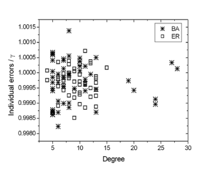
In this first configuration, all nodes have the same estimation error $\gamma=0.2$, and therefore the same influence, over the averages obtained by each agent. However, nodes with higher degree, especially hubs, are still expected to influence more strongly the overall dynamics as a consequence of the fact that their estimated models are taken into account by a larger number of neighbors. Figure 2 shows the distribution of the average of the errors $\varepsilon_{i}^{T}$ obtained for this case in terms of the respective degrees. As could be expected, the errors obtained among the agents are very similar one another. Thus, there is no major difference in the learning quality among the agents. A rather different situation arises in the next sections, where we consider different error rates.

Figure 2: The individual estimation errors in terms of the degree of the agents obtained for the Erdős-Rényi (ER) and Barabási-Albert (BA) models with $N_{a}=50$ and $\left<k\right>=9.4$.

V.3 Varying Observation Errors

We now repeat the previous configuration in two new situations: (i) one of the agents having half or twice the error rate of the others; and (ii) having an error proportional to its degree. Simulations are performed independently while placing the higher error rate at all of the possible nodes, while the respective overall errors are calculated. In addition, we compared the behavior for the Erdős-Rényi (ER) and Barabási-Albert (BA) network of agents.

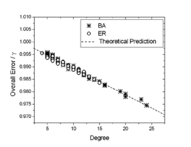
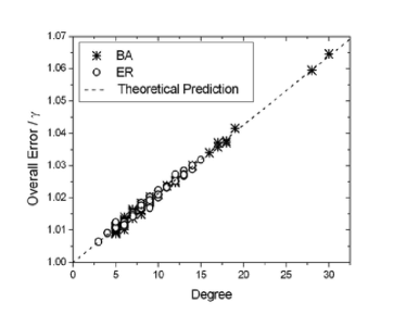
Figure 3(a) shows the results obtained while considering error probability equal to 0.2 for one of the agents and $\gamma=0.4$ for all other agents. It is possible to identify a substantial difference of the mean quality of the models which depends linearly on the degree of the node with different error rate. More specifically, it is clear that the overall errors are much smaller for nodes with higher degrees. In other words, the best models will be obtained when the hubs have smaller observation errors, influencing strongly the rest of the agents through the diffusion, along time, of their respectively estimated models.

Figure 3(b) shows the results obtained when the estimation error of one of the agents is $0.4$ while the rest of the agents have error rate $\gamma=0.2$. The opposite effect is verified, with the overall error increasing linearly with the degree of the node with higher estimation error. Moreover, as expected, no difference was found between the ER and BA models in both cases.

(a)                                                                       (b)

Figure 3: The overall estimation errors in terms of the degree of the agents with different error rates for ER and BA models: (a) one agent with an error rate equal to $0.2$ and all other agents with $\gamma=0.4$; and (b) one node with 0.4 and all other nodes with $\gamma=0.2$. The dashed line represents the analytical solution.

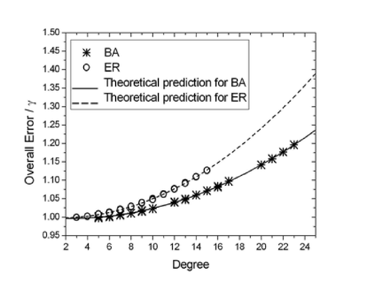
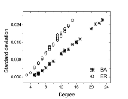
Figure 4 shows the results obtained when one of the agents has a higher error rate than the others, and proportional to its degree. Results similar to the previous case were found, but with a nonlinear behavior. In addition, accordingly with the analytical predictions, a separation was verified between the ER and BA networks (ER presents higher values than BA). This means that when we consider two nodes with the same degree, each in one network, the overall error is lower for the BA model, since their hubs influence more strongly the to increase the quality of the estimated models.

Figure 4: The overall estimation errors in terms of the degree of the agents with higher error rates: one agent with an error proportional to its degree and all other agents with $\gamma=0.2$. The dashed and straight lines represent the analytical solution for the ER and BA models, respectively.

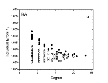
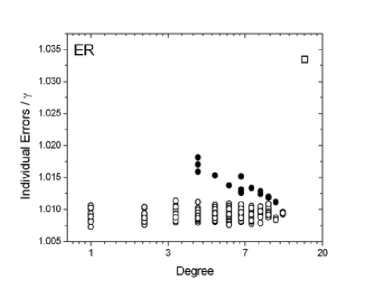
A better picture of the influence of the degree over the model development by other agents is provided in Figure 5 respectively to the situation having twice the error probability ($\gamma_{j}=0.4$) for the agent $j$ with the highest degree. Figures 5(a) and  5(c) consider the $\varepsilon_{i}^{T}$ of individual agents in terms of their respective degrees for the BA and ER models, respectively. It is clear from these results that the degree of the differentiated agent affects the estimation of the whole set of agents, especially for its neighborhood, shifting substantially the average individual errors. Observe also that, in both cases, the largest individual error results precisely at the less accurate agent. Furthermore, nodes with high degrees tend to be less influenced by the agent with different error rate.

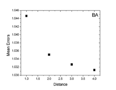
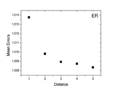
Figures  5(b) and  5(d) complement the analysis considering the mean value of the individual errors of agents with the same topological distance from the agent with different error probability. The results show that the closer agents tend to be more affected than the peripherals.

From the results above, we immediately verify that the presence of the less accurate agent produces a non-uniform error distribution. Since the individual error of an agent is produced by averaging between its model and the mean estimation from the neighbors, the direct contact (and proximity) with agents with higher error rates alters considerably its final model. Moreover, this effect is more strongly felt by agents with few connections.

(a)                                                                       (b)

(c)                                                                       (d)

Figure 5: The individual estimation errors in terms of the degree of the agents (a and c): $\square$, the agent with highest error rate; $\bullet$, the neighborhood of the agent with different error rate. Figures (b and d) show the mean value of the individual errors of a set of nodes with the same topological distance from the agent with higher error rate. Simulations for the ER and BA models with $N_{a}=300$ and $\left<k\right>=4.7$.

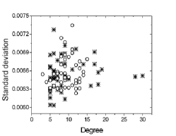
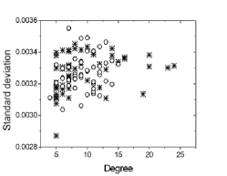
Figure 6 shows the standard deviation of individual errors in terms of the degrees of the agents with different error rate for the three situations above. Differently from the first two situations (figures  6(a) and  6(b)), we detected a positive correlation when one agent has an error rate proportional to its degree (figure  6(c)).

(a)                                             (b)                                             (c)

Figure 6: The standard deviation of individual errors in terms of the degree of the agents with different error rates: (a) one agent with $\gamma=0.2$ and all other agents with 0.4; (b) one node with $\gamma=0.4$ and all other nodes with 0.2; and (c) one agent with an error proportional to its degree and all other agents with 0.2.

V.4 Varying Observation Errors in Communities

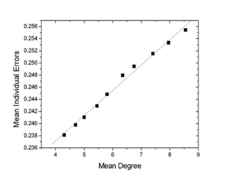
We also applied the knowledge acquisition dynamics to a network of agents with community structure. During the simulations all agents of one of the communities have twice the error rate of the others. We are interested in obtaining the correlations between the average degree of the community with higher error rate and the mean value of the individual errors of the agents of the other communities. Figure 7 shows the results for a network with $N_{a}=100$ agents and 5 communities of the same size. While the estimation error of one of the communities is 0.4, the agents of other communities have error 0.2. We find a positive correlation which means that the addition of edges between the agents with higher error rates increases the individual errors of the agents of the other communities.

This effect can be explained by the existence of bridging agents which belong to the community with higher error rate but connect to another clusters. Because the individual errors takes into account the models of the neighborhood, these special agents tend to reach worse models when the intra-community communication is intensified. Indeed, the addition of new edges implies more agents with higher errors to influence to the development of their estimations. Consequently, the loss of performance propagates to another communities.

Figure 7: Correlation between the average degree of the community of higher error rate and the mean value of the individual errors of the agents of the other communities.

VI Concluding Remarks

The important problem of scientific interaction has been effectively investigated in terms of concepts and tools of complex networks research (e.g.de Solla Price (1965); Newman (2001a, b, c); Moody (2004); Barabási et al. (2002)). However, most of the interest has been so far concentrated on characterizing the connectivity between scientists and institutions. The present study reported what is possibly the first approach to model the dynamics of knowledge acquisition (building a model of a complex system) by a system of multiple agents interacting through specific types of complex network. Several configurations were considered at increasing levels of sophistication. Each agent was assumed to make an observation of the system of interest at each time step with error probability $\gamma$.

A series of interesting and important results have been identified analytically and through simulations. First, we have that the individual estimation error tends to $\gamma$ when the agents do not interact one another. However, different individual errors were observed when the agents were allowed to consider the average of models at each of their immediate neighbors. Special attention was given to the cases in which one of the agents has a different observation error, yielding the important result that the overall error in such a configuration tends to be correlated with the degree of the agent with different observation error. More specifically, we demonstrated that this correlation is linear when one agent has an error half or twice the error rate of the others, and nonlinear when it is proportional to its degree. In other words, the connectivity will have a substantial influence over the models developed by the agents, for better or for worse. It is interesting to observe that agents with many connections will imply strong influences over the whole network even in case those agents have no special fitness. Such an effect is a direct consequence of the fact that those agents are heard by more people. In case the hubs have higher observation errors, worse models are obtained throughout the agents network. In particular, the negative influence of the hubs is more strongly felt by its neighborhood. Finally, we have shown that when the agents are clustered into communities, the addition of edges in the communities with different error rate leads to the change of the individual errors of the agents in the other groups.

This investigation has paved the way to a number of subsequent works, including but not being limited to: consideration of model degradation along time, other learning strategies, other types of networks, observation errors conditional to specific local features (e.g. degree or clustering coefficient) of the network being modeled, as well as other distribution of observation errors among the agents.