Treating the $b$ quark distribution function with reliable uncertainties

Abstract

The parton distribution function for a $b$ quark in the $B$ meson (called the shape function) plays an important role in the analysis of the $B\to X_{s}\gamma$ and $B\to X_{u}\ell\bar{\nu}$ data, and gives one of the dominant uncertainties in the determination of $|V_{ub}|$. We introduce a new framework to treat the shape function, which consistently incorporates its renormalization group evolution and all constraints on its shape and moments in any short distance mass scheme. At the same time it allows a reliable treatment of the uncertainties. We develop an expansion in a suitable complete set of orthonormal basis functions, which provides a procedure for systematically controlling the uncertainties due to the unknown functional form of the shape function. This is a significant improvement over fits to model functions. Given any model for the shape function, our construction gives an orthonormal basis in which the model occurs as the first term, and corrections to it can be studied. We introduce a new short distance scheme, the “invisible scheme”, for the kinetic energy matrix element, $\lambda_{1}$. We obtain closed form results for the differential rates that incorporate perturbative corrections and a summation of logarithms at any order in perturbation theory, and present results using known next-to-next-to-leading order expressions. The experimental implementation of our framework is straightforward.

I Introduction

The determination of the Cabibbo-Kobayashi-Maskawa (CKM) matrix element $|V_{ub}|$ from inclusive semileptonic $B\to X_{u}\ell\bar{\nu}$ decays suffers from large $B\to X_{c}\ell\bar{\nu}$ backgrounds. In most regions of phase space where this background is kinematically forbidden, the hadronic physics enters via unknown nonperturbative functions, so-called shape functions. At leading order in $\Lambda_{\mathrm{QCD}}/m_{b}$, there is only one such function, which can be extracted from the photon energy spectrum in $B\to X_{s}\gamma$ Neubert:1993ch ; Bigi:1993ex and used to predict various $B\to X_{u}\ell\bar{\nu}$ spectra. In $B\to X_{s}\gamma$ it is the main uncertainty in the effect of the cut on the photon energy, which is near the border of the region where a local operator product expansion (OPE) is applicable. Due to experimental cuts, the shape function is also important for $B\to X_{s}\ell^{+}\ell^{-}$ Lee:2005pw ; Lee:2005pk .

The determination of $|V_{ub}|$ received renewed attention recently, since the measurement of $\sin 2\beta$ favors a somewhat smaller value of $|V_{ub}|$ than its determination from inclusive decays. One of the most sensitive tests of the standard model flavor sector comes from comparing the sides and angles of the unitarity triangle, so it is important to determine $|V_{ub}|$ with minimal model dependence. Refined calculations of the $B\to X_{s}\gamma$ rate Misiak:2006zs also provide stringent constraints on new physics.

To obtain $|V_{ub}|$ as precisely as possible, one should combine all existing information on the shape function. The shape function is constrained by the measurements of the shape of the $B\to X_{s}\gamma$ photon energy spectrum Chen:2001fja ; Abe:2008sx ; Aubert:2007my and the $m_{X}$ spectrum in $B\to X_{u}\ell\bar{\nu}$ Aubert:2004bq , and its moments are related to the $b$ quark mass, $m_{b}$, and nonperturbative matrix elements of local operators in the OPE, which are constrained by fits to $B\to X_{c}\ell\bar{\nu}$ decay distributions Bauer:2004ve ; Buchmuller:2005zv ; Barberio:2007cr . In addition, the tail of the shape function as well as its renormalization group evolution (RGE) can be calculated perturbatively. A problem is that an arbitrarily small renormalization group running of the shape function develops a perturbative tail whose moments diverge Balzereit:1998yf .

Currently, there are several approaches to determine $|V_{ub}|$. Often a model for the shape function is chosen, which has a fixed functional form roughly consistent with the $B\to X_{s}\gamma$ spectrum, and a few adjustable parameters that are fixed by imposing constraints on the first few moments of the shape function. A proposal Bosch:2004th used by many experimental analyses involves defining moments of the shape function with a cutoff, and a particular procedure to attach a perturbative tail to the model. Unfortunately, there is no clear way to disentangle the shape function and $m_{b}$ dependencies in this approach, and experimental uncertainties in the shape of the measured $B\to X_{s}\gamma$ spectrum are not easily incorporated. The issues related to modeling the shape function can be avoided using model independent relations between $B\to X_{u}\ell\bar{\nu}$ partial rates and weighted integrals of the $B\to X_{s}\gamma$ spectrum Leibovich:1999xf ; Leibovich:2000ey ; Hoang:2005pj ; Lange:2005xz , which use the measured $B\to X_{s}\gamma$ spectrum directly as input to predict the $B\to X_{u}\ell\bar{\nu}$ rates. Although this weighting method allows one to take into account the experimental uncertainties from $B\to X_{s}\gamma$ straightforwardly, it is hard to combine several measurements, and there is no way to include the additional constraints on $m_{b}$ and the heavy quark effective theory (HQET) matrix elements. Phase space cuts for which the rate has only subleading dependence on the shape function are also possible Bauer:2000xf , at the expense of increasing the size of the expansion parameter.

A fully consistent method to combine all experimental constraints on both the shape and moments of the shape function, while also incorporating its known perturbative and nonperturbative behavior, has not yet been given. The framework proposed in this paper provides such a method. It also allows one to obtain reliable error estimates by (i) taking into account all experimental and theoretical uncertainties and correlations; and (ii) estimating the uncertainty related to the unknown functional form of the shape function in a systematic fashion.

The shape function, $S(\omega,\mu)$, contains nonperturbative physics and obeys the renormalization group equation

$$S(\omega,\mu_{i})=\int\!\mathrm{d}\omega^{\prime}\,U_{S}(\omega-\omega^{\prime},\mu_{i},\mu_{\Lambda})\,S(\omega^{\prime},\mu_{\Lambda})\,,$$ (1)

where the evolution kernel $U_{S}(\omega,\mu_{i},\mu_{\Lambda})$ sums logarithms between the two scales $\mu_{i}>\mu_{\Lambda}$. The question is how to determine the function $S(\omega,\mu)$ reliably, which can then be used to extract $\lvert V_{ub}\rvert$ from $B\to X_{u}\ell\bar{\nu}$, and to analyze $B\to X_{s}\gamma$ or $B\to X_{s}\ell^{+}\ell^{-}$ in the low-$q^{2}$ region. In Ref. Lee:2005pw we used the construction

$$S(\omega,\mu_{\Lambda})=\int\mathrm{d}k\,C_{0}(\omega-k,\mu_{\Lambda})\,F(k)\,,$$ (2)

where $C_{0}(\omega,\mu_{\Lambda})$ is the $b$ quark matrix element of the shape function operator calculated in perturbation theory, and $F(k)$ is a nonperturbative function that can be extracted from data. Equation (2) has many advantages compared to earlier treatments of the shape function. It ensures that:

1. $S(\omega,\mu_{\Lambda})$ has the correct $\mu_{\Lambda}$ dependence and RGE.

2. $S(\omega,\mu_{\Lambda})$ has the correct perturbative tail at large $\omega$, while for small $\omega$ it is determined by $F(k)$.

3. The moments of $F(k)$ exist without a cutoff and $F(k)$ falls off exponentially at large $k$.

4. Information about matrix elements of local operators in any short distance scheme can be incorporated via constraints on moments of $F(k)$.

A construction similar to Eq. (2) was also used to treat the soft function that describes nonperturbative radiation in jet production in Ref. Hoang:2007vb .

The outline of this paper is as follows. In Sec. II we set up our notation and discuss how the shape function enters the decay rates. Our new treatment of the shape function based on Eq. (2) is discussed in Sec. III, including the procedure for incorporating moment constraints in any short distance scheme and an analysis of perturbative corrections in the shape function and decay rate up to two-loop order with a resummation of large logarithms at next-to-next-to-leading-logarithmic (NNLL) order. In Sec. IV we introduce a systematic expansion of $F(k)$ in terms of a suitably chosen set of orthonormal basis functions, which allows one to control the uncertainties arising from its unknown functional form. In Sec. V, we summarize our proposal of how to use all the available data to extract the function $F(k)$ and determine the shape function $S(\omega,\mu)$ with reliable uncertainties, which can then be used for the extraction of $|V_{ub}|$ from $B\to X_{u}\ell\bar{\nu}$. Section VI contains our conclusions. Details on perturbative corrections and the invisible scheme for the kinetic energy matrix element are summarized in three appendices.

II The $B\to X_{s}\gamma$ and $B\to X_{u}\ell\bar{\nu}$ Rates in the Shape Function Regions

We use the kinematic variables $p_{X}^{\pm}=E_{X}\mp\lvert\vec{p}_{X}\rvert$. We also define the partonic variable $p^{-}=p_{X}^{-}+m_{b}-m_{B}$. In $B\to X_{s}\gamma$, $p_{X}^{-}=m_{B}$ ($p^{-}=m_{b}$) and $p_{X}^{+}=m_{B}-2E_{\gamma}$, while in $B\to X_{u}\ell\bar{\nu}$ they are independent variables with $p_{X}^{+}\leq p_{X}^{-}\leq m_{B}$. There are three cases where it is known how to carry out a systematic expansion of the decay rate

$$1)\,\ \Lambda_{\mathrm{QCD}} \sim p_{X}^{+}\ll p_{X}^{-}\,,$$ Nonpert. shape function :

$$2)\,\ \Lambda_{\mathrm{QCD}} \ll p_{X}^{+}\ll p_{X}^{-}\,,$$ Shape function OPE :

$$3)\,\ \Lambda_{\mathrm{QCD}} \ll p_{X}^{+}\sim p_{X}^{-}\,.$$ Local OPE : (3)

The region 2) was first studied in $B\to X_{u}\ell\bar{\nu}$ in Refs. Bauer:2003pi, , Bosch:2004th, , and for the $B\to X_{s}\gamma$ rate in Refs. Neubert:2004dd ; Becher:2006pu . In the SCET regions 1) and 2), where $p_{X}^{+}\ll p_{X}^{-}$, the decay rates $\Gamma_{s}\equiv\Gamma(B\to X_{s}\gamma)$ and $\Gamma_{u}\equiv\Gamma(B\to X_{u}\ell\bar{\nu})$ are given by the factorization theorems Korchemsky:1994jb ; Bauer:2001yt

$$\frac{\mathrm{d}\Gamma_{s}}{\mathrm{d}E_{\gamma}} =2\Gamma_{0s}\,H_{s}(p_{X}^{+},\mu_{i})$$ (4)

$$\quad\times\int\!\mathrm{d}\omega\,m_{b}J(m_{b}\,\omega,\mu_{i})\,S(p_{X}^{+}-\omega,\mu_{i})\,,$$

$$\frac{\mathrm{d}\Gamma_{u}}{\mathrm{d}E_{\ell}\,\mathrm{d}p_{X}^{+}\mathrm{d}p_{X}^{-}} =\Gamma_{0u}\,H_{u}(E_{\ell},p_{X}^{-},p_{X}^{+},\mu_{i})$$

$$\quad\times\int\!\mathrm{d}\omega\,p^{-}J(p^{-}\omega,\mu_{i})\,S(p_{X}^{+}-\omega,\mu_{i})\,,$$

where

$$\Gamma_{0s}=\frac{G_{F}^{2}\,m_{b}^{5}}{8\pi^{3}}\,\frac{\alpha_{\mathrm{em}}}{4\pi}\,\lvert V_{tb}V_{ts}^{*}\rvert^{2}\,,\quad\Gamma_{0u}=\frac{G_{F}^{2}\,m_{b}^{5}}{192\pi^{3}}\,\lvert V_{ub}\rvert^{2}\,.$$ (5)

Corrections are suppressed by ${\Lambda}_{\rm QCD}/m_{b}$ and it is known how to include them in Eq. (4). Here we focus on the leading term since the procedure to incorporate the subleading terms follows the same method. The integration limits are implicit in the support of the $S$ and $J$ functions in Eq. (4), which are nonzero when their first argument is positive. Both, the hard functions, $H_{u}$ and $H_{s}$, and the jet function, $J$, in Eq. (4) are calculable in a perturbation series in $\alpha_{s}$. We summarize results for them in App. A up to two-loop order. Only $H_{u}$ and $H_{s}$ are process dependent, and they can sum logarithms between the hard scale and $\mu_{i}^{2}\sim p_{X}^{+}p_{X}^{-}$.

The shape function $S(\omega,\mu_{i})$ in Eq. (4) sums logarithms between $\mu_{i}$ and $\mu_{\Lambda}$ through Eq. (1), where in case 1) in Eq. (II) $\mu_{\Lambda}\sim 1\,\mathrm{GeV}$, while in case 2) $\mu_{\Lambda}\sim p_{X}^{+}$. In case 1) the shape function is nonperturbative, while in case 2) it can be computed with an OPE to separate the scales $\Lambda_{\rm QCD}\ll p_{X}^{+}$. A key feature of Eq. (2) is that it makes the expressions for the decay rates in Eq. (4) simultaneously valid both for cases 1) and 2). For example, it allows an analysis of the photon energy cut in $B\to X_{s}\gamma$ without having to rely on the expansion in region 2) in $\Lambda_{\mathrm{QCD}}/p_{X}^{+}$, as was done in Refs. Neubert:2004dd ; Becher:2006pu . This is important, since in practice, if the momenta in region 2) are not well separated numerically, the utility of expanding in $\Lambda_{\mathrm{QCD}}/p_{X}^{+}$ is unclear.

It is possible to make Eq. (4) valid for region 3) of Eq. (II), by including appropriate power suppressed and perturbative corrections. At tree level this was carried out in Refs. Mannel:2004as ; Tackmann:2005ub , and all results presented below are valid in region 3) at this order. At the level of perturbative corrections these issues were studied in Ref. Lange:2005yw . We do not include the additional perturbative corrections needed in region 3), since our primary interest is to study the SCET regions 1) and 2). However, it is important that for the perturbative corrections to be correct in region 3), it is required to scale up the different $\mu$’s so that $\mu_{\Lambda}=\mu_{i}=\mu_{b}\sim m_{b}$, because there is only one scale $\mu$ in the local OPE. A procedure to carry out this scaling of the $\mu$’s is discussed around Eq. (36). A dedicated study of the transition to region 3) is left for future work.

Combining Eqs. (1), (2), and (4), and switching the order of convolutions we arrive at

$$\frac{\mathrm{d}\Gamma_{s}}{\mathrm{d}E_{\gamma}} =2\Gamma_{0s}\,H_{s}(p_{X}^{+},\mu_{i})$$

$$\quad\times\int\!\mathrm{d}k\,P(m_{b},p_{X}^{+}-k,\mu_{i})\,F(k)\,,$$

$$\frac{\mathrm{d}\Gamma_{u}}{\mathrm{d}E_{\ell}\,\mathrm{d}p_{X}^{+}\mathrm{d}p_{X}^{-}} =\Gamma_{0u}\,H_{u}(E_{\ell},p_{X}^{-},p_{X}^{+},\mu_{i})$$

$$\quad\times\int\!\mathrm{d}k\,P(p^{-},p_{X}^{+}-k,\mu_{i})\,F(k)\,.$$ (6)

Here, the perturbatively calculable function $P$ is process independent,

$$P(p^{-},k,\mu_{i}) =\int\!\mathrm{d}\omega\,\!\int\!\mathrm{d}\omega^{\prime}\,p^{-}\,J[p^{-}(k-\omega),\mu_{i}]$$

$$\quad\times U_{S}(\omega-\omega^{\prime},\mu_{i},\mu_{\Lambda})\,C_{0}(\omega^{\prime},\mu_{\Lambda})\,.$$ (7)

At lowest order in perturbation theory

$$P(p^{-},k,\mu_{i})=\delta(k)+\mathcal{O}(\alpha_{s})\,,$$ (8)

and the result for $P$ up to ${\cal O}(\alpha_{s}^{2})$ with NNLL resummation is given in App. A.

Equation (II) can be used to determine the $F$ function by fitting to experimental $B\to X_{s}\gamma$ and $B\to X_{u}\ell\nu$ data. We return to this in Sec. V. In the next two sections we explore Eq. (2) in detail and construct a complete orthonormal basis for $F(k)$ that is suitable for carrying out these fits.

III General Treatment of the Shape Function

III.1 Master formula and OPE constraints

The shape function $S(\omega,\mu)$ is the $B$ meson matrix element

$$S(\omega,\mu)=\langle B\lvert O_{0}(\omega,\mu)\rvert B\rangle\equiv\langle O_{0}(\omega,\mu)\rangle_{\!B}\,,$$ (9)

of the operator

$$O_{0}(\omega,\mu)=\bar{b}_{v}\,\delta(iD_{+}-\delta+\omega)\,b_{v}\,,$$ (10)

where we defined

$$\delta=m_{B}-m_{b}\,.$$ (11)

Here, $b_{v}$ is the HQET $b$ quark field and $\lvert B\rangle$ is the full QCD $B$ meson state, respectively. (If we used the HQET $\lvert B_{v}\rangle$ state, this would correspond to absorbing time-ordered products of $O_{0}(\omega)$ with all power corrections in the HQET Lagrangian into the definition of $S(\omega,\mu)$.) Also, $D_{+}=n\cdot D$, $v$ is a timelike vector, and $n$ is a lightlike vector with $n\cdot v=1$. For our application, $v=p_{B}/m_{B}$ is the four-velocity of the $B$ meson, and $\vec{n}=\vec{p}_{X}/\lvert\vec{p}_{X}\rvert$ is the direction of the light-quark jet. The $\mu$ dependencies of $S(\omega,\mu)$ and $O_{0}(\omega,\mu)$ are the same. In Eq. (10), our use of $\delta=m_{B}-m_{b}$ and the $\lvert B\rangle$ state ensures that $S(\omega,\mu)$ has support for $\omega\geq 0$ with any mass scheme for $m_{b}$ Tackmann:2005ub . Note that $\delta$ explicitly depends on the mass scheme. We will use the pole mass scheme first, and discuss converting to short distance schemes in the next subsection.

The information about the shape function that can be obtained from perturbation theory arises from the fact that when integrated over a large enough region, $0\leq\omega\leq\Lambda$, such that perturbation theory is reliable at the scale $\Lambda$, the operator $O_{0}(\omega)$ can be expanded in a sum of local operators,

$$O_{0}(\omega,\mu) =\sum_{n=0}^{2}C_{n}(\omega,\mu)\,Q_{n}+\ldots$$

$$=\sum_{n=0}^{2}C_{n}(\omega-\delta,\mu)\,\widetilde{Q}_{n}+\ldots\,,$$ (12)

where we use either of the operator bases

$$Q_{n}=\bar{b}_{v}\,(i{D}_{+}-\delta)^{n}\,b_{v}\,,\qquad\widetilde{Q}_{n}=\bar{b}_{v}\,(i{D}_{+})^{n}\,b_{v}\,.$$ (13)

The Wilson coefficients $C_{n}(\omega)$ for these two bases are equivalent, because $O_{0}(\omega)$ only depends on the combination $iD_{+}-\delta+\omega$. The ellipses in Eq. (III.1) represent operators of dimension six and higher (where four-quark operators first appear). Taking the $B$ meson matrix element of Eq. (III.1),

$$S(\omega,\mu)=\sum_{n=0}^{2}C_{n}(\omega,\mu)\,\langle Q_{n}\rangle_{\!B}+\ldots\,,$$ (14)

the moments of $S(\omega,\mu)$ with an upper cutoff can be computed

$$\int_{0}^{\Lambda}\!\mathrm{d}\omega\,\,\omega^{k}\,S(\omega,\mu)=\sum_{n}\langle Q_{n}\rangle_{\!B}\!\int_{0}^{\Lambda}\!\mathrm{d}\omega\,\,\omega^{k}\,C_{n}(\omega,\mu)+\ldots\,,$$ (15)

and are determined by the local matrix elements $\langle Q_{n}\rangle_{\!B}$ plus the perturbative information in the $C_{n}$ Bosch:2004th . For the first few matrix elements, we have

$$\langle Q_{0}\rangle_{\!B}=1\,,\quad\langle Q_{1}\rangle_{\!B}=-\delta\,,\quad\langle Q_{2}\rangle_{\!B}=-\frac{\lambda_{1}}{3}+\delta^{2}\,,$$ (16)

where $\lambda_{1}\equiv\langle B\lvert\bar{b}_{v}\,(iD)^{2}\,b_{v}\rvert B\rangle$, with the matrix element defined in dimensional regularization. With this definition and the pole mass, the matrix elements in Eq. (16) are $\mu$ independent.

The matching coefficients $C_{n}(\omega,\mu)$ in the OPE in Eq. (III.1) can be determined at fixed order in perturbation theory by taking a partonic matrix element of both sides of Eq. (III.1). Consider Bauer:2003pi

$$\langle b_{v}\lvert O_{0}(\omega+\delta,\mu)\rvert b_{v}\rangle=\sum_{n}C_{n}(\omega,\mu)\,\langle b_{v}\lvert\widetilde{Q}_{n}\rvert b_{v}\rangle=C_{0}(\omega,\mu),$$ (17)

where the $b_{v}$ states have zero residual momentum, and we used $\langle b_{v}\lvert\widetilde{Q}_{n}\rvert b_{v}\rangle=\delta_{0n}$. The $n\geq 1$ matrix elements vanish in $\overline{\rm MS}$ because there is no dimensionful quantity they can be proportional to. To determine $C_{n}(\omega,\mu)$ for $n\geq 1$, consider the matrix element between $b_{v}$ states with residual momentum $k^{\mu}$ where $v\cdot k=0$ but $k_{+}=n\cdot k\neq 0$. The right-hand side of Eq. (III.1) gives Bauer:2003pi

$$\langle b_{v}(k_{+})\lvert O_{0}(\omega+\delta,\mu)\rvert b_{v}(k_{+})\rangle$$

$$\quad=\langle b_{v}(0)\lvert O_{0}(\omega+k_{+}+\delta,\mu)\rvert b_{v}(0)\rangle$$

$$\quad=C_{0}(\omega+k_{+},\mu)=\sum_{n}\frac{k_{+}^{n}}{n!}\,\frac{\mathrm{d}^{n}C_{0}(\omega,\mu)}{\mathrm{d}\omega^{n}}\,.$$ (18)

Comparing this with the left-hand side of Eq. (III.1),

$$\langle b_{v}(k_{+})\lvert O_{0}(\omega+\delta,\mu)\rvert b_{v}(k_{+})\rangle$$

$$\quad=\sum_{n=0}^{2}C_{n}(\omega,\mu)\,\langle b_{v}(k^{+})\lvert\widetilde{Q}_{n}\rvert b_{v}(k^{+})\rangle+\ldots$$

$$\quad=\sum_{n=0}^{2}C_{n}(\omega,\mu)\,(k^{+})^{n}+\ldots\,,$$ (19)

gives for $n=0,1,2$

$$C_{n}(\omega,\mu)=\frac{1}{n!}\,\frac{\mathrm{d}^{n}C_{0}(\omega,\mu)}{\mathrm{d}\omega^{n}}\,.$$ (20)

In Eq. (III.1), the matrix elements of $\widetilde{Q}_{n}$ for $n\leq 2$ in $\overline{\rm MS}$ are given by their tree-level values, $k_{+}^{n}$, because loop graphs have dimension $\geq 1$, but are scaleless and vanish.

The coefficients of $Q_{1}$ and $Q_{2}$ are related by Eq. (20) to the same perturbative coefficient function as $Q_{0}$ to all orders in perturbation theory. This is no longer the case at dimension six and higher, where the operator basis includes four-quark operators, and more than one matrix element must be computed.

Our key point is to write the renormalized shape function at the scale $\mu$ as in Eq. (2),

$$S(\omega,\mu)=\int\!\mathrm{d}k\,C_{0}(\omega-k,\mu)\,F(k)\,,$$ (21)

where the function $C_{0}(\omega,\mu)=\langle b_{v}\lvert O_{0}(\omega+\delta,\mu)\rvert b_{v}\rangle$ has an expansion in $\alpha_{s}$ and contains perturbatively accessible information about $S(\omega,\mu)$. Equation (21) defines the function $F(k)$, which is a nonperturbative object that can be extracted from data. To see that Eq. (21) uniquely specifies $F(k)$, note that in Fourier space $\widetilde{S}(y,\mu)=\widetilde{C}_{0}(y,\mu)\widetilde{F}(y)$, so $\widetilde{F}(y)=\widetilde{S}(y,\mu)/\widetilde{C}_{0}(y,\mu)$.

An important feature of Eq. (21) is that it is consistent with the OPE result in Eq. (14). Expanding its right-hand side in $k$ gives

$$S(\omega,\mu)=\sum_{n}\frac{1}{n!}\,\frac{\mathrm{d}^{n}C_{0}(\omega,\mu)}{\mathrm{d}\omega^{n}}\int\!\mathrm{d}k\,(-k)^{n}F(k)\,,$$ (22)

and comparing with Eqs. (14) and (20) one finds for $n=0,1,2$

$$\int\!\mathrm{d}k\,\,k^{n}\,F(k)=(-1)^{n}\,\langle Q_{n}\rangle_{\!B}\,.$$ (23)

Thus, the first few moments of $F(k)$ are determined by the matrix elements of the local operators, $\langle Q_{n}\rangle_{\!B}$, reproducing the OPE for these terms. (The decomposition in Eq. (21) can be extended such that it works for the OPE terms with $n\geq 3$ as well, although we will not do so explicitly here.) Unlike for $S(\omega,\mu)$, for $F(k)$ all moments without a cutoff exist, so $F(k)$ falls faster than any power of $k$ at large $k$. Furthermore, the characteristic width over which $F(k)$ has substantial support is of order $\Lambda_{\mathrm{QCD}}$.

Equation (21) also ensures that $S(\omega,\mu)$ has the correct dependence on $\mu$ in the $\overline{\rm MS}$ scheme, since it is determined by $C_{0}(\omega,\mu)$, which satisfies the shape function RGE in Eq. (1). As shown in Eq. (A.2) of App. A, a simple formula valid to all orders in $\alpha_{s}$ can be derived, which combines $S(\omega,\mu_{\Lambda})$ from Eq. (21) with the evolution from $\mu_{\Lambda}$ up to $\mu_{i}$ in Eq. (1),

$$S(\omega,\mu_{i}) =E_{S}(\omega,\mu_{i},\mu_{\Lambda})\sum_{j=-1}^{\infty}\,\sum_{\ell=-1}^{j+1}V^{j}_{\ell}(\eta)$$ (24)

$$\quad\times S_{j}\Bigl{[}\alpha_{s}(\mu_{\Lambda}),\frac{\omega}{\mu_{\Lambda}}\Bigr{]}\,\int_{0}^{1}\!\mathrm{d}z\,\mathcal{L}_{\ell}^{\eta}(z)\,F[\omega(1-z)]\,.$$

Here, $\mathcal{L}_{\ell}^{\eta}(z)=[\ln^{\ell}(z)/z^{1-\eta}]_{+}$ is defined in Eq. (111), and $S_{j}$, $E_{S}$, $\eta=\eta(\mu_{i},\mu_{\Lambda})$, and $V_{\ell}^{j}(\eta)$ are given in Eqs. (A.1), (80), (A.2), and (119), respectively. The $S_{j}$ coefficients are determined by partonic fixed-order calculations of $C_{0}(\omega,\mu)$, and at ${\cal O}(\alpha_{s}^{2})$ the sum is bounded by $j\leq 3$. The RGE factors $\eta$ and $E_{S}$ are determined using the anomalous dimensions at various orders. The RGE here has Sudakov double logarithms, implying that the “cusp” anomalous dimension, $\Gamma_{\rm cusp}$, must be included at one higher order than the standard anomalous dimensions, $\gamma_{x}$. There is no large hierarchy between the scales $\mu_{b}>\mu_{i}>\mu_{\Lambda}$, so the optimal procedure for combining fixed order and resummation is debatable. We adopt the following conventions for our analysis:

$${\rm LL:} \text{$1$--loop $\Gamma_{\rm cusp}$, tree-level matching}\,;$$ (25)

$${\rm NLL:} \text{$2$--loop $\Gamma_{\rm cusp}$, $1$--loop $\gamma_{x}$, $1$--loop matching}\,;$$

$${\rm NNLL:} \text{$3$--loop $\Gamma_{\rm cusp}$, $2$--loop $\gamma_{x}$, $2$--loop matching}\,.$$

Our construction ensures that $S(\omega,\mu_{i})$ has the correct perturbative tail for large $\omega$, specified by both the constant and logarithmic terms in $C_{0}(\omega,\mu_{i})$, while for small $\omega$ it is controlled by the nonperturbative function $F(k)$. Thus Eqs. (21) and (24) build in all the information that can be obtained from considering region 2) in Eq. (II) without having to carry out an expansion of the decay rate in this region in $\Lambda_{\mathrm{QCD}}/p_{X}^{+}$.

Figure 1: Scale independence of our shape function construction. The thin black dashed curve with the highest peak shows the model function $S(\omega,\mu_{i})=\widehat{F}^{\rm mod}(\omega)$ given in Eq. (34). The other dashed curves show the result of taking $S(\omega,\mu_{\Lambda})=\widehat{F}^{\rm mod}(\omega)$ at $\mu_{\Lambda}=1.0,\,1.3,\,1.8\,\mathrm{GeV}$ (from bottom to top near the peaks) and running up to $\mu_{i}=2.5\,\mathrm{GeV}$ with NNLL accuracy. The solid curves use Eq. (24) with $\mu_{\Lambda}=1.0,\,1.3,\,1.8,\,2.5\,\mathrm{GeV}$ and running up to $\mu_{i}=2.5\,\mathrm{GeV}$ at NNLL. Note the stable tails of the solid curves. The dip at small $\omega$ is discussed in the next section.

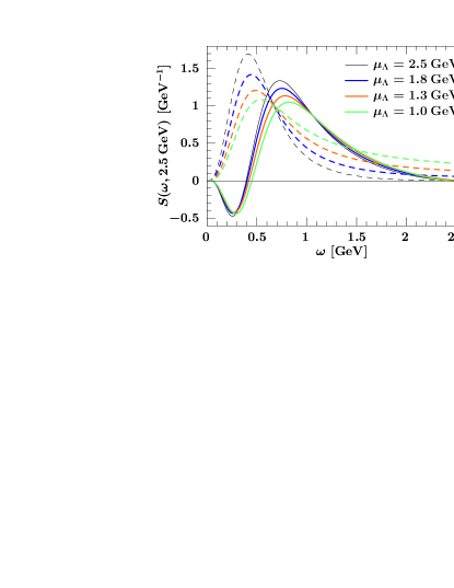
A common approach for modeling a parton distribution function is to specify a model for $S(\omega,\mu_{\Lambda})$ at a fixed scale $\mu_{\Lambda}$ and then run it up to a higher $\mu_{i}$. In this case, $\mu_{\Lambda}$ must be treated as a model parameter, and changing it can cause significant changes in the model. Furthermore, for $\omega\gg\Lambda_{\mathrm{QCD}}$ the perturbative tail of $S(\omega,\mu_{i})$ obtained in this approach will not be consistent with carrying out the OPE at $\mu_{i}$. The perturbative logarithms are reproduced, but the constant terms are not (and the latter are sizeable contributions to the OPE for the scales considered here). In Fig. 1 we compare this approach (dashed curves), with the superior approach of describing the shape function via Eq. (24) (solid curves) at NNLL. In each case we use a model for $F(k)$, $\widehat{F}^{\rm mod}(k)$ given below in Eq. (34), whose first three moments correspond to $m_{b}=4.7\,\mathrm{GeV}$ and $\lambda_{1}=-0.31\,\mathrm{GeV}^{2}$. The thin black dashed curve shows $S(\omega,\mu_{i})=\widehat{F}^{\rm mod}(\omega)$. The other three dashed curves show the result of fixing $S(\omega,\mu_{\Lambda})=\widehat{F}^{\rm mod}(\omega)$ at $\mu_{\Lambda}=1.0,\,1.3,\,1.8\,\mathrm{GeV}$ (from bottom to top near the peaks) and running up to $\mu_{i}=2.5\,\mathrm{GeV}$ using Eq. (1). The resulting tails at large $\omega$ are clearly inconsistent with each other. The solid curves show the result of our approach, using Eq. (24) to obtain $S(\omega,\mu_{\Lambda})$ at $\mu_{\Lambda}=1.0,\,1.3,\,1.8,\,2.5\,\mathrm{GeV}$ and running up to $\mu_{i}=2.5\,\mathrm{GeV}$. In our approach, $S(\omega,\mu_{i})$ is independent of the initial scale $\mu_{\Lambda}$, up to subleading corrections in $\alpha_{s}(\mu_{\Lambda})$, and the tails at large $\omega$ are consistent with one another. The negative dip at small $\omega$ is an artifact of using the pole mass scheme, and will be removed by switching to short distance schemes in the next section. Another feature of the solid curves in Fig. 1 is that their tails become negative for $\omega\gtrsim 2.5\,\mathrm{GeV}$. It was noted in Ref. Bosch:2004th that most of this negative tail is canceled by the perturbative corrections from the jet function. We discuss in Sec. III.3 that this negative tail also disappears if $\mu_{\Lambda}$ is increased as $\omega$ increases.

To obtain the correct perturbative tail, the procedure used by BLNP Lange:2005yw for $|V_{ub}|$ analyses is to take the perturbative computation of $C_{0}(\omega,\mu)$ for $\omega\geq\omega_{0}$ and a model for $S(\omega,\mu)$ for $\omega\leq\omega_{0}$, and these two pieces are glued together, choosing $\omega_{0}$ so that the result is continuous. The advantage of our construction in Eq. (21) is that the tail automatically turns on in a smooth manner when it dominates over the nonperturbative function $F(k)$ and provides the proper $\mu$ dependence for $S(\omega,\mu)$ at any $\omega$.

Imposing the moment constraints on $F(k)$ in Eq. (23) provides a clean way to incorporate the information on the local OPE matrix elements, $m_{b}$, $\lambda_{1}$, etc., from $B\to X_{c}\ell\bar{\nu}$. It is possible to use a shape function scheme in which moments of $S(\omega,\mu)$ with a cutoff define the nonperturbative parameters Bosch:2004th . Our approach has the advantage of allowing one to use any desired short distance scheme, as we discuss next.

III.2 Short distance schemes

The most precise information on the matrix elements in Eq. (16) is provided by fitting OPE results to $B\to X_{c}\ell\bar{\nu}$ decay distributions. This directly constrains $F(k)$ through Eq. (23). Ideally, we would like to incorporate these constraints on $F$ in a manner that is independent of the order in perturbation theory used to calculate $P$ in Eq. (II). However, if we define the moment parameters $\delta$ and $\lambda_{1}$ from Eq. (16) in an infrared sensitive manner such as the pole mass scheme, then the dependence on the order in $\alpha_{s}$ will not be small — infrared renormalon ambiguities in the perturbation series will cancel against ambiguities in the parameters $\delta$ and $\lambda_{1}$. In practice, this means that the values of $\delta$ and $\lambda_{1}$ may change substantially when the fit in $B\to X_{c}\ell\bar{\nu}$ is done at different orders in perturbation theory. In $B$ physics, cancellations between perturbative corrections are significant already at low orders in perturbation theory. Thus, it is preferable to define $F(k)$ and $C_{0}(\omega,\mu)$ so that they are individually free of renormalon ambiguities, which should make the values of $\delta$ and $\lambda_{1}$ more stable to the inclusion of perturbative corrections.

Consider shifting to a new perturbative kernel $\widehat{C}_{0}(\omega,\mu)$ and nonperturbative function $\widehat{F}(k)$ that are free from renormalons. To implement this we let

$$C_{0}(\omega) =\widehat{C}_{0}(\omega)+\delta C_{0}(\omega)\,,$$

$$F(k) =\widehat{F}(k)+\delta F(k)\,,$$ (26)

such that

$$S(\omega)=\int\!\mathrm{d}k\,C_{0}(\omega-k)F(k)=\int\!\mathrm{d}k\,\widehat{C}_{0}(\omega-k)\,\widehat{F}(k)\,.$$ (27)

These shifts move a series of perturbative corrections between $F(k)$ and $C_{0}(\omega,\mu)$. The shift $\delta F(k)$ will be chosen such that the moments of $\widehat{F}(k)$ are given by renormalon-free parameters, and Eq. (27) then determines the corresponding shift $\delta C_{0}(\omega)$.

We switch from the pole mass $m_{b}$ and $\lambda_{1}$ to short distance parameters, $\widehat{m}_{b}$ and $\widehat{\lambda}_{1}$,

$$m_{b}=\widehat{m}_{b}+\delta m_{b}\,,\qquad\lambda_{1}=\widehat{\lambda}_{1}+\delta\lambda_{1}\,,$$ (28)

where $\delta m_{b}$ and $\delta\lambda_{1}$ consist of series in $\alpha_{s}(\mu)$ with the same renormalon as $m_{b}$ and $\lambda_{1}$, respectively. The freedom to choose these series corresponds to the freedom to choose different schemes for $\widehat{m}_{b}$ and $\widehat{\lambda}_{1}$. To obtain $\widehat{F}(k)$ with moments only depending on $\widehat{m}_{b}$ and $\widehat{\lambda}_{1}$, we pick $\delta F(k)$ such that

$$\delta F(k) =F(k)-F(k-\delta m_{b})-\Delta F(k)\,,$$

$$\widehat{F}(k) =F(k-\delta m_{b})+\Delta F(k)\,.$$ (29)

Shifting the argument allows us to switch to $\widehat{m}_{b}$. To implement $\widehat{\lambda}_{1}$, $\Delta F(k)$ has to satisfy

$$\int\!\mathrm{d}k\,\Delta F(k) =\int\!\mathrm{d}k\,k\,\Delta F(k)=0\,,$$

$$\int\!\mathrm{d}k\,k^{2}\,\Delta F(k) =\frac{\delta\lambda_{1}}{3}\,.$$ (30)

The most general solution to Eq. (III.2) is $\Delta F(k)=(\delta\lambda_{1}/6)\,F_{1}^{\prime\prime}(k)$, where $F_{1}(k)$ is an arbitrary function, normalized as $\int\!\mathrm{d}k\,F_{1}(k)=1$.

Using Eqs. (III.2) and (III.2) with Eq. (23), one can easily check that $\widehat{F}(k)$ has renormalon-free moments, as desired,

$$\int\!\mathrm{d}k\,\widehat{F}(k)=1\,,$$

$$\int\!\mathrm{d}k\,k\,\widehat{F}(k)=\delta+\delta m_{b}=\widehat{\delta}\,,$$

$$\int\!\mathrm{d}k\,k^{2}\,\widehat{F}(k)=-\frac{\widehat{\lambda}_{1}}{3}+\widehat{\delta}^{\,2}\,,$$ (31)

where $\widehat{\delta}=m_{B}-\widehat{m}_{b}$. Thus the experimental values of the $b$ quark mass and $\widehat{\lambda}_{1}$ extracted in any short distance scheme can be used as inputs in our framework via the moment constraints in Eq. (III.2).

To determine the corresponding shift in $C_{0}(\omega)$, we note that Eq. (27) implies $\int\!\mathrm{d}k\,[C_{0}(\omega-k)\,\delta F(k)+\delta C_{0}(\omega-k)\,\widehat{F}(k)]=0$. To solve for $\delta C_{0}(\omega)$, we take the Fourier transform, $\delta\widetilde{C}_{0}(y)=-\widetilde{C}_{0}(y)\,\delta\widetilde{F}(y)/\,\widetilde{\!\widehat{F}}(y)$, and thus

$$\delta\widetilde{C}_{0}(y)=\biggl{[}1-e^{iy\,\delta m_{b}}-\frac{\delta\lambda_{1}}{6}\,y^{2}\,\frac{\widetilde{F}_{1}(y)}{\,\widetilde{\!\widehat{F}}(y)}\biggr{]}\widetilde{C}_{0}(y)\,.$$ (32)

Here, any $\delta m_{b}\,\delta\lambda_{1}$ cross terms only have higher-order renormalon ambiguities and are dropped. Any choice of $F_{1}(k)$ is equally good for incorporating the $\delta\lambda_{1}$ shift. We adopt the simplest choice $F_{1}(k)=\widehat{F}(k)$, which is unique in that it keeps $\widehat{C}_{0}(\omega)$ independent of the precise form of $\widehat{F}(k)$. In this case, in momentum space, we have

$$\widehat{C}_{0}(\omega) =C_{0}(\omega+\delta m_{b})-\frac{\delta\lambda_{1}}{6}\,\frac{\mathrm{d}^{2}}{\mathrm{d}\omega^{2}}\,C_{0}(\omega)$$

$$=\biggl{[}1+\delta m_{b}\,\frac{\mathrm{d}}{\mathrm{d}\omega}+\bigg{(}\frac{(\delta m_{b})^{2}}{2}-\frac{\delta\lambda_{1}}{6}\bigg{)}\frac{\mathrm{d}^{2}}{\mathrm{d}\omega^{2}}\biggr{]}C_{0}(\omega)$$

$$\quad+\ldots\,,$$ (33)

where $C_{0}(\omega)$ is determined by the perturbative calculation of $\langle b_{v}\lvert O_{0}(\omega+\delta,\mu)\rvert b_{v}\rangle$, and the ellipsis denotes terms that are either $\mathcal{O}(\alpha_{s}^{3})$ or beyond the order we are working at for the moments of $\widehat{F}(k)$. The same strategy to determine $\widehat{F}(k)$ and derive the corresponding $\widehat{C}_{0}(\omega)$ can be applied to higher moments if in the future terms with $n\geq 3$ in Eq. (23) are included in the analysis.

In the remainder of this paper we use the convolution formula for $S(\omega,\mu)$ in terms of $\widehat{C}_{0}(\omega,\mu)$ and $\widehat{F}(k)$ in Eq. (27). We shall regard $\widehat{F}(k)$ as the fundamental nonperturbative object to be extracted from data. In particular, in Sec. IV we will build a complete basis of functions for $\widehat{F}(k)$.

Parameter	Value
$\alpha_{s}(m_{Z})$ pdg	$0.1176$
$\alpha_{s}(4.7\,\mathrm{GeV})$	$0.2155$
$m_{B}$	$5.279\,\mathrm{GeV}$
$m_{b}^{1S}$ Barberio:2007cr	$4.70\,\mathrm{GeV}$
$\lambda_{1}$ Barberio:2007cr	$-0.31\,\mathrm{GeV}^{2}$
$\lambda_{1}^{\mathrm{i}}$	$-0.32\,\mathrm{GeV}^{2}$
$m_{b}^{\mathrm{kin}}(1\,\mathrm{GeV})$	$4.57\,\mathrm{GeV}$
$\lambda_{1}^{\mathrm{kin}}(1\,\mathrm{GeV})$	$-0.47\,\mathrm{GeV}^{2}$

Table 1: Central values of the input parameters. The last three entries are computed from $m_{b}^{1S}$ and $\lambda_{1}$ at order $\alpha_{s}^{2}$.

III.3 Numerical results for $S(\omega,\mu)$

To illustrate the effect of using our method to include the perturbative corrections to the shape function through $\widehat{C}_{0}$ we choose a model for $\widehat{F}(k)$,

$$\widehat{F}^{\rm mod}(k)=\frac{1}{\lambda}\,\biggl{[}\sum_{n=0}^{2}c_{n}\,f_{n}\Bigl{(}\frac{k}{\lambda}\Bigr{)}\biggr{]}^{2}\,.$$ (34)

Here $\lambda=0.8\,\mathrm{GeV}$, $f_{n}(x)$ is given below in Eq. (48), and the three parameters, $c_{0}$, $c_{1}$, and $c_{2}$, are fixed to satisfy the constraints in Eq. (III.2) for the appropriate short distance scheme. For our numerical analysis we use the input values collected in Table 1. With $\{m_{b}^{1S},\,\lambda_{1}\}$ we have $\{c_{0},\,c_{1},\,c_{2}\}=\{0.949,\,-0.309,\,0.064\}$, while for $\{m_{b}^{1S},\,\lambda_{1}^{\mathrm{i}}\}$ we have $\{c_{0},\,c_{1},\,c_{2}\}=\{0.949,\,-0.307,\,0.075\}$, and for $\{m_{b}^{\rm kin},\,\lambda_{1}\}$ we have $\{c_{0},\,c_{1},\,c_{2}\}=\{0.988,\,-0.120,\,-0.095\}$.

Figure 2: $S(\omega,\mu_{i})$ obtained from $\widehat{C}_{0}(\omega,\mu_{\Lambda})$ with $\mu_{\Lambda}=1.3\,\mathrm{GeV}$ and run up to $\mu_{i}=2.5\,\mathrm{GeV}$ at NLL (dashed) and NNLL (solid) order. Shown are results using the pole mass scheme and the $1S$ and kinetic short distance mass schemes. Switching to the short distance schemes, the result becomes more stable going from NLL to NNLL, the negative dip at small $\omega$ in the pole scheme is removed, while the perturbative tail at large $\omega$ remains unchanged.

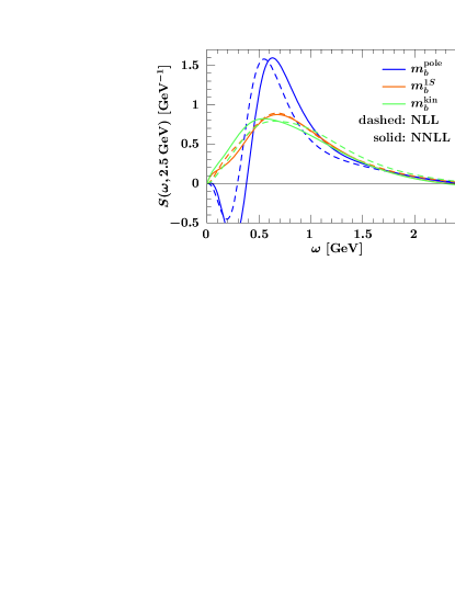
First, we switch from the pole mass to a short distance mass. We use the $1S$ mass Hoang:1998ng and the kinetic mass Czarnecki:1997sz schemes,

$$\widehat{\delta} \equiv\delta^{1S}=m_{B}-m_{b}^{1S}\,,$$

$$\widehat{\delta} \equiv\delta^{\mathrm{kin}}=m_{B}-m_{b}^{\mathrm{kin}}\,,$$ (35)

to fix the first moment in Eq. (III.2), and $\lambda_{1}$ to determine the second moment. The choice of mass scheme enters $\widehat{C}_{0}(\omega)$ through the $\delta m_{b}$ and $\delta\lambda_{1}$ in Eq. (III.2), which must be expanded in $\alpha_{s}$ to avoid the renormalons. Details of the implementation of short distance schemes and the expressions for $\delta m_{b}^{1S}$ and $\delta m_{b}^{\mathrm{kin}}$ are discussed in Appendix A.3. In Fig. 2 we show the result for $S(\omega,\mu_{i})$ obtained from $C_{0}(\omega,\mu_{\Lambda})$ with $\mu_{\Lambda}=1.3\,\mathrm{GeV}$, run up to $\mu_{i}=2.5\,\mathrm{GeV}$ at NLL order (dashed) and NNLL order (solid). The blue (dark), orange (medium), and green (light) curves show the results in the pole, $1S$, and kinetic mass schemes, respectively. In both short distance mass schemes the negative dip present in the pole scheme is removed, while the perturbative tail at large $\omega$ remains unchanged. The removal of the negative dip is similar to what was observed for the soft function for jets in Ref. Hoang:2007vb .

Figure 3: $\mu_{\Lambda}$ dependence of $S(\omega,2.5\,\mathrm{GeV})$ in the peak region obtained from $\widehat{C}_{0}(\omega,\mu_{\Lambda})$ at LL (dotted green), NLL (dashed blue), and NNLL (solid orange) order, using $m_{b}^{1S}$ and $\lambda_{1}$. The three curves in each case are for $\mu_{\Lambda}=1.0,\,1.3,\,1.8\,\mathrm{GeV}$. The $\mu_{\Lambda}$ dependence is significantly reduced at each higher order.

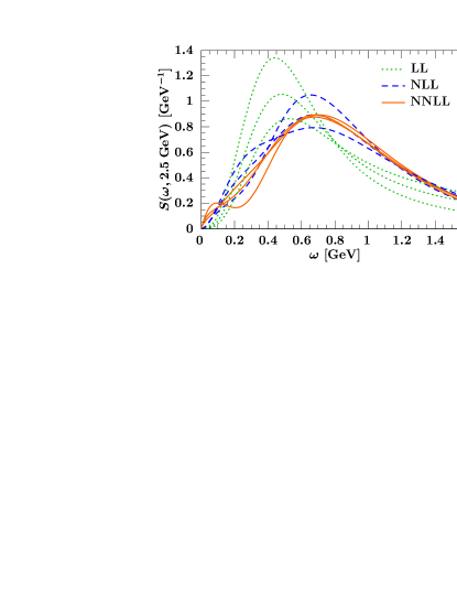
In Fig. 3 we illustrate the perturbative convergence and residual $\mu_{\Lambda}$ scale dependence of the result of Eq. (24) order by order, using the $1S$ mass scheme and $\lambda_{1}$. We show $S(\omega,\mu_{i}=2.5\,\mathrm{GeV})$ run up from $\mu_{\Lambda}$ at LL (dotted green), NLL (dashed blue) and NNLL (solid orange). For each order, the three curves correspond to $\mu_{\Lambda}=1.0,\,1.3,\,1.8\,\mathrm{GeV}$. As expected, the $\mu_{\Lambda}$ dependence is significantly reduced by going from LL to NLL to NNLL. For the lowest scale, $\mu_{\Lambda}=1.0\,{\rm GeV}$, an oscillation begins to build up at small $\omega$, which is clear at NNLL where the curves for the two larger scales are quite stable. Although we continue to explore $\mu_{\Lambda}$ as low as $1.0\,\mathrm{GeV}$ in this section, we take this as evidence that slightly larger values of $\mu_{\Lambda}$ should be used to ensure a convergent expansion for $\widehat{C}_{0}$. Therefore, we will use $\mu_{\Lambda}=1.2,\,1.5,\,1.9\,\,\mathrm{GeV}$ in Sec. III.4 for the decay rate.

Figure 4: The effect of using the invisible scheme for $\lambda_{1}$ on $S(\omega,2.5\,\mathrm{GeV})$ at NNLL order. The orange solid lines are the same as those in Fig. 3, using $m_{b}^{1S}$ and $\lambda_{1}$, while the light blue dashed lines use $m_{b}^{1S}$ together with $\lambda_{1}^{\mathrm{i}}$. The three curves in each case are for the same values of $\mu_{\Lambda}$ as in Fig. 3.

Next, we switch to short distance schemes for $\lambda_{1}$. Note that the NLL results in Fig. 2 with $\lambda_{1}$ defined in dimensional regularization are already quite stable. Unlike for the pole mass, there is not much numerical evidence for the importance of switching to a short distance scheme for $\lambda_{1}$, and adding a sizable $\delta\lambda_{1}\sim{\cal O}(\alpha_{s})$ correction may oversubtract. The $u=1$ renormalon in $\lambda_{1}$ is related to the large-order behavior of perturbation theory, and it is unclear how much numerical impact it has on the perturbative coefficients computed at ${\cal O}(\alpha_{s})$ and ${\cal O}(\alpha_{s}^{2})$. In App. C we show that schemes with $\delta\lambda_{1}={\cal O}(\alpha_{s})$ appear to oversubtract, causing large oscillations in the shape function at small $\omega$. This is shown explicitly for the kinetic scheme $\lambda_{1}^{\rm kin}(=-\mu_{\pi}^{2})$. Therefore, in App. C we introduce a new short distance scheme with $\delta\lambda_{1}=\mathcal{O}(\alpha_{s}^{2})$, which we call the “invisible” scheme and denote by $\lambda_{1}^{\mathrm{i}}$. The expression for $\delta\lambda_{1}^{\mathrm{i}}$ is given in Eq. (101). In this short distance scheme, the NLL results are unchanged. In Fig. 4 we compare results at NNLL for $m_{b}^{1S}$ and $\lambda_{1}$ versus using $m_{b}^{1S}$ and $\lambda_{1}^{\mathrm{i}}$. One sees that the invisible scheme has only a small effect on the NNLL shape function, which is entirely at small $\omega$. It damps the oscillation that occurs when $\mu_{\Lambda}=1.0\,{\rm GeV}$ and modifies the slope.

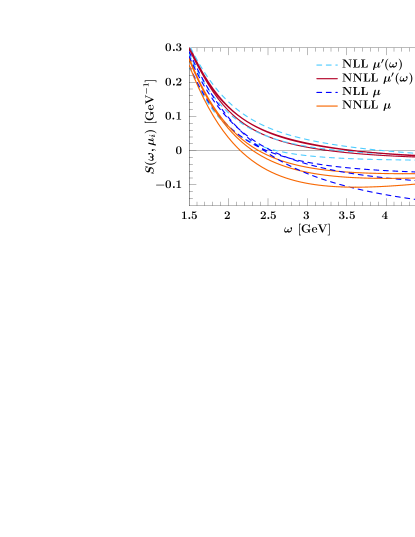
In Fig. 5 we show the $\mu_{\Lambda}$ scale dependence at NLL (dashed) and NNLL (solid) order in the tail region. The lower six curves use the same scale variation as in Fig. 3. Here, as one uses the SCET expansion, but enters the local OPE region, the scale dependence increases with $\omega$, and the tail becomes negative. This is due to increasing $\ln(\omega/\mu_{\Lambda})$ terms, for which the above choices of $\mu_{\Lambda}$ are inappropriate. To avoid potentially large logarithms, we can increase $\mu_{\Lambda}$ as we increase $\omega$ by taking, for example,

$$\mu^{\prime}_{\Lambda}(\omega)=a+b\,\arctan\bigl{(}\omega-2.5\,{\rm GeV}\bigr{)}\,.$$ (36)

To vary the scales, we take three functions of this form, with $a$ and $b$ chosen such that for $\omega=0$ they give $\mu^{\prime}_{\Lambda}=1.0,\,1.3,\,1.8\,\mathrm{GeV}$, and for $\omega=4.7\,\mathrm{GeV}$ they give $\mu^{\prime}_{\Lambda}=2.35,\,4.7,\,9.4\,\mathrm{GeV}$. In Fig. 5, the six upper curves show $S(\omega,\mu_{i})$ obtained with these $\mu^{\prime}_{\Lambda}(\omega)$ choices, taking $\mu_{i}=\mu_{i}^{\prime}(\omega)=[\mu^{\prime}_{\Lambda}(\omega)\,m_{b}^{1S}]^{1/2}$ with the central $\mu^{\prime}_{\Lambda}(\omega)$. Comparing the upper and lower curves shows that increasing $\mu_{\Lambda}$ with $\omega$ significantly reduces the $\mu_{\Lambda}$ scale dependence to a similar level as in the peak region shown in Fig. 3. (We have checked that using the running $\mu_{\Lambda}^{\prime}(\omega)$ does not have an effect on the size of the scale uncertainty in the peak region.) The upper curves in Fig. 5 also have a much less negative tail, which is caused predominantly by increasing $\mu_{\Lambda}$ with $\omega$, and only partially by increasing the reference scale $\mu_{i}$. This means that the dominant part of the negative tail in the lower curves is caused by large logarithms of $\omega/\mu_{\Lambda}$. Hence, increasing $\mu_{\Lambda}$ with $\omega$ will be important to obtain a positive rate in the tail region. The importance of increasing $\mu$ with a kinematic variable in the tail region was also pointed out for jet production in Ref. Fleming:2007xt , where it was required to avoid a negative tail for the cross section.

In the decay rate the $\mu_{i}$ dependence of $S(\omega,\mu_{i})$ cancels against corrections from the jet function, so the intermediate scale, $\mu_{i}$, should also run with increasing $\omega$. This is accomplished by taking $\mu_{i}=\mu_{i}^{\prime}(\omega)=[\mu^{\prime}_{\Lambda}(\omega)\,\mu_{b}]^{1/2}$ for each of the three running $\mu_{\Lambda}^{\prime}(\omega)$’s from Eq. (36). This treatment of the tail has the advantage that we obtain $\mu_{\Lambda}=\mu_{i}=\mu_{b}$ for $\omega\sim m_{b}$, and by construction the standard factor of two scale variation, $m_{b}/2<\mu_{b}<2m_{b}$. Hence it is consistent with the local OPE treatment for region 3) in Eq. (II). The rate at which equality is approached can be controlled by multiplying the argument of the $\arctan$ in Eq. (36) by a scaling factor, and the center of the transition region can be adjusted by modifying the $2.5\,{\rm GeV}$ value shown there.

Figure 5: $\mu_{\Lambda}$ dependence of $S(\omega,2.5\,\mathrm{GeV})$ in the tail region (lower six curves) and of $S(\omega,\mu_{i}^{\prime})$ (upper six curves) at NLL (dashed) and NNLL (solid) order, using $m_{b}^{1S}$ and $\lambda_{1}^{\mathrm{i}}$. For the lower six curves we vary $\mu_{\Lambda}=1.0,\,1.3,\,1.8\,\mathrm{GeV}$, while for the upper ones we use the running scale parameters $\mu^{\prime}_{\Lambda}(\omega)$ in Eq. (36) and $\mu^{\prime}_{i}(\omega)$ described in the text.

III.4 Perturbative results for the $B\to X_{s}\gamma$ spectrum

In this section we explore the scale dependence of the perturbative corrections to the $B\to X_{s}\gamma$ spectrum in the SCET regions 1) and 2) in Eq. (II). The rate depends on three scale parameters $\mu_{\Lambda}\gtrsim 1\,\mathrm{GeV}$, $\mu_{i}\sim\sqrt{m_{b}\,\Lambda_{\rm QCD}}$, and $\mu_{b}\sim m_{b}$. In a short distance scheme the decay rate in Eq. (II) becomes

$$\frac{\mathrm{d}\Gamma_{s}}{\mathrm{d}p_{X}^{+}} =\Gamma_{0s}\,H_{s}(p_{X}^{+},\mu_{b})\,U_{H}(m_{b},\mu_{b},\mu_{i})$$

$$\quad\times\int\!\mathrm{d}k\,\widehat{P}(m_{b},k,\mu_{i})\,\widehat{F}(p_{X}^{+}-k)\,,$$ (37)

where $H_{s}$ and $U_{H}$, are given in Eqs. (A.1) and (78), and the notation $\widehat{P}$ and $\widehat{F}$ indicate that these are given in a short distance scheme. From the analysis in App. A, all perturbative corrections can be organized into a simple series of plus distributions $\mathcal{L}_{j}^{\eta}(z)$, defined in Eqs. (111) and (112). The integral of the perturbative function $P$ with the $F$ function is then

$$\int\!\mathrm{d}k\,P(p^{-},k,\mu_{i})\,F(p_{X}^{+}-k)$$ (38)

$$\quad=\sum_{j=-1}^{\infty}P_{j}(p^{-},p_{X}^{+},\mu_{i},\mu_{\Lambda})\int_{0}^{1}\!\mathrm{d}z\,\mathcal{L}_{j}^{\eta}(z)\,F[p_{X}^{+}(1-z)]\,,$$

where explicit results for the coefficients $P_{j}$ are given in Eq. (A.2). The additional terms generated by transforming Eq. (38) into the integral over the short distance $\widehat{P}$ and $\widehat{F}$ are described in detail in App. A.3.

Figure 6: $\mu_{\Lambda}$ dependence of the $B\to X_{s}\gamma$ spectrum in terms of $m_{b}^{1S}$ and $\lambda_{1}^{\mathrm{i}}$, using $\widehat{F}^{\rm mod}(k)$. Shown are the LL (dotted), NLL (dashed), and NNLL (solid) spectra for $\mu_{\Lambda}=1.2,\,1.5,\,1.9\,\mathrm{GeV}$. The long dashed curves are the NNLL spectra with $m_{b}^{1S}$ and $\lambda_{1}$, showing less convergence at small $\omega$.

Figure 7: $\mu_{i}$ dependence of the $B\to X_{s}\gamma$ spectrum in terms of $m_{b}^{1S}$ and $\lambda_{1}^{\mathrm{i}}$, using $\widehat{F}^{\rm mod}(k)$, at LL (dotted), NLL (dashed), and NNLL (solid) order for $\mu_{i}=2.0,\,2.5,\,3.0\,\mathrm{GeV}$.

Figure 8: $\mu_{b}$ dependence of the $B\to X_{s}\gamma$ spectrum in terms of $m_{b}^{1S}$ and $\lambda_{1}^{\mathrm{i}}$, using $\widehat{F}^{\rm mod}(k)$, at LL (dotted), NLL (dashed), and NNLL (solid) order for $\mu_{b}=2.35,\,4.7,\,9.4\,\mathrm{GeV}$.

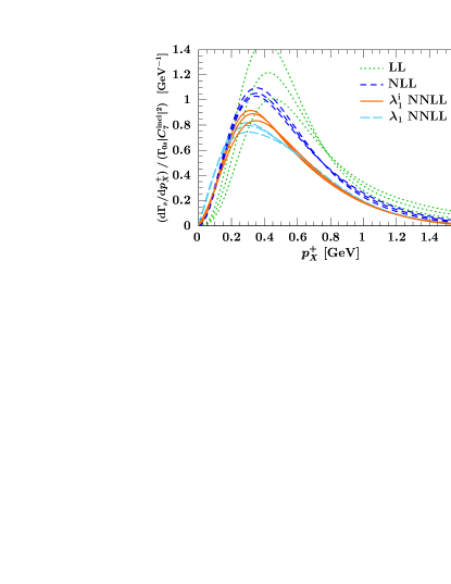
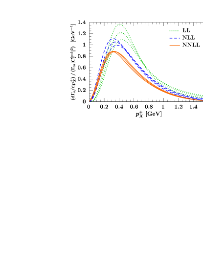
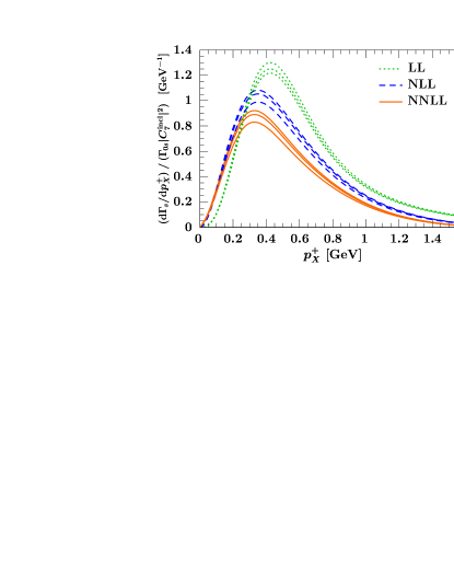
In Figs. 8, 8, and 8 we study the $\mu_{\Lambda}$, $\mu_{i}$, and $\mu_{b}$ dependencies of the $p_{X}^{+}$ spectrum for $B\to X_{s}\gamma$, namely $(\mathrm{d}\Gamma_{s}/\mathrm{d}p_{X}^{+})/\bigl{[}\Gamma_{0s}\,|C_{7}^{\rm incl}(0)|^{2}\bigr{]}$. Recall that this has a simple relation to the photon energy spectrum, $p_{X}^{+}=m_{B}-2E_{\gamma}$. We show the $p_{X}^{+}$ spectrum to facilitate easier comparison with the results for the shape function in the previous section. Since we are interested in studying the perturbative corrections, we keep $\widehat{F}^{\rm mod}(k)$ fixed to be our default model in Eq. (34). In each of Figs. 8, 8, and 8 we show results at LL (dotted green curves), NLL (dashed blue curves), and NNLL (solid orange curves) order, for three different values of the scales, and using the $1S$ mass and $\lambda_{1}^{\mathrm{i}}$ scheme. The central values are $\mu_{\Lambda}=1.5\,\mathrm{GeV}$, $\mu_{i}=2.5\,\mathrm{GeV}$, and $\mu_{b}=4.7\,\mathrm{GeV}$, two of which are held fixed in each plot. In Fig. 8 the three curves at each order show $\mu_{\Lambda}=1.2,\,1.5,\,1.9\,\mathrm{GeV}$, in Fig. 8 they show $\mu_{i}=2.0,\,2.5,\,3.0\,\mathrm{GeV}$, and in Fig. 8 they show $\mu_{b}=2.35,\,4.7,\,9.4\,\mathrm{GeV}$. Since the scales should obey the hierarchy $\mu_{\Lambda}<\mu_{i}<\mu_{b}$, it is not possible to vary each by a factor of two. For illustration, we do vary $\mu_{b}$ by a factor of two, but keep $\mu_{\Lambda}$ and $\mu_{i}$ in ranges suitable to the physical shape function and jet function regions, respectively. The largest effect going from LL to NLL to NNLL is the change in the normalization. Although it is not captured by our range of scale variation, the normalization still exhibits reasonable convergence. Rescaled to a common normalization, the shape of the spectrum shows very nice convergence, and the range of scales used is clearly suitable here. We find a reduction in the scale dependence order by order for most values of $p_{X}^{+}$.

In Fig. 8 we show three additional NNLL curves (long dashed light blue) that use $m_{b}^{1S}$ and $\lambda_{1}$ instead of $\lambda_{1}^{\mathrm{i}}$. Comparing these curves to the orange curves ($m_{b}^{1S}$ and $\lambda_{1}^{\mathrm{i}}$), we see that the overall effect of using $\lambda_{1}^{\mathrm{i}}$ instead of $\lambda_{1}$ is small. However, one can clearly observe that the invisible scheme improves the perturbative convergence of the spectrum at small $p_{X}^{+}$.

Although we do not show results here for the spectrum in the local OPE region 3) in Eq. (II), we checked that the same effects as in the tail of $S(\omega,\mu_{i})$ in Fig. 5 appear in the tail of the spectrum. To avoid a large $\mu_{\Lambda}$ dependence in the tail, the scales must be increased with $\omega$ as discussed below Eq. (36), and this also helps to obtain a positive tail for the spectrum in region 3).

It is important to emphasize that in the common approach to model distribution functions corresponding to the dashed curves in Fig. 1, where a fixed model for $S(\omega,\mu_{\Lambda})$ is specified at the scale $\mu_{\Lambda}$ and then run up to $\mu_{i}$, the spectrum will have a large dependence on $\mu_{\Lambda}$, which must be considered a model parameter. Thus, there is no analog to the $\mu_{\Lambda}$ independence of the rate obtained in our construction, and illustrated in Fig. 8. Note that the dependence of the $B\to X_{s}\gamma$ rate for $p_{X}^{+}\leq(p_{X}^{+})^{\mathrm{cut}}$ on the soft and intermediate scales, $\mu_{\Lambda}$ and $\mu_{i}$, has so far been studied only by performing an expansion in $\Lambda_{\mathrm{QCD}}/(p_{X}^{+})^{\mathrm{cut}}$ in region 2) of Eq. (II) Neubert:2004dd ; Becher:2006pu , as in Eqs. (III.1) and (14). In this case, one can combine the same perturbative ingredients as in our approach, depending on the three scales $\mu_{\Lambda}$, $\mu_{i}$, and $\mu_{b}$. As mentioned before, the advantage of our framework is that it does not rely on performing an expansion in region 2).

IV Expansion of the $F$ Function

IV.1 Complete orthonormal basis

So far in the literature the uncertainty related to the unknown functional form of the shape function has been either neglected or estimated by using a few model functions for $S(\omega,\mu)$, and varying their parameters or distorting them Lee:2005pw ; Lange:2005yw ; DeFazio:1999sv ; Gambino:2007rp , subject to constraints on their first few moments. To obtain a systematic estimate of the uncertainty related to the unknown functional form of the shape function, we construct a suitable set of complete orthonormal basis functions for the function $\widehat{F}(k)$ defined by Eq. (27). The uncertainty in the functional form is then determined by the uncertainty in the coefficients of this basis. This expansion will also be convenient to extract $\widehat{F}(k)$ from experimental data, including experimental and theoretical uncertainties and correlations.

Since $\widehat{F}(k)$ has mass dimension $-1$, it is convenient to introduce a dimension-one parameter, $\lambda$, and use the dimensionless variable $x=k/\lambda$. By power counting, $\lambda\sim\Lambda_{\mathrm{QCD}}$. We expect on physical grounds that $\widehat{F}(k)$ is positive, so we can expand its square root,

$$\widehat{F}(\lambda\,x)=\frac{1}{\lambda}\,\biggl{[}\sum_{n=0}^{\infty}c_{n}\,f_{n}(x)\biggr{]}^{2}\,,$$ (39)

where $f_{n}(x)$ are a complete set of orthonormal functions,

$$\int_{0}^{\infty}\mathrm{d}x\,f_{m}(x)\,f_{n}(x)=\delta_{mn}\,.$$ (40)

Since $\widehat{F}(k)$ is normalized to unity, the coefficients $c_{n}$ satisfy

$$1=\int\!\mathrm{d}k\,\widehat{F}(k)=\int\!\mathrm{d}x\,\biggl{[}\sum_{n}c_{n}\,f_{n}(x)\biggr{]}^{2}=\sum_{n}c_{n}^{2}\,.$$ (41)

Although $\widehat{F}(k)$ is independent of the choice of basis functions $f_{n}(x)$ when summing over all $n$, in practice only a finite number of terms can be kept. Therefore, we want to choose basis functions, $f_{n}(x)$, such that the first few terms in Eq. (39) provide a good approximation to $\widehat{F}(k)$. Unfortunately, most of the well-known orthonormal functions on $[0,\infty)$ become broader with increasing $n$, and hence have moments whose values increase with $n$ book . By dimensional analysis, the $n$-th moment of $\widehat{F}(k)$ scales as $\Lambda_{\mathrm{QCD}}^{n}$, and we would like the basis functions to satisfy this constraint, at least for the low-$n$ moments.

To construct a suitable orthonormal basis $f_{n}(x)$ on $[0,\infty)$, we consider orthonormal functions $\phi(y)$ on $[-1,1]$ and a variable transformation $y(x)$, which maps $x\in[0,\infty)$ to $y\in[-1,1]$. We choose $y(x)$ to be increasing, $y^{\prime}(x)>0$. Then, for any orthonormal basis $\phi_{n}(y)$ on $[-1,1]$,

$$f_{n}(x)=\sqrt{y^{\prime}(x)}\;\phi_{n}[y(x)]\,.$$ (42)

provides an orthonormal basis on $x\in[0,\infty)$. Choosing different $\phi_{n}$’s and different $y(x)$’s allows us to change the basis functions. It is natural to choose $\phi_{n}(y)$ to be polynomials of degree $n$, and we find it convenient to use the normalized Legendre polynomials

$$\phi_{n}(y)=\sqrt{\frac{2n+1}{2}}\,P_{n}(y)\,,\quad P_{n}(y)=\frac{1}{2^{n}n!}\,\frac{\mathrm{d}^{n}}{\mathrm{d}y^{n}}(y^{2}-1)^{n}.$$ (43)

To determine $y(x)$, note that for a positive definite function $Y(x)$, such that $\int_{0}^{\infty}\!\mathrm{d}x\,Y(x)=1$, the function

$$y(x)=-1+2\int_{0}^{x}\!\mathrm{d}x^{\prime}\,Y(x^{\prime})\,,$$ (44)

satisfies $y(0)=-1$ and $y(\infty)=+1$. Since $y^{\prime}(x)=2Y(x)$, the first basis function is simply

$$[f_{0}(x)]^{2}=y^{\prime}(x)\,\phi_{0}^{2}[y(x)]=Y(x)\,.$$ (45)

To obtain a good approximation to $\widehat{F}(k)$ with the first few terms in Eq. (39), one should choose $Y(x)$ to be “similar” to $\lambda\,\widehat{F}(\lambda x)$. This gives an intuition about suitable choices, and once $Y(x)$ and $\lambda$ are fixed, the full basis is specified. A convenient choice for $Y(x)$ is

$$Y(x,p)=\frac{(p+1)^{p+1}}{\Gamma(p+1)}\,x^{p}\,e^{-(p+1)x}\,$$ (46)

for any $p>0$ real parameter. Constructing a basis from $Y(x,p)$ yields basis functions for which the first and second moments of $f_{m}(x)f_{n}(x)$ are order one or smaller. Therefore, the terms in the expansion in Eq. (39) have $n$-th moments of order $\lambda^{n}$ or smaller. Choosing the scaling parameter $\lambda\sim\Lambda_{\mathrm{QCD}}$, the first few terms in the expansion in the resulting basis gives a good approximation to the shape function.

The function in Eq. (46) is similar to those used to model $S(\omega,\mu)$ in the literature. In fact, by choosing $Y(x)$ to be a specific model shape function, our construction allows one to expand about it, and systematically study corrections to an assumed functional form. We emphasize, however, that in our approach the only role of $\phi_{n}(y)$ and $Y(x)$ is to specify the basis functions, $f_{n}(x)$. The functional form for $Y(x)$ affects how quickly the expansion in Eq. (39) converges, but not the fact that it is a convergent expansion. The completeness of the basis $\phi_{n}(y)$ on $[-1,1]$ implies that any square integrable function on $[0,\infty)$ can be expanded in terms of the bases $f_{n}(x)$ resulting from the above construction.

Using Eq. (46) gives basis functions that behave as $f_{n}^{2}(x)\sim x^{p}$ as $x\to 0$. Due to the short distance subtractions in Eq. (III.2), to ensure that $S(\omega,\mu)$ goes to zero at $\omega=0$, we need $\widehat{F}(k)$ to go to zero at least as $k^{3}$ for $k\to 0$. Thus, we find it convenient to use $Y(x,3)$ as our default choice, with

$$y(x,3)=1-2\bigg{(}1+4x+8x^{2}+\frac{32}{3}x^{3}\bigg{)}\,e^{-4x}\,,$$ (47)

which gives the orthonormal functions

$$f_{n}(x)=8\,\sqrt{\frac{2x^{3}\,(2n+1)}{3}}\,e^{-2x}\,P_{n}[y(x,3)]\,.$$ (48)

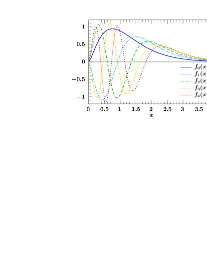
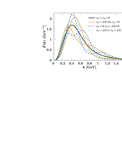
For numerical calculations we use $\lambda=0.8\,\mathrm{GeV}$ as default. These functions are also convenient because they allow analytic calculations of the decay spectra. The first five basis functions in Eq. (48) are shown in Fig. 9. In Fig. 10 we use these to illustrate the uncertainty remaining in $\widehat{F}(k)$ if its first three moments are fixed. We fix $c_{3}$ and $c_{4}$ to 9 different combinations, and choose the first three coefficients $c_{0,1,2}$ to satisfy the moment constraints in Eq. (III.2). All the 9 functions shown have $0.92<c_{0}<0.95$, $-0.35<c_{1}<-0.28$, and $0.01<c_{2}<0.14$. Even this plot makes the uncertainties look smaller than they are, since at small $k$ the $k^{3}$ behavior of these models appears to imply a small uncertainty. Including the short distance subtractions from Eq. (III.2), these models yield a significantly wider variation in $S(\omega,\mu)$ for small $\omega$. Figure 10 shows that even with small errors of the $B\to X_{c}\ell\bar{\nu}$ moments, more information on the shape function can be extracted from the $B\to X_{s}\gamma$ or $B\to X_{u}\ell\bar{\nu}$ data.

Figure 9: The first 5 orthonormal basis functions in Eq. (48).

Figure 10: Nine functions with identical first three moments. For each curve, we fix $c_{3}$ and $c_{4}$ and then choose $c_{0}$, $c_{1}$, $c_{2}$ to satisfy the moment constraints in Eq. (III.2) with $m_{b}^{1S}$ and $\lambda_{1}^{\mathrm{i}}$. The thick solid curve ($c_{3}=c_{4}=0$) corresponds to the default model used in Sec. III.

IV.2 Truncation uncertainties

Figure 11: Left: Expansion of a Gaussian model function $\widehat{F}^{\mathrm{Gauss}}(k)=(2/a)(k/a)^{3}\exp[-(k/a)^{2}]$ with $a=0.639\,\mathrm{GeV}$, corresponding to $m_{b}=4.7\,\mathrm{GeV}$, using the first 5 basis functions, $f_{n}(x)$, in Eq. (48). Right: Same as on the left, except that in the definition of the basis $\lambda$ is changed from $0.8\,\mathrm{GeV}$ to $0.6\,\mathrm{GeV}$.

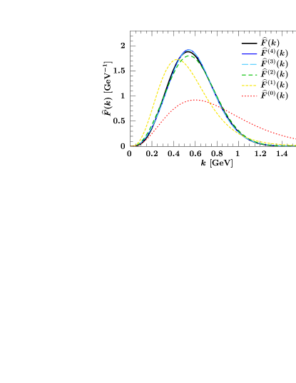
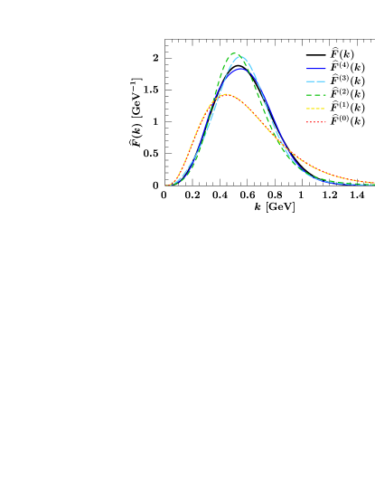
Equation (39) provides a model independent description of $\widehat{F}(k)$ for any choice of the basis. Since the basis is complete for any value of $\lambda$, we will regard $\lambda$ along with the function $Y(x)$ as part of the convention that defines the basis. In practical applications one has to truncate the series in Eq. (39) after the first $N+1$ terms,

$$\widehat{F}^{(N)}(k) \equiv\frac{1}{\lambda}\,\bigg{[}f^{(N)}\Big{(}\frac{k}{\lambda}\Big{)}\bigg{]}^{2}=\frac{1}{\lambda}\,\biggl{[}\sum_{n=0}^{N}c_{n}\,f_{n}\Bigl{(}\frac{k}{\lambda}\Bigr{)}\biggr{]}^{2}$$

$$=\frac{1}{\lambda}\,\sum_{m,n=0}^{N}c_{m}c_{n}\,f_{m}\Bigl{(}\frac{k}{\lambda}\Bigr{)}\,f_{n}\Bigl{(}\frac{k}{\lambda}\Bigr{)}\,,$$ (49)

and use $\widehat{F}^{(N)}(k)$ in the actual calculations.

Figure 11 illustrates how the expansion converges. Both plots show a toy Gaussian model function (black solid curve), which we expand in terms of the first $n$ basis functions in Eq. (48) for $n\leq 4$. In the left panel, we use the default value $\lambda=0.8\,\mathrm{GeV}$ to define the basis. The truncated series in Eq. (IV.2) quickly approaches the model function, even for small values of $N$. In the right panel, we show the same expansion using $\lambda=0.6\,\mathrm{GeV}$ to define the basis, which illustrates how the value of $\lambda$ affects the convergence of the expansion.

To quantify the uncertainties, we would like to have a systematic way to estimate the error due to the neglected terms in the truncated sum in Eq. (IV.2). The truncation error is affected by the choice of $N$, $Y(x)$, and $\lambda$, providing several handles on this uncertainty. A virtue of adding one more term from our orthonormal basis, compared to adding one more parameter to a generic model, is that due to the orthogonality of the basis functions the additional parameter provides independent information and should avoid large parameter correlations. By varying $N$, one can change the number of coefficients, and study how sensitive the results are to the truncation. As a consistency check, one can use a different basis, or change $Y(x)$ or $\lambda$ and check that the difference is within the previous truncation error estimate.

A feature of our construction is that the truncation error can be estimated using $\sum_{n=0}^{\infty}c_{n}^{2}=1$. We define

$$\sqrt{\lambda\,\widehat{F}(\lambda\,x)}\equiv f(x) =f^{(N)}(x)+c_{r}\,f_{r}(x)\,,$$ (50)

where

$$c_{r}=\biggl{(}1-\sum_{n=0}^{N}c_{n}^{2}\biggr{)}^{1/2}\,,$$ (51)

and the remainder function, $f_{r}(x)$, is orthogonal to $f_{0,\ldots,N}(x)$,

$$f_{r}(x)=\sum_{n=1}^{\infty}r_{n}\,f_{N+n}(x)\,,$$ (52)

and normalized

$$\int_{0}^{\infty}\mathrm{d}x\,[f_{r}(x)]^{2}=1\,,\qquad\sum_{n=1}^{\infty}r_{n}^{2}=1\,.$$ (53)

In terms of $f_{r}(x)$, the truncation error from approximating $\widehat{F}(k)$ by $\widehat{F}^{(N)}(k)$ is

$$\widehat{F}^{(N)}_{\mathrm{trunc}}[f_{r}](k) \equiv\bigl{\lvert}\widehat{F}(k)-\widehat{F}^{(N)}(k)\bigr{\rvert}$$ (54)

$$=\frac{1}{\lambda}\,\biggl{\lvert}\,2\,c_{r}f_{r}\Bigl{(}\frac{k}{\lambda}\Bigr{)}\,f^{(N)}\Bigl{(}\frac{k}{\lambda}\Bigr{)}+c_{r}^{2}f_{r}^{2}\Bigl{(}\frac{k}{\lambda}\Bigr{)}\biggr{\rvert}\,.$$

Figure 12: Truncation error estimates. The solid black curves show $\widehat{F}^{\mathrm{Gauss}}(k)-\widehat{F}^{(N)}(k)$ corresponding to the right plot in Fig. 11, for $N=2$ (left) and $N=4$ (right). The dashed blue curves show $\pm\max\big{\{}\widehat{F}^{(N)}_{\mathrm{trunc}}[\pm f_{N+1}]\big{\}}$, and the solid orange curves show $\pm\max\big{\{}\widehat{F}^{(N)}_{\mathrm{trunc}}[\pm f_{0}]\big{\}}$, i.e., the error estimates using Eqs. (55) and (56), respectively.

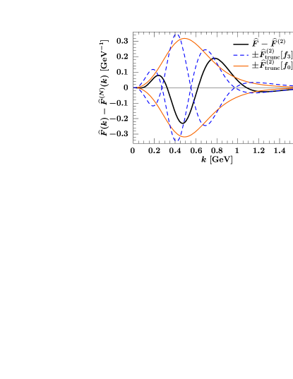
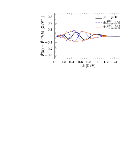
Although Eq. (53) implies $\lvert r_{n}\rvert\leq 1$, it provides no bound on $\sum_{n}\lvert r_{n}\rvert$. Therefore, one cannot derive a rigorous bound on $\lvert f_{r}(x)\rvert$ from Eq. (52) for all $x>0$, and it is not possible to obtain a rigorous bound on the truncation error, $\widehat{F}^{(N)}_{\mathrm{trunc}}$, either. However, for practical purposes, it is sufficient to estimate $\widehat{F}^{(N)}_{\mathrm{trunc}}$. Its size is controlled by $c_{r}$ in Eq. (51), which is determined by the first $N+1$ coefficients, and can be minimized by choosing a good basis. Thus, as long as enough coefficients are included in the basis so that the estimated truncation uncertainty is small compared to other uncertainties, any reasonable estimate of $f_{r}(x)$ provides a useful estimate of the truncation uncertainty.

For suitable choices of the basis, we expect the series to converge fairly quickly, since the higher basis functions oscillate more and more rapidly, and we do not expect significant structure in the momentum distribution of the $b$ quark in the $B$ meson over momentum scales $\ll\Lambda_{\mathrm{QCD}}$. Hence, one way to estimate $f_{r}(x)$ is to assume that one term in Eq. (52) saturates the sum. It is natural to take that to be the first (possibly the second) term, which corresponds to

$$f_{r}(x)=\pm f_{N+1}(x)\,.$$ (55)

Another possibility is to assume that $\lvert f_{r}(x)\rvert\lesssim f_{0}(x)$, and take

$$f_{r}(x)=\pm f_{0}(x)\,.$$ (56)

This is motivated by the fact that, except for small and large values of $x$, $f_{0}(x)$ gives roughly an envelope for the higher basis functions, as can be seen from Fig. 9. In each case, the sign of $f_{r}(x)$ is undetermined. For small $c_{r}$, the second term in Eq. (54) can be neglected and the sign of $f_{r}(x)$ is irrelevant.

To illustrate these methods for estimating the truncation error we consider again the toy model used in Fig. 11, with $\lambda=0.6$ in our basis as in the right panel. In Fig. 12, the solid black curve shows $\widehat{F}(k)-\widehat{F}^{(N)}(k)$ for $N=2$ (left panel) and $N=4$ (right panel). The dashed blue curves show the estimate using Eq. (55), taking the point-by-point maximum of $\widehat{F}^{(N)}_{\mathrm{trunc}}[\pm f_{N+1}](k)$, while the solid orange curves use Eq. (56) instead. As expected, the former correlates more with the absolute value of the point-by-point deviations, while the latter roughly envelopes the difference. As can be seen, we obtain reasonable estimates of the deviation of $\widehat{F}^{(N)}(k)$ from $\widehat{F}(k)$. The overall sizes of the truncation errors are well estimated in both plots, because they are proportional to $c_{r}$. For the left plot $c_{r}=0.088$ and for the right plot $c_{r}=0.025$. If the expansion of $\widehat{F}(k)$ converges reasonably fast, then $f_{r}(x)$ will be an oscillatory function, as shown in Fig. 12. Ultimately we are interested in how the shape function impacts the uncertainty in the extraction of $\lvert V_{ub}\rvert$ or that in determining the $B\to X_{s}\gamma$ event fraction above a certain photon energy cut. These depend on weighted integrals of $\widehat{F}(k)$, so their uncertainties will be much smaller than the point-by-point errors in approximating $\widehat{F}(x)$ by $\widehat{F}^{(N)}(x)$ shown in Fig. 12.

IV.3 Subleading shape functions

Any precision analysis of differential spectra in $B\to X_{s}\gamma$ or $B\to X_{u}\ell\bar{\nu}$ must incorporate power corrections that go beyond Eq. (4). At order $\Lambda_{\mathrm{QCD}}/m_{b}$, six subleading shape functions enter the description of the most general inclusive spectra in $B\to X_{s}\gamma$ and $B\to X_{u}\ell\bar{\nu}$ Bauer:2001mh ; Leibovich:2002ys ; Bauer:2002yu ; Lee:2004ja . We refer to these as the primary subleading shape functions. In addition there are terms in $B\to X_{s}\gamma$ that enter from operators other than $O_{7}$ and are related to the photon’s hadronic structure, whose contribution to the total rate is not calculable in the OPE Kapustin:1995fk ; Lee:2006wn . Considering only the primary subleading shape functions and using suitably weighted integrals of the $B\to X_{u}\ell\bar{\nu}$ differential rate together with $B\to X_{s}\gamma$, the ${\cal O}(\Lambda_{\mathrm{QCD}}/m_{b})$ shape functions can be canceled in the determination of $|V_{ub}|$ Lee:2008vs . However the same drawbacks apply to the weighting method at subleading order as those mentioned already in the introduction, so it is interesting to consider how our analysis can be extended to include these subleading shape functions.

The appropriate factorization theorem for the primary subleading shape functions, analogous to Eq. (4), is known from Ref. Lee:2004ja . Thus, when one-loop partonic calculations of these functions and their corresponding jet functions are available, a construction analogous to Eq. (21) can be carried out to build in the proper large-$\omega$ tail, $\mu_{\Lambda}$ dependence, etc. However, it should be cautioned that a large number of additional shape functions enter in the matching at $\mathcal{O}(\alpha_{s}\Lambda_{\mathrm{QCD}}/m_{b})$ Lee:2004ja ; Beneke:2004in ; Trott:2005vw , so the utility of extending our full analysis to this level is unclear.

Here, we simply discuss how a complete basis can be constructed for the primary subleading shape functions. We know less about these shape functions than about the leading order one. Their moments are still related to HQET matrix elements. In particular, the zeroth moment of the $\mathcal{O}(\Lambda_{\mathrm{QCD}}/m_{b})$ shape functions vanishes, which means they must be negative for some values of $k$, and their first moments either vanish or are given by linear combinations of $\lambda_{1}$ and $\lambda_{2}$. The zeroth moments no longer vanish for the $\mathcal{O}(\Lambda_{\mathrm{QCD}}^{2}/m_{b}^{2})$ shape functions and beyond Leibovich:2002ys, , Mannel:2004as, , Tackmann:2005ub, .

For simplicity, we define the sign of each $\mathcal{O}(\Lambda_{\mathrm{QCD}}/m_{b})$ shape function such that its first nonzero moment is positive. A convenient expansion for the functions with vanishing first moment is given by

$$H(\lambda\,x)=-\frac{\mathrm{d}}{\mathrm{d}x}\,\biggl{[}\sum_{n}d_{n}\,f_{n}(x)\biggr{]}^{2}\,,$$ (57)

while the four-quark operator shape functions, whose zeroth and first moments vanish, can be expanded as

$$H^{4q}(\lambda\,x)=\frac{\mathrm{d}^{2}}{\mathrm{d}x^{2}}\,\biggl{[}\sum_{n}d_{n}\,f_{n}(x)\biggr{]}^{2}\,.$$ (58)

With this form, $\int_{0}^{\infty}\mathrm{d}k\,H^{(4q)}(k)=\int_{0}^{\infty}\mathrm{d}k\,k\,H^{4q}(k)=0$. The first nonzero moments provide constraints on the coefficients, similar to Eq. (41), for example

$$\int_{0}^{\infty}\!\mathrm{d}k\,k\,H(k)=\lambda^{2}\sum_{n}d_{n}^{2}\,,$$ (59)

which can be set to the appropriate linear combinations of $\lambda_{1}$ and $\lambda_{2}$. Note that a different set of coefficients, $d_{n}$, occurs for each subleading shape function.

V Extracting the $F$ Function and predicting decay rates

For a given basis for the leading and subleading shape functions we want to extract the basis coefficients, $c_{i}$ and $d_{i}$, including their uncertainties and correlations. This extraction will use data on the $B\to X_{s}\gamma$ and $B\to X_{u}\ell\bar{\nu}$ spectra and data that determines moments of the shape functions from $B\to X_{c}\ell\bar{\nu}$. To simplify our discussion, we adopt a notation that is suitable for the coefficients $\{c_{0},\ldots,c_{N}\}$ of the function $\widehat{F}(k)$ appearing in the leading shape function. The generalization to incorporate subleading shape functions is straightforward. All results in this section are exact for $N\to\infty$ and for finite $N$ one has to take into account the truncation error discussed in Sec. IV.2.

Since the function $\widehat{F}(k)$ enters the decay spectra linearly, we can independently compute the contributions of the product of any two basis functions, $f_{m}(x)f_{n}(x)$, in the expansion of $\widehat{F}(k)$, which we denote by $\mathrm{d}\Gamma_{mn}$. The differential spectra $\mathrm{d}\Gamma_{s}=\mathrm{d}\Gamma_{s}/\mathrm{d}E_{\gamma}$ or $\mathrm{d}\Gamma_{u}=\mathrm{d}\Gamma_{u}/\mathrm{d}E_{\ell}\mathrm{d}p_{X}^{+}\mathrm{d}p_{X}^{-}$ are then given by

$$\mathrm{d}\Gamma=\sum_{m,n=0}^{N}c_{m}\,c_{n}\,\mathrm{d}\Gamma_{mn}\,,$$ (60)

where from combining Eq. (II) and (39), the $\mathrm{d}\Gamma_{mn}$ are

$$\mathrm{d}\Gamma_{mn} =\Gamma_{0}\,H(p^{-})\!\int_{0}^{p_{X}^{+}}\!\mathrm{d}k\ \frac{\widehat{P}(p^{-},k)}{\lambda}$$

$$\quad\times f_{m}\Bigl{(}\frac{p_{X}^{+}\!-\!k}{\lambda}\Bigr{)}\,f_{n}\Bigl{(}\frac{p_{X}^{+}\!-\!k}{\lambda}\Bigr{)}.$$ (61)

For simplicity, we suppress the scale $\mu$ in the arguments of $H$ and $\widehat{P}$, and the $u$ or $s$ subscripts on $H$. The $\mathrm{d}\Gamma_{mn}$ in Eq. (V) act as a basis for the physically measurable distributions, and the result in Eq. (60) is a quadratic polynomial in each of the fit parameters, $c_{i}$.

In practice, experimental spectra are binned. Integrating Eq. (60) the rate in the $i$-th bin is

$$\Gamma^{i}=\sum_{m,n=0}^{N}c_{m}\,c_{n}\,\Gamma_{mn}^{i}\,,$$ (62)

where $\Gamma_{mn}^{i}$ is the integral of $\mathrm{d}\Gamma_{mn}$ in Eq. (V) over the phase space region of the $i$-th bin. In addition, we can impose constraints on the moments of $\widehat{F}(k)$,

$$M^{j}=\int_{0}^{\infty}\!\mathrm{d}k\,k^{j}\,\widehat{F}(k)=\sum_{m,n=0}^{N}c_{m}\,c_{n}\,M_{mn}^{j}\,.$$ (63)

Here, $M^{j}$ are given in terms of experimental measurements of $\widehat{\delta}$ and $\widehat{\lambda}_{1}$ from $B\to X_{c}\ell\bar{\nu}$, while $M_{mn}^{j}$ is

$$M^{j}_{mn}=\frac{1}{\lambda}\int_{0}^{\infty}\!\mathrm{d}k\,k^{j}\,f_{m}\Bigl{(}\frac{k}{\lambda}\Bigr{)}\,f_{n}\Bigl{(}\frac{k}{\lambda}\Bigr{)}\,.$$ (64)

One can determine the coefficients $\{c_{0},\ldots,c_{N}\}$ by fitting Eqs. (62) and (63) to the experimental data. It is straightforward to combine several different spectra and measurements by different experiments. Doing a simultaneous fit to Eqs. (62) and (63) allows one to combine the $B\to X_{s}\gamma$ shape information Chen:2001fja ; Abe:2008sx ; Aubert:2007my and information on the $m_{X}$ spectrum in $B\to X_{u}\ell\bar{\nu}$ Aubert:2004bq with the information on $m_{b}$ and matrix elements of local operators known from $B\to X_{c}\ell\nu$ Bauer:2004ve ; Buchmuller:2005zv ; Barberio:2007cr . Given the theoretical input, $\Gamma^{i}_{mn}$ and $M_{mn}^{j}$, computed in this paper, one needs to simply fit quadratic polynomials in the fit parameters, $c_{n}$, to the data. The experimental uncertainties and correlations in $\Gamma^{i}$ and $M^{j}$ and the theoretical uncertainties and correlations in $\Gamma_{mn}^{i}$ and $M_{mn}^{j}$ will translate to uncertainties of the coefficients $c_{n}$. In this approach, the uncertainty in the functional form of the $F$ function is automatically and straightforwardly determined by the uncertainties of the coefficients $\{c_{0},\ldots,c_{N}\}$, and the truncation error from approximating $\widehat{F}(k)$ by $\widehat{F}^{(N)}(k)$ discussed in Sec. IV.2.

Figure 13: The $B\to X_{s}\gamma$ photon spectrum in the $B$ rest frame using the nine shape function models shown in Fig. 10.

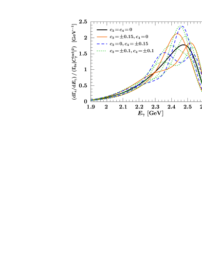
Finally, in Fig. 13 we combine our results to show the $B\to X_{s}\gamma$ spectrum, $(\mathrm{d}\Gamma_{s}/\mathrm{d}E_{\gamma})/\bigl{[}\Gamma_{0s}\,|C_{7}^{\rm incl}(0)|^{2}\bigr{]}$, in the $B$ meson restframe. The results are shown using the short distance parameters $m_{b}^{1S}$ and $\lambda_{1}^{\mathrm{i}}$, and the nine shape function models plotted in Fig. 10, which have fixed zeroth, first, and second moments. The solid black curve is our default model, $\widehat{F}^{\rm mod}(k)$ in Eq. (34). In the current and future experimental analyses $m_{B}-2E_{\gamma}\lesssim 2\,\mathrm{GeV}$. Our formalism has the virtue that we do not need to distinguish regions 1) and 2) in Eq. (II), i.e., it is simultaneously valid for both $m_{B}-2E_{\gamma}^{\mathrm{cut}}\sim\Lambda_{\mathrm{QCD}}$ and $\gg\Lambda_{\mathrm{QCD}}$. The variation of the curves near maximal $E_{\gamma}$ indicates that in the peak region the first few moments of the shape function are not sufficient to predict the spectrum. However, for $E_{\gamma}\lesssim 2.1\,\mathrm{GeV}$, the uncertainty in the prediction becomes significantly smaller, and the leading order shape function model uncertainty diminishes. The spectrum in this region is also affected by subleading shape functions and additional perturbative corrections not studied here. (Note that the measured spectrum is somewhat broadened by experimental effects.) We found the same conclusion using many other shape function models, constructed from different bases, and expect that this will also be substantiated by an actual experimental analysis in which the space of shape functions is explored by allowing for more components in our orthonormal basis and a simultaneous fit to all relevant data. This will have important implications for the $B\to X_{s}\gamma$ rate in the presence of an experimental cut, the extraction of $|V_{ub}|$ from inclusive semileptonic $B$ decays, and the analysis of the inclusive $B\to X_{s}\ell^{+}\ell^{-}$ rate in the small $q^{2}$ region.

VI Conclusions

In this paper, we introduced new methods for calculations relevant for inclusive $B$ decays which involve the parton distribution function of the $b$ quark in a $B$ meson, called the shape function. On the theoretical side, our results allow for an improved description of the decay rates and a more reliable assessment of the uncertainties than earlier studies. On the experimental side, they are straightforward to implement and provide a transparent way to combine constraints on the shape and moments of the shape function, with controllable uncertainties.

The shape function is constrained by the measurements of the shape of the $B\to X_{s}\gamma$ photon energy spectrum Chen:2001fja ; Abe:2008sx ; Aubert:2007my and the $m_{X}$ spectrum in $B\to X_{u}\ell\bar{\nu}$ Aubert:2004bq , and its moments are related to the $b$ quark mass, $m_{b}$, and nonperturbative matrix elements of local operators in the OPE, which are constrained by fits to $B\to X_{c}\ell\bar{\nu}$ decay distributions Bauer:2004ve ; Buchmuller:2005zv ; Barberio:2007cr .

The first key ingredient in our analysis is the new description of the shape function, given in Eq. (2) and discussed in detail in Sec. III, which is by construction consistent with the renormalization group evolution and the perturbative result for the tail of the shape function. It allows combining all experimental information from the shape of $B\to X_{s}\gamma$ and $B\to X_{u}\ell\bar{\nu}$ spectra, and $m_{b}$ and $\lambda_{1}$ constrained by $B\to X_{c}\ell\bar{\nu}$ distributions. Any short distance scheme for the $b$ quark mass and the kinetic energy matrix element can be implemented. We presented a simple formula for the differential rates which incorporates resummed perturbative corrections, with details of the derivation given in Apps. A and B.

The second key ingredient in our analysis is the expansion of the $F$ function, describing the nonperturbative part of the shape function, in a complete set of orthonormal functions in Sec. IV. This gives a new way to quantify uncertainties in the functional form of the shape function, which was previously not explored fully systematically. Choosing $Y(x)$ in Eq. (44) to coincide with any of the models used in the literature DeFazio:1999sv ; Lange:2005yw ; Andersen:2005mj ; Gambino:2007rp ; Aglietti:2007ik gives an orthonormal basis for the shape function in which the first function is the model and corrections can be studied.

One should use renormalon-free short distance definitions for input parameters, such as the $b$ quark mass, $m_{b}$, or the kinetic energy matrix element, $\lambda_{1}$. We found that in our framework the kinetic scheme definition of $\lambda_{1}^{\rm kin}$ seems to oversubtract from the HQET definition of $\lambda_{1}$ in dimensional regularization, numerically similar to using the $\overline{\rm MS}$ mass for inclusive spectra. To solve this problem, in App. C we introduced a new short distance “invisible” scheme, $\lambda_{1}^{\mathrm{i}}$, which is renormalon-free and only differs from the usual definition starting at order $\alpha_{s}^{2}$. While it does not improve the behavior of the perturbation series decisively, being almost invisible, at least it does not make it worse.

It should be emphasized that all developments presented in this paper are consistent with and incorporate all predictions that follow from QCD, without recourse to models or relying on any ad hoc assumptions. In fact, any method consistent with the factorization theorem and the OPE discussed in Sec. II can be cast in our framework.

Our results lead to the following strategy to determine $\lvert V_{ub}\rvert$ with optimal and reliable uncertainties:

1. Fix a basis for the expansion of the $F$ function by choosing a suitable $Y(x)$ and a value for $\lambda$.

2. Do a combined fit to the binned $B\to X_{s}\gamma$ and/or $B\to X_{u}\ell\bar{\nu}$ spectra, and to the information on $m_{b}$ and $\lambda_{1}$ from $B\to X_{c}\ell\bar{\nu}$ (and possibly higher moments) to extract the basis coefficients $\{c_{0},\ldots,c_{N}\}$.

3. Verify that the truncation error is small compared to other uncertainties.

4. Use the values and covariance matrix of the extracted basis coefficients to make predictions with reliable uncertainties.

More details on the shape function fitting procedure, on extracting $|V_{ub}|$ from various $B\to X_{u}\ell\bar{\nu}$ differential decay distributions, and predictions for the $B\to X_{s}\gamma$ rate will be presented elsewhere.

Appendix A Perturbative Results

In this appendix we collect the known results for the hard functions $H_{u,s}(p_{X}^{\pm},\mu_{i})$ in Eq. (4), and derive an analytic result for the function $P(p^{-},p_{X}^{+},\mu_{i})$ in Eq. (II), which includes perturbative corrections from the jet and soft functions as well as the shape function RGE. In Ref. Fleming:2007xt it was shown in the context of dijet production that the convolution form for the soft function analogous to Eq. (21) allows all factors associated with perturbative corrections and RGE to be evaluated analytically. Here we show that this is also true for inclusive $B$ decays. Our calculation differs from Ref. Fleming:2007xt in that we develop a method that avoids using an imaginary part at intermediate steps. (An alternative analytic method that avoids the plus distributions by using moments was developed in Ref. Neubert:2005nt .) Furthermore, with our basis for $\widehat{F}(k)$, we show that the integrals over the basis function can be written in terms of hypergeometric functions.

We discuss fixed order results in Sec. A.1, the RGE in Sec. A.2, and the rate in short distance schemes in Sec. A.3. The definitions of the required plus distributions and many useful relations are collected in App. B.

A.1 Fixed order results

In Eqs. (4) and (II) the leading order hard function $H_{s}(p_{X}^{+},\mu_{i})$ for $B\to X_{s}\gamma$ is

$$H_{s}(p_{X}^{+},\mu_{i}) =\frac{(m_{B}-p_{X}^{+})^{3}}{m_{b}^{3}}\,\lvert C_{7}^{\mathrm{incl}}(0)\rvert^{2}$$

$$\quad\times h_{s}(m_{b},\mu_{b})\,U_{H}(m_{b},\mu_{b},\mu_{i})\,,$$ (65)

where the evolution factor $U_{H}(m_{b},\mu_{b},\mu_{i})$ is given below in Eq. (78), and has the boundary condition $U_{H}(m_{b},\mu_{b},\mu_{b})=1$. The Wilson coefficient $C_{7}^{\mathrm{incl}}$ in $H_{s}$ contains the weak scale matching of the full theory onto the effective Hamiltonian from which the $W$ and $t$ are integrated out, and resums perturbative corrections between the weak scale and the scale $\mu\sim m_{b}$. It does not depend on $\mu_{b}$ and is defined by the split matching procedure in Ref. Lee:2005pk , which separates the perturbation series above and below the scale $m_{b}$. It can be written as Lee:2006gs

$$C_{7}^{\mathrm{incl}}(0)=\mathcal{C}_{7}+F_{7}(0)+G_{7}(0)\,,$$ (66)

with the central values $C_{7}^{\rm incl}(0)=-0.341-0.015i$ and ${\cal C}_{7}=-0.261$. The Wilson coefficient $\mathcal{C}_{7}$ and the functions $F_{7}(q^{2})$ and $G_{7}(q^{2})$ are defined to be separately $\mu$ independent. Here, $\mathcal{C}_{7}$ contains the dependence on the $\overline{\rm MS}$ $b$ quark mass and the Wilson coefficient $C_{7}(\mu)$ from the operator $O_{7}$ in the weak Hamiltonian,

$$\mathcal{C}_{7} =C_{7}(\mu)\,\frac{\overline{m}_{b}(\mu)}{m_{b}}+C_{i}(\mu)\kappa_{i7}$$

$$-\frac{\alpha_{s}(\mu)}{4\pi}\ln\frac{\mu}{m_{b}}\biggl{[}\frac{8}{3}C_{7}(\mu)\frac{\overline{m}_{b}(\mu)}{m_{b}}-\frac{32}{9}C_{8}(\mu)$$

$$+C_{i}(\mu)\Big{(}\gamma_{ij}^{(0)}\kappa_{j7}+\gamma_{i7}^{(0)}\Big{)}\biggr{]}+{\cal O}(\alpha_{s}^{2})\,.$$ (67)

The Wilson coefficients $C_{i}(\mu)$, $\kappa_{i7}$, and the anomalous dimensions $\gamma_{ij}^{(0)}$ are with respect to the operator basis of Ref. Chetyrkin:1996vx and are given explicitly in Ref. Lee:2006gs . The function $F_{7}(q^{2})$ contains perturbative corrections from other operators in the weak Hamiltonian, while $G_{7}(q^{2})$ contains nonperturbative corrections from intermediate $c\bar{c}$ states. They are given in Eqs. (A5) and (A12) in Ref. Lee:2006gs .

The coefficient $h_{s}(m_{b},\mu_{b})$ in Eq. (A.1) corresponds to the matching coefficient for the tensor current in SCET. At $\mathcal{O}(\alpha_{s})$ it was computed in Ref. Bauer:2000yr . To determine the hard matching coefficient at $\mathcal{O}(\alpha_{s}^{2})$ we take the two-loop computation of the $|C_{7}|^{2}$ terms in the $b\to s\gamma$ rate and spectrum from Refs. Blokland:2005uk and subtract the terms in the partonic two-loop spectrum in SCET coming from the jet and shape functions (given by $P(m_{b},k,\mu_{b})$ in Eq. (A.2) below). Due to the split matching, the $\mu_{b}$ dependence in $h_{s}(m_{b},\mu_{b})$ cancels entirely against the $\mu_{b}$ dependence in $U_{H}(m_{b},\mu_{b},\mu_{i})$ in Eq. (A.1), and does not depend on the $\mu$ dependence of the coefficients in the electroweak Hamiltonian. We obtain

$$h_{s}(m_{b},\mu_{b})$$

$$=1-\frac{\alpha_{s}(\mu_{b})}{\pi}\,C_{F}\biggl{(}\ln^{2}\!\frac{\mu_{b}}{m_{b}}+\frac{5}{2}\ln\frac{\mu_{b}}{m_{b}}+3+\frac{\pi^{2}}{24}\biggr{)}$$

$$\quad+\frac{\alpha_{s}^{2}(\mu_{b})}{\pi^{2}}\,C_{F}\biggl{\{}\frac{1}{2}\,C_{F}\ln^{4}\!\frac{\mu_{b}}{m_{b}}+\Bigl{(}\frac{5}{2}\,C_{F}-\frac{1}{6}\,\beta_{0}\Bigr{)}\ln^{3}\!\frac{\mu_{b}}{m_{b}}$$

$$\quad+\biggl{[}\Bigl{(}\frac{49}{8}+\frac{\pi^{2}}{24}\Bigr{)}C_{F}+\Bigl{(}\frac{\pi^{2}}{12}-\frac{1}{3}\Bigr{)}C_{A}-\frac{25}{24}\,\beta_{0}\biggr{]}\ln^{2}\!\frac{\mu_{b}}{m_{b}}$$

$$\quad+\biggl{[}\Bigl{(}\frac{117}{16}+\frac{17\pi^{2}}{48}-3\zeta_{3}\Bigr{)}C_{F}+\Bigl{(}\frac{\pi^{2}}{12}-\frac{29}{72}+\frac{11\zeta_{3}}{4}\Bigr{)}C_{A}$$

$$\quad-\Bigl{(}\frac{341}{144}+\frac{\pi^{2}}{12}\Bigr{)}\beta_{0}\biggr{]}\ln\frac{\mu_{b}}{m_{b}}+3.88611\,C_{F}+5.89413\,C_{A}$$

$$\quad-\Bigl{(}\frac{7859}{3456}+\frac{109\pi^{2}}{576}+\frac{13\zeta_{3}}{48}\Bigr{)}\beta_{0}+\frac{3563}{1296}-\frac{29\pi^{2}}{108}-\frac{\zeta_{3}}{6}\biggr{\}}\,.$$ (68)

Our expressions here agree with the corresponding numerical results in Eq. $(99)$ of Ref. Ali:2007sj . Note that the inverse powers of $m_{b}$ in Eqs. (A.1), (A.1), and (A.1) below cancel the $m_{b}^{5}$ factors in $\Gamma_{0s,u}$ in Eq. (5), and any mass scheme can be used. The $m_{b}$ appearing in $h_{s}(m_{b},\mu_{b})$ and $U_{H}(m_{b},\mu_{b},\mu_{i})$ is defined in the pole scheme. Here, the pole mass renormalon ambiguity is less relevant, because $m_{b}$ only appears as a reference scale for $\mu_{b}$, so the effect of changing $m_{b}$ is included in the variation of $\mu_{b}$. For numerical calculations, we use $m_{b}=4.7\,\mathrm{GeV}$.

The hard function $H_{u}(E_{\ell},p_{X}^{-},p_{X}^{+},\mu_{i})$ for $B\to X_{u}\ell\bar{\nu}$ in Eqs. (4) and (II) is given by

$$H_{u}(E_{\ell},p_{X}^{-},p_{X}^{+},\mu_{i})=\frac{24}{m_{b}^{5}}\big{(}m_{B}-p_{X}^{+}\big{)}\big{(}2E_{\ell}+p_{X}^{-}-m_{B}\big{)}$$

$$\times\biggl{\{}\big{(}2m_{B}-p_{X}^{+}-p_{X}^{-}-2E_{\ell}\big{)}\,h_{u1}(m_{b},p^{-},\mu_{b})$$

$$\quad+\big{(}m_{B}-p_{X}^{+}-2E_{\ell}\big{)}\biggl{[}h_{u2}(m_{b},p^{-},\mu_{b})$$

$$\quad+\frac{m_{B}-p_{X}^{+}}{p_{X}^{-}-p_{X}^{+}}\,h_{u3}(m_{b},p^{-},\mu_{b})\biggr{]}\biggr{\}}\,U_{H}(p^{-},\mu_{b},\mu_{i})\,,$$ (69)

where the $h_{ui}(m_{b},p^{-},\mu_{b})$ correspond to the matching coefficients of the $V-A$ current in SCET. To order $\alpha_{s}$ Bauer:2000yr ; Bauer:2003pi ; Bosch:2004th

$$h_{u1}(m_{b},p^{-},\mu_{b})$$

$$\quad=1-\frac{\alpha_{s}(\mu_{b})}{\pi}\,C_{F}\biggl{[}\ln^{2}\!\frac{\mu_{b}}{p^{-}}+\frac{5}{2}\ln\frac{\mu_{b}}{m_{b}}+{\rm Li}_{2}\Big{(}1-\frac{p^{-}}{m_{b}}\Big{)}$$

$$\qquad+\frac{3p^{-}-2m_{b}}{2m_{b}-2p^{-}}\,\ln\frac{p^{-}}{m_{b}}+\frac{\pi^{2}}{24}+3\biggr{]}\,,$$

$$h_{u2}(m_{b},p^{-},\mu_{b})$$

$$\quad=\frac{\alpha_{s}(\mu_{b})}{2\pi}\,C_{F}\,\frac{m_{b}}{m_{b}-p^{-}}\biggl{(}\frac{p^{-}}{m_{b}-p^{-}}\ln\frac{p^{-}}{m_{b}}+1\biggr{)}\,,$$

$$h_{u3}(m_{b},p^{-},\mu_{b})$$ (70)

$$\quad=\frac{\alpha_{s}(\mu_{b})}{2\pi}\,C_{F}\frac{p^{-}}{m_{b}-p^{-}}\biggl{(}\frac{m_{b}-2p^{-}}{m_{b}-p^{-}}\ln\frac{p^{-}}{m_{b}}-1\biggr{)}\,.$$

The corresponding two-loop results for $H_{u}$ will be easy to implement once they become available. Finally, the evolution factor $U_{H}(p^{-},\mu_{b},\mu_{i})$ in Eq. (A.1) is identical for $H_{s}$ and $H_{u}$, and is given below in Eq. (78).

We now turn to the function $P(p^{-},k,\mu_{i})$ in Eq. (II). Changing variables $\omega\to\omega^{\prime}+k-\omega$, we have

$$P(p^{-},k,\mu_{i}) =\!\int\!\mathrm{d}\omega\,U_{S}(k-\omega,\mu_{i},\mu_{\Lambda})$$ (71)

$$\quad\times\!\int\!\mathrm{d}\omega^{\prime}\,p^{-}J[p^{-}(\omega-\omega^{\prime}),\mu_{i}]\,C_{0}(\omega^{\prime},\mu_{\Lambda})\,.$$

To incorporate the fixed order $\alpha_{s}$ corrections to the jet function, $J(p^{2},\mu_{i})$, and the shape function kernel, $C_{0}(\omega,\mu_{\Lambda})$, we will first carry out the $\omega^{\prime}$ convolution integral. The evolution factor $U_{S}(p_{X}^{+},\mu_{i},\mu_{\Lambda})$, which sums logarithms between the scales $\mu_{i}$ and $\mu_{\Lambda}$, and the integral over $\omega$ are discussed later.

To all orders in perturbation theory the jet function and shape function kernel can be written as

$$J(p^{2},\mu_{i}) =\frac{1}{\mu_{i}^{2}}\sum_{n=-1}^{\infty}J_{n}[\alpha_{s}(\mu_{i})]\,\mathcal{L}_{n}(p^{2}/\mu_{i}^{2})\,,$$

$$C_{0}(\omega,\mu_{\Lambda}) =\frac{1}{\mu_{\Lambda}}\sum_{n=-1}^{\infty}S_{n}[\alpha_{s}(\mu_{\Lambda})]\,\mathcal{L}_{n}(\omega/\mu_{\Lambda})\,,$$ (72)

where the $\mathcal{L}_{n}(x)$ are plus distributions defined in Eq. (108) for $n\geq 0$ and in Eq. (112) for $n=-1$, and the coefficients $J_{n}(\alpha_{s})$ and $S_{n}(\alpha_{s})$ have expansions in $\alpha_{s}$. The jet function coefficients are known at one Bauer:2003pi and two loops Becher:2006qw , and are given by

$$J_{-1}(\alpha_{s}) =1+\frac{\alpha_{s}}{\pi}\,\Bigl{(}\frac{7}{4}-\frac{\pi^{2}}{4}\Bigr{)}C_{F}$$

$$\quad+\frac{\alpha_{s}^{2}}{\pi^{2}}\biggl{[}\Bigl{(}\frac{205}{128}-\frac{67\pi^{2}}{96}+\frac{7\pi^{4}}{120}-\frac{9\zeta_{3}}{8}\Bigr{)}C_{F}^{2}$$

$$\quad\quad+\Bigl{(}\frac{1417}{1728}-\frac{7\pi^{2}}{144}-\frac{17\pi^{4}}{2880}-\frac{9\zeta_{3}}{8}\Bigr{)}C_{F}C_{A}$$

$$\qquad+\Bigl{(}\frac{4057}{3456}-\frac{17\pi^{4}}{144}-\frac{\zeta_{3}}{12}\Bigr{)}C_{F}\beta_{0}\biggr{]}\,,$$

$$J_{0}(\alpha_{s}) =-\frac{\alpha_{s}}{\pi}\,\frac{3}{4}\,C_{F}-\frac{\alpha_{s}^{2}}{\pi^{2}}\biggl{[}\Bigl{(}\frac{45}{32}-\frac{7\pi^{2}}{16}+\frac{\zeta_{3}}{2}\Bigr{)}C_{F}^{2}$$

$$\quad+\Bigl{(}\frac{73}{144}-\frac{5\zeta_{3}}{2}\Bigr{)}C_{F}C_{A}+\Bigl{(}\frac{247}{288}-\frac{\pi^{2}}{24}\Bigr{)}C_{F}\beta_{0}\biggr{]}\,,$$

$$J_{1}(\alpha_{s}) =\frac{\alpha_{s}}{\pi}\,C_{F}+\frac{\alpha_{s}^{2}}{\pi^{2}}\biggr{[}\Bigl{(}\frac{37}{16}-\frac{5\pi^{2}}{12}\Bigr{)}C_{F}^{2}$$

$$\quad+\Bigl{(}\frac{1}{3}-\frac{\pi^{2}}{12}\Bigr{)}C_{F}C_{A}+\frac{29}{48}\,C_{F}\beta_{0}\biggl{]}\,,$$

$$J_{2}(\alpha_{s}) =-\frac{\alpha_{s}^{2}}{\pi^{2}}\,\Bigl{(}\frac{9}{8}\,C_{F}^{2}+\frac{1}{8}\,C_{F}\beta_{0}\Bigr{)}\,,$$

$$J_{3}(\alpha_{s}) =\frac{\alpha_{s}^{2}}{\pi^{2}}\,\frac{1}{2}\,C_{F}^{2}\,.$$ (73)

The shape function coefficients to one Bauer:2003pi and two loops Becher:2005pd are

$$S_{-1}(\alpha_{s}) =1-\frac{\alpha_{s}}{\pi}\,\frac{\pi^{2}}{24}\,C_{F}-\frac{\alpha_{s}^{2}}{\pi^{2}}\biggr{[}\Bigl{(}\frac{\pi^{2}}{12}+\frac{3\pi^{4}}{640}-2\zeta_{3}\Bigr{)}C_{F}^{2}$$

$$\quad+\Bigl{(}\frac{29}{108}+\frac{31\pi^{2}}{144}-\frac{67\pi^{4}}{2880}+\frac{9\zeta_{3}}{8}\Bigr{)}C_{F}C_{A}$$

$$\quad+\Bigl{(}-\frac{1}{216}+\frac{5\pi^{2}}{576}-\frac{5\zeta_{3}}{48}\Bigr{)}C_{F}\beta_{0}\biggl{]}\,,$$

$$S_{0}(\alpha_{s}) =-\frac{\alpha_{s}}{\pi}\,C_{F}+\frac{\alpha_{s}^{2}}{\pi^{2}}\biggr{[}\Bigl{(}-\frac{7\pi^{2}}{24}+4\zeta_{3}\Bigr{)}C_{F}^{2}$$

$$\quad+\Bigl{(}\frac{11}{18}+\frac{\pi^{2}}{12}-\frac{9\zeta_{3}}{4}\Bigr{)}C_{F}C_{A}-\frac{1}{36}\,C_{F}\beta_{0}\biggl{]}\,,$$

$$S_{1}(\alpha_{s}) =-\frac{\alpha_{s}}{\pi}\,2C_{F}+\frac{\alpha_{s}^{2}}{\pi^{2}}\biggr{[}\Bigl{(}1-\frac{7\pi^{2}}{12}\Bigr{)}C_{F}^{2}$$

$$\quad+\Bigl{(}-\frac{2}{3}+\frac{\pi^{2}}{6}\Bigr{)}C_{F}C_{A}-\frac{1}{3}\,C_{F}\beta_{0}\biggl{]}\,,$$

$$S_{2}(\alpha_{s}) =\frac{\alpha_{s}^{2}}{\pi^{2}}\,\Bigl{(}3C_{F}^{2}+\frac{1}{2}\,C_{F}\beta_{0}\Bigr{)}\,,$$

$$S_{3}(\alpha_{s}) =\frac{\alpha_{s}^{2}}{\pi^{2}}\,2C_{F}^{2}\,.$$ (74)

All other coefficients in $J$ and $C_{0}$ start at higher orders in $\alpha_{s}$.

To convolute $\mathcal{L}_{n}[p^{-}(\omega-\omega^{\prime})/\mu_{i}^{2}]$ with $\mathcal{L}_{m}(\omega/\mu_{\Lambda})$ we first rescale them to have the same dimensionless arguments. Using Eq. (115), $J$ and $C_{0}$ satisfy the rescaling identities

$$J(p^{-}\omega,\mu) =\frac{1}{p^{-}\xi}\sum_{n=-1}^{\infty}J_{n}\Bigl{[}\alpha_{s}(\mu),\frac{p^{-}\xi}{\mu^{2}}\Bigr{]}\,\mathcal{L}_{n}\Bigl{(}\frac{\omega}{\xi}\Bigr{)}\,,$$

$$C_{0}(\omega,\mu) =\frac{1}{\xi}\sum_{n=-1}^{\infty}S_{n}\Bigl{[}\alpha_{s}(\mu),\frac{\xi}{\mu}\Bigr{]}\,\mathcal{L}_{n}\Bigl{(}\frac{\omega}{\xi}\Bigr{)}\,.$$ (75)

where $\xi$ is an arbitrary dimension-one parameter that we will choose at our convenience later on, and the rescaled coefficients are

$$J_{-1}(\alpha_{s},x) =J_{-1}(\alpha_{s})+\sum_{n=0}^{\infty}J_{n}(\alpha_{s})\,\frac{\ln^{n+1}x}{n+1}\,,$$

$$J_{n}(\alpha_{s},x) =\sum_{k=0}^{\infty}\frac{(n+k)!}{n!\,k!}\,J_{n+k}(\alpha_{s})\,\ln^{k}x\,,$$

$$S_{-1}(\alpha_{s},x) =S_{-1}(\alpha_{s})+\sum_{n=0}^{\infty}S_{n}(\alpha_{s})\,\frac{\ln^{n+1}x}{n+1}\,,$$

$$S_{n}(\alpha_{s},x) =\sum_{k=0}^{\infty}\frac{(n+k)!}{n!\,k!}\,S_{n+k}(\alpha_{s})\,\ln^{k}x\,.$$ (76)

Using Eq. (A.1), the convolution of $J$ and $C_{0}$ in Eq. (71) becomes

$$(J\otimes C_{0})(\omega,\mu_{i},\mu_{\Lambda})$$

$$\equiv\!\int\!\mathrm{d}\omega^{\prime}\,p^{-}J[p^{-}(\omega-\omega^{\prime}),\mu_{i}]\,C_{0}(\omega^{\prime},\mu_{\Lambda})$$

$$=\sum_{m,n=-1}^{\infty}\!J_{m}\Bigl{[}\alpha_{s}(\mu_{i}),\frac{p^{-}\xi}{\mu_{i}^{2}}\Bigr{]}\,S_{n}\Bigl{[}\alpha_{s}(\mu_{\Lambda}),\frac{\xi}{\mu_{\Lambda}}\Bigr{]}$$

$$\quad\times\frac{1}{\xi}\int\!\mathrm{d}x\,\mathcal{L}_{m}\Bigl{(}\frac{\omega}{\xi}-x\Bigr{)}\,\mathcal{L}_{n}(x)$$

$$=\sum_{\ell=-1}^{\infty}\!\sum_{\begin{subarray}{c}m,n\geq-1\\ m+n+1\geq\ell\end{subarray}}^{\infty}\!V^{mn}_{\ell}J_{m}\Bigl{[}\alpha_{s}(\mu_{i}),\frac{p^{-}\xi}{\mu_{i}^{2}}\Bigr{]}\,S_{n}\Bigl{[}\alpha_{s}(\mu_{\Lambda}),\frac{\xi}{\mu_{\Lambda}}\Bigr{]}$$

$$\quad\times\frac{1}{\xi}\,\mathcal{L}_{\ell}\Bigr{(}\frac{\omega}{\xi}\Bigr{)}\,.$$ (77)

In the last step we used Eq. (B) to perform the $x$ integral, yielding a sum of plus distributions, whose coefficients $V_{\ell}^{mn}$ are given in Eq. (119).

A.2 Renormalization group evolution

Next, we summarize results for the renormalization group evolution, and then carry out the $\omega$ integral in Eq. (71). The factor $U_{H}(p^{-},\mu_{b},\mu_{i})$ which describes the evolution of the hard functions in Eqs. (A.1) and (A.1) between the hard scale, $\mu_{b}$, and the jet scale, $\mu_{i}$, is Bauer:2000yr

$$U_{H}(p^{-},\mu_{b},\mu_{i})=e^{K_{H}(\mu_{i},\mu_{b})}\,\bigg{(}\frac{p^{-}}{\mu_{b}}\bigg{)}^{\eta(\mu_{i},\mu_{b})}\,,$$ (78)

where definitions of $\eta(\mu_{i},\mu_{b})$ and $K_{H}(\mu_{i},\mu_{b})$ are given in Eq. (A.2) below. The soft evolution factor $U_{S}(\omega,\mu_{i},\mu_{\Lambda})$ in Eq. (71) sums logarithms between the jet scale, $\mu_{i}$, and soft scale, $\mu_{\Lambda}$. To all orders in perturbation theory it can be written as

$$U_{S}(\omega,\mu_{i},\mu_{\Lambda})=e^{K_{S}(\mu_{i},\mu_{\Lambda})}\frac{e^{-\gamma_{E}\eta}}{\Gamma(\eta)}\frac{1}{\mu_{\Lambda}}\biggr{[}\frac{\theta(\omega/\mu_{\Lambda})}{(\omega/\mu_{\Lambda})^{1-\eta}}\biggl{]}_{+}^{\text{\footnotesize Ref.\,\cite[cite]{\@@bibref{Authors Phrase1YearPhrase2}{Fleming:2007xt}{\@@citephrase{(}}{\@@citephrase{)}}}}}$$

$$\quad=E_{S}(\xi,\mu_{i},\mu_{\Lambda})\,\frac{1}{\xi}\Bigl{[}\eta\,\mathcal{L}^{\eta}\Big{(}\frac{\omega}{\xi}\Big{)}+\,\mathcal{L}_{-1}\Big{(}\frac{\omega}{\xi}\Big{)}\Bigr{]}\,,$$ (79)

where $\eta\equiv\eta(\mu_{i},\mu_{\Lambda})$, and we defined

$$E_{S}(\xi,\mu_{i},\mu_{\Lambda})=e^{K_{S}(\mu_{i},\mu_{\Lambda})}\,\Bigl{(}\frac{\xi}{\mu_{\Lambda}}\Bigr{)}^{\eta}\ \frac{e^{-\gamma_{E}\,\eta}}{\Gamma(1+\eta)}\,.$$ (80)

To go from the first to the second line in Eq. (A.2) we used Eqs. (110) and (114). An expression for $U_{S}(\omega,\mu_{i},\mu_{\Lambda})$ was first found in Ref. Balzereit:1998yf and extended to all orders in Ref. Neubert:2004dd . The form with the plus distribution derived in Ref. Fleming:2007xt makes the formula valid without having to require $\mu_{i}>\mu_{\Lambda}$.

In Eqs. (78) to (80), $\eta(\mu,\mu_{0})$ and $K_{x}(\mu,\mu_{0})$ for $x=H$ or $S$ are given to all orders by

$$\eta(\mu,\mu_{0}) =2\int_{\alpha_{s}(\mu_{0})}^{\alpha_{s}(\mu)}\!\mathrm{d}\alpha_{s}\,\frac{\Gamma_{\mathrm{cusp}}(\alpha_{s})}{\beta(\alpha_{s})}\,,$$

$$K_{x}(\mu,\mu_{0}) =-2\int_{\alpha_{s}(\mu_{0})}^{\alpha_{s}(\mu)}\!\mathrm{d}\alpha_{s}\,\biggl{[}\frac{\Gamma_{\mathrm{cusp}}(\alpha_{s})}{\beta(\alpha_{s})}$$

$$\qquad\times\int_{\alpha_{s}(\mu_{0})}^{\alpha_{s}}\frac{\mathrm{d}\alpha_{s}^{\prime}}{\beta(\alpha_{s}^{\prime})}+\frac{\gamma_{x}(\alpha_{s})}{\beta(\alpha_{s})}\biggl{]}\,.$$ (81)

Here, $\Gamma_{\mathrm{cusp}}$ is the universal cusp anomalous dimension. The only difference between $K_{H}$ and $K_{S}$ are the hard and soft anomalous dimensions, $\gamma_{x}=\gamma_{S}$ or $\gamma_{H}$. Expanding the $\beta$ function and anomalous dimensions as usual,

$$\beta(\alpha_{s}) =-2\alpha_{s}\sum_{n=0}^{\infty}\beta_{n}\Bigl{(}\frac{\alpha_{s}}{4\pi}\Bigr{)}^{n+1}\,,$$

$$\Gamma_{\rm cusp}(\alpha_{s}) =\sum_{n=0}^{\infty}\Gamma_{n}\Bigl{(}\frac{\alpha_{s}}{4\pi}\Bigr{)}^{n+1}\,,$$

$$\gamma_{x}(\alpha_{s}) =\sum_{n=0}^{\infty}\gamma^{x}_{n}\Bigl{(}\frac{\alpha_{s}}{4\pi}\Bigr{)}^{n+1}\,,$$ (82)

the integrals in Eq. (A.2) to NNLL are

$$\eta(\mu,\mu_{0}) =-\frac{\Gamma_{0}}{\beta_{0}}\,\biggl{[}\ln r+\frac{\alpha_{s}(\mu_{0})}{4\pi}\,\biggl{(}\frac{\Gamma_{1}}{\Gamma_{0}}-\frac{\beta_{1}}{\beta_{0}}\biggr{)}(r-1)+\frac{\alpha_{s}^{2}(\mu_{0})}{16\pi^{2}}\biggl{(}\frac{\Gamma_{2}}{\Gamma_{0}}-\frac{\beta_{1}\Gamma_{1}}{\beta_{0}\Gamma_{0}}+\frac{\beta_{1}^{2}}{\beta_{0}^{2}}-\frac{\beta_{2}}{\beta_{0}}\biggr{)}\frac{r^{2}-1}{2}\biggr{]}\,,$$

$$K_{x}(\mu,\mu_{0}) =\frac{\Gamma_{0}}{2\beta_{0}^{2}}\,\biggl{\{}\frac{4\pi}{\alpha_{s}(\mu_{0})}\,\Bigl{(}1-\frac{1}{r}-\ln r\Bigr{)}+\biggl{(}\frac{\Gamma_{1}}{\Gamma_{0}}-\frac{\beta_{1}}{\beta_{0}}\biggr{)}(1-r+\ln r)+\frac{\beta_{1}}{2\beta_{0}}\ln^{2}r+\frac{2\beta_{0}\gamma_{0}^{x}}{\Gamma_{0}}\,\ln r$$

$$\quad+\frac{\alpha_{s}(\mu_{0})}{4\pi}\,\biggl{[}\biggl{(}\frac{\beta_{1}^{2}}{\beta_{0}^{2}}-\frac{\beta_{2}}{\beta_{0}}\biggr{)}\Bigl{(}\frac{1-r^{2}}{2}+\ln r\Bigr{)}+\biggl{(}\frac{\beta_{1}\Gamma_{1}}{\beta_{0}\Gamma_{0}}-\frac{\beta_{1}^{2}}{\beta_{0}^{2}}\biggr{)}(1-r+r\ln r)-\biggl{(}\frac{\Gamma_{2}}{\Gamma_{0}}-\frac{\beta_{1}\Gamma_{1}}{\beta_{0}\Gamma_{0}}\biggr{)}\frac{(1-r)^{2}}{2}$$

$$\qquad+\frac{2\beta_{0}\gamma_{0}^{x}}{\Gamma_{0}}\,\biggl{(}\frac{\gamma_{1}^{x}}{\gamma_{0}^{x}}-\frac{\beta_{1}}{\beta_{0}}\biggr{)}(r-1)\biggr{]}\biggr{\}}\,,$$ (83)

with $r=\alpha_{s}(\mu)/\alpha_{s}(\mu_{0})$. When using $\eta(\mu,\mu_{0})$ and $K_{x}(\mu,\mu_{0})$ at LL, NLL, and NNLL according to our conventions in Eq. (25), we do not re-expand the results in Eqs. (78) and (80), but keep their full expressions everywhere. For the running coupling we always use the three-loop expression

$$\frac{1}{\alpha_{s}(\mu)}=\frac{X}{\alpha_{s}(\mu_{0})}+\frac{\beta_{1}}{4\pi\beta_{0}}\ln X+\frac{\alpha_{s}(\mu_{0})}{16\pi^{2}}\biggr{[}\frac{\beta_{2}}{\beta_{0}}\Bigl{(}1-\frac{1}{X}\Bigr{)}+\frac{\beta_{1}^{2}}{\beta_{0}^{2}}\Bigl{(}\frac{\ln X}{X}+\frac{1}{X}-1\Bigr{)}\biggl{]}\,,$$ (84)

where $X\equiv 1+\alpha_{s}(\mu_{0})\beta_{0}\ln(\mu/\mu_{0})/(2\pi)$, and we evolve to lower scales using the reference value $\alpha_{s}(\mu_{0}=4.7\,{\rm GeV})=0.2155$ as in Table 1 with $n_{f}=4$. Up to three-loop order, the coefficients of the $\beta$ function in the $\overline{\rm MS}$ scheme are

$$\beta_{0} =\frac{11}{3}\,C_{A}-\frac{2}{3}\,n_{f}\,,$$

$$\beta_{1} =\frac{34}{3}\,C_{A}^{2}-\frac{10}{3}\,C_{A}\,n_{f}-2C_{F}\,n_{f}\,,$$

$$\beta_{2} =\frac{2857}{54}\,C_{A}^{3}+\Bigl{(}C_{F}^{2}-\frac{205}{18}\,C_{F}C_{A}-\frac{1415}{54}\,C_{A}^{2}\Bigr{)}\,n_{f}$$

$$\quad+\Bigl{(}\frac{11}{9}\,C_{F}+\frac{79}{54}\,C_{A}\Bigr{)}\,n_{f}^{2}\,.$$ (85)

The cusp Korchemsky:1987wg ; Moch:2004pa , soft Korchemsky:1992xv ; Gardi:2005yi , and hard anomalous dimension coefficients are

$$\Gamma_{0} =4C_{F}\,,$$

$$\Gamma_{1} =\Bigl{(}\frac{268}{9}-\frac{4\pi^{2}}{3}\Bigr{)}\,C_{F}C_{A}-\frac{40}{9}C_{F}\,n_{f}\,,$$

$$\Gamma_{2} =\Bigl{(}\frac{490}{3}-\frac{536\pi^{2}}{27}+\frac{44\pi^{4}}{45}+\frac{88\zeta_{3}}{3}\Bigr{)}C_{F}C_{A}^{2}$$

$$\quad+\Bigl{(}\frac{80\pi^{2}}{27}-\frac{836}{27}-\frac{112\zeta_{3}}{3}\Bigr{)}C_{F}C_{A}\,n_{f}$$

$$\quad+\Bigl{(}32\zeta_{3}-\frac{110}{3}\Bigr{)}C_{F}^{2}\,n_{f}-\frac{16}{27}\,C_{F}\,n_{f}^{2}\,,$$

$$\gamma_{0}^{S} =-2C_{F}\,,$$

$$\gamma_{1}^{S} =\Bigl{(}\frac{110}{27}+\frac{\pi^{2}}{18}-18\zeta_{3}\Bigr{)}C_{F}C_{A}+\Bigl{(}\frac{4}{27}+\frac{\pi^{2}}{9}\Bigr{)}C_{F}\,n_{f}\,,$$

$$\gamma_{0}^{H} =5C_{F}\,,$$

$$\gamma_{1}^{H} =\Bigl{(}\frac{3}{2}-2\pi^{2}+24\zeta_{3}\Bigr{)}C_{F}^{2}-\Bigl{(}\frac{125}{27}+\frac{\pi^{2}}{3}\Bigr{)}C_{F}\,n_{f}$$

$$\quad+\Bigl{(}\frac{1549}{54}+\frac{7\pi^{2}}{6}-22\zeta_{3}\Bigr{)}C_{F}C_{A}\,.$$ (86)

To determine $\gamma_{1}^{H}$ we used $\gamma_{1}^{H}=-\gamma_{1}^{J}-\gamma_{1}^{S}$, which follows from the $\mu$ independence of $\mathrm{d}\Gamma_{s}/\mathrm{d}E_{\gamma}$. We use the two-loop computation of $\gamma_{1}^{J}$ in Ref. Becher:2006qw .

The evolution of the shape function kernel $C_{0}(\omega,\mu)$ from $\mu_{\Lambda}$ to $\mu_{i}$ can be written as the sum of a finite number of terms,

$$C_{0}(\omega,\mu_{i}) =\int\!\mathrm{d}\omega^{\prime}\,U_{S}(\omega-\omega^{\prime},\mu_{i},\mu_{\Lambda})\,C_{0}(\omega^{\prime},\mu_{\Lambda})$$

$$=E_{S}(\xi,\mu_{i},\mu_{\Lambda})\sum_{n=-1}^{\infty}S_{n}\Bigl{[}\alpha_{s}(\mu_{\Lambda}),\frac{\xi}{\mu_{\Lambda}}\Bigr{]}$$

$$\quad\times\frac{1}{\xi}\,\biggl{[}\eta\int\!\mathrm{d}x\,\mathcal{L}^{\eta}\Bigl{(}\frac{\omega}{\xi}-x\Bigr{)}\,\mathcal{L}_{n}(x)+\,\mathcal{L}_{n}\Bigl{(}\frac{\omega}{\xi}\Bigr{)}\biggr{]}$$

$$=E_{S}(\xi,\mu_{i},\mu_{\Lambda})\sum_{n=-1}^{\infty}\,\sum_{\ell=-1}^{n+1}V^{n}_{\ell}(\eta)$$

$$\quad\times S_{n}\Bigl{[}\alpha_{s}(\mu_{\Lambda}),\frac{\xi}{\mu_{\Lambda}}\Bigr{]}\,\frac{1}{\xi}\,\mathcal{L}_{\ell}^{\eta}\Bigl{(}\frac{\omega}{\xi}\Bigr{)}\,.$$ (87)

In the last step, we used Eq. (B) to perform the $x$ integral. The coefficients of the resulting plus distributions, $V_{\ell}^{n}(\eta)$, are defined in Eq. (119). If $C_{0}(\omega,\mu)$ is known to $\mathcal{O}(\alpha_{s}^{k})$ accuracy, then the terms contributing in Eq. (A.2) are bounded by $n\leq 2k-1$. To obtain the shape function evolved up to $\mu_{i}$, $S(\omega,\mu_{i})$, we combine Eq. (21) with (A.2) taking for convenience $\xi=\omega$ and changing the integration variable to $z$ via $k=\omega(1-z)$. This gives the result for $S(\omega,\mu_{i})$ that is quoted in Eq. (24) in the text.

Returning to $P(p^{-},k,\mu_{i})$ in Eq. (71), to perform the $\omega$ integral we can now apply the same steps as in Eq. (A.2) to compute the convolution of $U_{S}(\omega,\mu_{i},\mu_{\Lambda})$ with the result of Eq. (A.1). This yields

$$P(p^{-},k,\mu_{i}) =\sum_{j=-1}^{\infty}P_{j}(p^{-},\xi,\mu_{i},\mu_{\Lambda})\,\frac{1}{\xi}\,\mathcal{L}_{j}^{\eta}\Bigl{(}\frac{k}{\xi}\Bigr{)}\,,$$ (88)

where $\eta=\eta(\mu_{i},\mu_{\Lambda})$, and the coefficients are

$$P_{j}(p^{-},\xi,\mu_{i},\mu_{\Lambda})$$

$$\quad=E_{S}(\xi,\mu_{i},\mu_{\Lambda})\sum_{\begin{subarray}{c}m,n\geq-1\\ m+n+2\geq j\end{subarray}}^{\infty}\biggl{\{}\sum_{\begin{subarray}{c}\ell\geq-1\\ \ell\geq j-1\end{subarray}}^{m+n+1}V^{mn}_{\ell}\,V^{\ell}_{j}(\eta)$$

$$\qquad\times J_{m}\Bigl{[}\alpha_{s}(\mu_{i}),\frac{p^{-}\xi}{\mu_{i}^{2}}\Bigr{]}S_{n}\Bigl{[}\alpha_{s}(\mu_{\Lambda}),\frac{\xi}{\mu_{\Lambda}}\Bigr{]}\biggr{\}}\,,$$ (89)

with $V_{j}^{\ell}(\eta)$ and $V_{\ell}^{mn}$ given in Eqs. (119) and (120). The jet and shape function coefficients, $J_{m}$ and $S_{n}$, have perturbative expansions in $\alpha_{s}(\mu_{i})$ and $\alpha_{s}(\mu_{\Lambda})$, respectively, given by Eqs. (A.1) and (A.1) together with Eq. (A.1). To $\mathcal{O}(\alpha_{s})$ we have $m,n\leq 1$, so dropping cross terms of $\mathcal{O}(\alpha_{s}^{2})$ and higher, we need $-1\leq\ell\leq 1$ and $-1\leq j\leq 2$. To $\mathcal{O}(\alpha_{s}^{2})$, we have $m,n\leq 3$, and we need cross terms between $J_{m}$ and $S_{n}$ up to $-1\leq\ell\leq 3$ and $-1\leq j\leq 4$.

The final step now is to compute the convolution of $P(p^{-},k,\mu_{i})$ with some function $F(k)$,

$$\int\!\mathrm{d}k\,P(p^{-},k,\mu_{i})\,F(p_{X}^{+}-k)$$ (90)

$$\quad=\sum_{j=-1}^{\infty}P_{j}(p^{-},p_{X}^{+},\mu_{i},\mu_{\Lambda})\int_{0}^{1}\!\mathrm{d}z\,\mathcal{L}_{j}^{\eta}(z)\,F[p_{X}^{+}(1-z)]\,.$$

In both Eqs. (24) and (90) the remaining integral that needs to be performed is $\mathcal{L}_{j}^{\eta}(z)$ with $F[\omega(1-z)]$. For $j\geq 0$ it is convenient to simplify this integral to

$$\int_{0}^{1}\!\mathrm{d}z\,\mathcal{L}_{j}^{\eta}(z)\,F[\omega(1-z)]$$ (91)

$$\quad=\int_{0}^{1}\!\mathrm{d}z\,\frac{\ln^{j}z}{z^{1-\eta}}\,\bigl{\{}F[\omega(1-z)]-F(\omega)\bigr{\}}$$

$$\quad=\frac{1}{\eta^{1+j}}\int_{0}^{1}\!\mathrm{d}t\,\ln^{j}t\,\bigl{\{}F\big{[}\omega\big{(}1-t^{1/\eta}\big{)}\big{]}-F(\omega)\bigr{\}}\,,$$

where the second line is valid for $\eta>-1$, but the last line only for $\eta>0$. For $j=-1$ the integral is trivial since ${\cal L}_{-1}^{\eta}(z)=\delta(z)$. Our basis for $F(k)$ involves a series of terms of the form

$$F(k)=\sum_{r,s}C_{rs}\Bigl{(}\frac{k}{\lambda}\Bigr{)}^{r}\exp\Bigl{(}-s\,\frac{k}{\lambda}\Bigr{)}\,,$$ (92)

where $r$ and $s$ are integers. For each term in the series the integral in Eq. (91) can be performed analytically using

$$\int_{0}^{1}\!\mathrm{d}z\,\bigl{[}(1-z)^{\ell}e^{b\,z}-1\bigr{]}\,z^{a+\eta-1}=-\frac{1}{a+\eta}$$ (93)

$$\qquad+\frac{\Gamma(a+\eta)\,\Gamma(1+\ell)}{\Gamma(1+a+\eta+\ell)}\,{}_{1}{}F_{1}(a+\eta,1+a+\eta+\ell,b)\,.$$

By taking derivatives of this result with respect to $a$ one can obtain the integral with $(\ln z)^{j}$ on the left-hand side. In practice, we find that the numerical integration of Eq. (91) is sufficiently fast that using Eq. (93) is unnecessary.

Finally, we comment on a special case of the above results that was used to carry out the $B\to X_{s}\gamma$ matching computation to derive Eq. (A.1). Here we used the SCET computation of the decay rate with $\mu_{b}=\mu_{i}=\mu_{\Lambda}=m_{b}$ and $\eta=0$, which depends on $P(m_{b},p_{X}^{+},m_{b})$. For this special case, the choice $\xi=m_{b}$ is convenient and Eqs. (88) and (A.2) then reduce to

$$P(m_{b},p_{X}^{+},m_{b})=\sum_{j=-1}^{\infty}P_{j}(m_{b},m_{b},m_{b},m_{b})\frac{1}{m_{b}}{\cal L}_{j}\Big{(}\frac{p_{X}^{+}}{m_{b}}\Big{)}\,,$$

$$P_{j}(m_{b},m_{b},m_{b},m_{b})=\!\!\!\!\!\!\sum_{\begin{subarray}{c}m,n\geq-1\\ m+n+2\geq j\end{subarray}}^{\infty}\!\!\!\!\!V^{mn}_{j}J_{m}\big{[}\alpha_{s}(m_{b})\big{]}S_{n}\big{[}\alpha_{s}(m_{b})\big{]}.$$ (94)

Thus $P_{j}(m_{b},m_{b},m_{b},m_{b})$ is the coefficient of the plus distribution or $\delta$ distribution $\mathcal{L}_{j}$ in the fixed-order computation evaluated at $\mu=m_{b}$.

A.3 Changing to short distance schemes

To change the scheme from the pole scheme to a short distance scheme, we define a perturbative function $\widehat{P}$ as in Eq. (II), but with $C_{0}$ replaced by $\widehat{C}_{0}$, and in the differential spectrum $P$ and $F$ are replaced by $\widehat{P}$ and $\widehat{F}$. Displaying only the integration variables,

$$\mathrm{d}\Gamma_{q}=\Gamma_{0q}\,H_{q}\int\!\mathrm{d}k\,\widehat{P}(k)\,\widehat{F}(p_{X}^{+}-k)\,,$$ (95)

with

$$\widehat{P}(k) =\int\!\mathrm{d}\omega\,U_{S}(k-\omega)\int\!\mathrm{d}\omega^{\prime}\,J(\omega-\omega^{\prime})\,\widehat{C}_{0}(\omega^{\prime})$$ (96)

$$=\biggl{\{}1+\delta m_{b}\,\frac{\mathrm{d}}{\mathrm{d}k}+\biggl{[}\frac{(\delta m_{b})^{2}}{2}-\frac{\delta\lambda_{1}}{6}\biggr{]}\,\frac{\mathrm{d}^{2}}{\mathrm{d}k^{2}}\biggr{\}}\,P(k)\,,$$

and $\delta m_{b}$ and $\delta\lambda_{1}$ defined in Eq. (28). This result has exactly the same form as Eq. (III.2), which relates $\widehat{C}_{0}(\omega)$ and $C_{0}(\omega)$, so the analysis we carry out below also holds for determining $\widehat{P}(k)$ and $\widehat{C}_{0}(\omega)$. To be definite, we use $\widehat{P}(k)$ below. The results for $\widehat{C}_{0}(\omega)$ are obtained by substituting $P(k)\to C_{0}(\omega)$.

To ensure the proper cancellation of renormalon ambiguities, the perturbative series in $\delta m_{b}$, $\delta\lambda_{1}$, and $P(k)$ have to be re-expanded to the desired order. Denoting

$$P(k) =\sum_{n=0}^{\infty}\epsilon^{n}\,P^{(n)}(k)\,,$$

$$\delta m_{b} =\sum_{n=1}^{\infty}\epsilon^{n}\,\delta m_{b}^{(n)}(\mu_{\Lambda})\,,$$

$$\delta\lambda_{1} =\sum_{n=1}^{\infty}\epsilon^{n}\,\delta\lambda_{1}^{(n)}(\mu_{\Lambda})\,,$$ (97)

where the dummy variable $\epsilon=1$ counts the order in the perturbative expansion. As indicated, the scale for $\alpha_{s}$ in $\delta m_{b}$ and $\delta\lambda_{1}$ must be set to $\mu_{\Lambda}$ to ensure that renormalons cancel. To illustrate this, the $\mu_{\Lambda}$ variation in Fig. 3 yields the numbers $0.74,\,0.76,\,0.72\,\mathrm{GeV}^{-1}$ for $S(\omega=0.5\,\mathrm{GeV},\mu)$ at NNLL. However, holding $\mu_{\Lambda}$ in $\delta m_{b}$ fixed at the central value the result becomes $0.81,\,0.76,\,0.68\,\mathrm{GeV}^{-1}$, with a much larger scale dependence.

For $P(k)$, we count both $\alpha_{s}(\mu_{i})\sim\epsilon$ and $\alpha_{s}(\mu_{\Lambda})\sim\epsilon$ in $S_{n}$ and $J_{m}$, i.e., we expand the cross terms between $J_{m}$ and $S_{n}$. Note that we do not expand the cross terms in the product of $H_{q}$ and $\widehat{P}$ in Eq. (95). Then, to $\mathcal{O}(\epsilon^{2})$

$$\widehat{P}(k)=\epsilon^{0}\,P^{(0)}(k)+\epsilon^{1}\,P^{(1)}(k)+\epsilon^{2}\,P^{(2)}(k)$$ (98)

$$\quad+\ \biggl{[}\delta m_{b}^{(1)}\frac{\mathrm{d}}{\mathrm{d}k}-\frac{\delta\lambda_{1}^{(1)}}{6}\,\frac{\mathrm{d}^{2}}{\mathrm{d}k^{2}}\biggr{]}\Bigl{[}\epsilon\,P^{(0)}(k)+\epsilon^{2}\,P^{(1)}(k)\Bigr{]}$$

$$\quad+\epsilon^{2}\,\biggl{\{}\delta m_{b}^{(2)}\frac{\mathrm{d}}{\mathrm{d}k}+\biggl{[}\frac{(\delta m_{b}^{(1)})^{2}}{2}-\frac{\delta\lambda_{1}^{(2)}}{6}\biggr{]}\frac{\mathrm{d}^{2}}{\mathrm{d}k^{2}}\biggr{\}}\,P^{(0)}(k)\,,$$

and integrating by parts we can move the derivatives to act on $\widehat{F}(k)$,

$$\int\!\mathrm{d}k\,\widehat{P}(k)\,\widehat{F}(p_{X}^{+}-k)$$

$$=\int\!\mathrm{d}k\,\Big{[}P^{(0)}(k)+\epsilon\,P^{(1)}(k)+\epsilon^{2}\,P^{(2)}(k)\Big{]}\,\widehat{F}(p_{X}^{+}-k)$$

$$\quad+\biggl{[}\Bigl{(}\epsilon\,\delta m_{b}^{(1)}+\epsilon^{2}\,\delta m_{b}^{(2)}\Bigr{)}\,P^{(0)}(k)$$

$$\qquad+\epsilon^{2}\,\delta m_{b}^{(1)}P^{(1)}(k)\biggr{]}\,\widehat{F}^{\,\prime}(p_{X}^{+}-k)$$

$$\quad+\biggl{\{}\biggl{[}-\epsilon\,\frac{\delta\lambda_{1}^{(1)}}{6}+\epsilon^{2}\,\frac{3\big{(}\delta m_{b}^{(1)}\big{)}^{2}-\delta\lambda_{1}^{(2)}}{6}\biggr{]}P^{(0)}(k)$$

$$\qquad-\epsilon^{2}\,\frac{\delta\lambda_{1}^{(1)}}{6}\,P^{(1)}(k)\biggr{\}}\,\widehat{F}^{\,\prime\prime}(p_{X}^{+}-k)\,.$$ (99)

For $m_{b}$, we mostly use the $1S$ scheme Hoang:1998ng , in which

$$\delta m_{b}^{(1S,1)} =R^{1S}\,\frac{\alpha_{s}(\mu)\,C_{F}}{8}\,,$$ (100)

$$\delta m_{b}^{(1S,2)} =R^{1S}\,\frac{\alpha_{s}^{2}(\mu)\,C_{F}}{8\,\pi}\biggl{[}\Bigl{(}\ln\frac{\mu}{R^{1S}}+\frac{11}{6}\Bigr{)}\beta_{0}-\frac{4}{3}C_{A}\biggr{]}\,,$$

where $R^{1S}=m_{b}^{1S}\,\alpha_{s}(\mu)\,C_{F}$. For $\lambda_{1}$, we use our “invisible scheme”, in which

$$\delta\lambda_{1}^{({\rm i},1)} =0\,,$$ (101)

$$\delta\lambda_{1}^{({\rm i},2)} =R^{2}\,\frac{\alpha_{s}^{2}(\mu)}{\pi^{2}}\,\frac{C_{F}C_{A}}{4}\,\Big{(}\frac{\pi^{2}}{3}-1\Big{)}\,.$$

By default we take $R=1\,{\rm GeV}$.

We also list the corresponding expressions in the kinetic scheme Czarnecki:1997sz , defining $\lambda_{1}^{\rm kin}=-\mu_{\pi}^{2}$ and using $R$ for the momentum cutoff,

$$\delta\lambda_{1}^{({\rm kin},1)} =R^{2}\,\frac{\alpha_{s}(\mu)}{\pi}\,C_{F}\,,$$

$$\delta\lambda_{1}^{({\rm kin},2)} =R^{2}\,\frac{\alpha_{s}^{2}(\mu)}{\pi^{2}}\,\frac{C_{F}}{2}\biggl{[}\Bigl{(}\ln\frac{\mu}{2R}+\frac{13}{6}\Bigr{)}\beta_{0}$$

$$\quad+\Bigl{(}\frac{13}{6}-\frac{\pi^{2}}{3}\Bigr{)}C_{A}\biggr{]}\,,$$

$$\delta m_{b}^{({\rm kin},1)} =R\,\frac{\alpha_{s}(\mu)}{\pi}\,\frac{4}{3}\,C_{F}+\frac{\delta\lambda_{1}^{({\rm kin},1)}}{2m_{b}}\,,$$

$$\delta m_{b}^{({\rm kin},2)} =R\,\frac{\alpha_{s}^{2}(\mu)}{\pi^{2}}\,\frac{2}{3}\,C_{F}\biggl{[}\Bigl{(}\ln\frac{\mu}{2R}+\frac{8}{3}\Bigr{)}\beta_{0}$$

$$\quad+\Bigl{(}\frac{13}{6}-\frac{\pi^{2}}{3}\Bigr{)}C_{A}\biggr{]}+\frac{\delta\lambda_{1}^{({\rm kin},2)}}{2m_{b}}\,.$$ (102)

By default in the kinetic scheme $R=1\,{\rm GeV}$.

Appendix B Plus Distributions and Convolutions

We define a general plus distribution for some function $q(x)$, which is less singular than $1/x^{2}$ as $x\to 0$, as

$$\bigl{[}q(x)\bigr{]}_{+}^{[x_{0}]} \equiv\bigl{[}\theta(x)q(x)\bigr{]}_{+}^{[x_{0}]}$$ (103)

$$=\lim_{\epsilon\to 0}\,\frac{\mathrm{d}}{\mathrm{d}x}\bigl{[}\theta(x-\epsilon)\,Q(x,x_{0})\bigr{]}$$

$$=\lim_{\epsilon\to 0}\,\bigl{[}\theta(x-\epsilon)\,q(x)+\delta(x-\epsilon)\,Q(x,x_{0})\bigr{]}\,,$$

with

$$Q(x,x_{0})=\int_{x_{0}}^{x}\!\mathrm{d}x^{\prime}\,q(x^{\prime})\,.$$ (104)

Since $Q(x_{0},x_{0})=0$, the point $x_{0}$ should be thought of as a boundary condition for the plus distribution. Integrating against a test function $f(x)$, we have

$$\int_{-\infty}^{x_{\mathrm{max}}}\!\mathrm{d}x\,[\theta(x)\,q(x)]_{+}^{[x_{0}]}\,f(x)$$ (105)

$$\quad=\int_{0}^{x_{\mathrm{max}}}\!\mathrm{d}x\,q(x)\,[f(x)-f(0)]+f(0)\,Q(x_{\mathrm{max}},x_{0})\,.$$

Taking $f(x)=1$ in Eq. (105) one sees that the integral of the plus distribution vanishes only when integrated over a range with $x_{\rm max}=x_{0}$. Plus distributions with different boundary conditions are related to each other by

$$\bigl{[}\theta(x)\,q(x)\bigr{]}^{[x_{0}]}_{+}=\bigl{[}\theta(x)\,q(x)\bigr{]}^{[x_{1}]}_{+}+\delta(x)\,Q(x_{1},x_{0})\,.$$ (106)

We will almost exclusively use the boundary condition $x_{0}=1$, and will drop the superscript $[x_{0}]$ on the plus distributions when this default choice is used.

Taking the special case $q(x)=1/x^{1-a}$ with $a>-1$, we define

$$\mathcal{L}^{a}(x)=\biggl{[}\frac{\theta(x)}{x^{1-a}}\biggr{]}_{+}=\lim_{\epsilon\to 0}\,\frac{\mathrm{d}}{\mathrm{d}x}\biggl{[}\theta(x-\epsilon)\,\frac{x^{a}-1}{a}\biggr{]}\,.$$ (107)

With our boundary condition, $\mathcal{L}^{a}(x)$ for $a=0$ reduces to the standard definition of $[\theta(x)/x]_{+}$. For $q(x)=\ln^{n}x/x$ with integer $n\geq 0$ we define

$$\mathcal{L}_{n}(x)=\biggl{[}\frac{\theta(x)\ln^{n}x}{x}\biggr{]}_{+}=\lim_{\epsilon\to 0}\,\frac{\mathrm{d}}{\mathrm{d}x}\biggl{[}\theta(x-\epsilon)\,\frac{\ln^{n+1}x}{n+1}\biggr{]}\,.$$ (108)

Since both $\mathcal{L}^{a}(x)$ and $\mathcal{L}_{n}(x)$ are defined with the same boundary condition $x_{0}=1$, they are related by

$$\mathcal{L}_{n}(x)=\frac{\mathrm{d}^{n}}{\mathrm{d}a^{n}}\,\mathcal{L}^{a}(x)\bigg{|}_{a=0}\,.$$ (109)

This makes it easy to derive identities involving $\mathcal{L}_{n}(x)$ from identities involving $\mathcal{L}^{a}(x)$ by taking derivatives with respect to $a$.

The definitions in Eqs. (107) and (108) can be contrasted with those in Ref. Fleming:2007xt , where the same boundary condition $x_{0}=1$ is used for $[\theta(x)\ln^{n}x/x]_{+}={\cal L}_{n}(x)$, but $x_{0}=\infty$ and $x_{0}=0$ are used for $[\theta(x)/x^{1-a}]_{+}$ with $a<0$ and $a>0$, respectively. This is the form appearing in the soft evolution factor, Eq. (80), where it comes multiplied by a factor of $a$, so the limit for $a\to 0$ exists. Using Eq. (106) to convert to our definitions, we have

$$\biggl{[}\frac{\theta(x)}{x^{1-a}}\biggr{]}_{+}^{\text{\footnotesize Ref.\,\cite[cite]{\@@bibref{Authors Phrase1YearPhrase2}{Fleming:2007xt}{\@@citephrase{(}}{\@@citephrase{)}}}}} =\mathcal{L}^{a}(x)+\frac{1}{a}\,\delta(x)\,.$$ (110)

Finally, we define the “mixed” distribution

$$\mathcal{L}_{n}^{a}(x)=\biggl{[}\frac{\theta(x)\ln^{n}x}{x^{1-a}}\biggr{]}_{+}=\frac{\mathrm{d}^{n}}{\mathrm{d}b^{n}}\,\mathcal{L}^{a+b}(x)\bigg{|}_{b=0}\,,$$ (111)

which satisfies $\mathcal{L}_{n}^{0}(x)\equiv\mathcal{L}_{n}(x)$ and $\mathcal{L}_{0}^{a}(x)\equiv\mathcal{L}^{a}(x)$. For convenience we also define

$$\mathcal{L}_{-1}(x)\equiv\mathcal{L}_{-1}^{a}(x)\equiv\delta(x)\,.$$ (112)

The following identities are useful

$$\mathcal{L}_{m+n}(x) =\frac{\mathrm{d}^{m}}{\mathrm{d}a^{m}}\,\mathcal{L}^{a}_{n}(x)\bigg{|}_{a=0}\,,$$ (113)

$$\mathcal{L}_{m+n+1}(x) =(m+1)\frac{\mathrm{d}^{m}}{\mathrm{d}a^{m}}\,\frac{\mathcal{L}_{n}^{a}(x)-\mathcal{L}_{n}(x)}{a}\bigg{|}_{a=0}\,,$$

$$\mathcal{L}^{a}_{m+1}(x) =(m+1)\frac{\mathrm{d}^{m}}{\mathrm{d}b^{m}}\,\frac{\mathcal{L}^{a+b}(x)-\mathcal{L}^{a}(x)}{b}\bigg{|}_{b=0}\,.$$

The $\mathcal{L}^{a}(x)$ satisfies the rescaling identity (for $\lambda>0$)

$$\lambda\,\mathcal{L}^{a}(\lambda x)=\lim_{\epsilon\to 0}\,\frac{\mathrm{d}}{\mathrm{d}x}\biggl{[}\theta(x-\epsilon)\,\frac{(\lambda x)^{a}-1}{a}\biggr{]}=\lambda^{a}\mathcal{L}^{a}(x)+\frac{\lambda^{a}-1}{a}\,\delta(x)\,,$$ (114)

from which we can obtain the rescaling identity for $\mathcal{L}_{n}(x)$,

$$\lambda\,\mathcal{L}_{n}(\lambda x)=\frac{\mathrm{d}^{n}}{\mathrm{d}a^{n}}\lambda^{a}\mathcal{L}^{a}(x)\bigg{|}_{a=0}+\frac{\ln^{n+1}\!\lambda}{n+1}\,\delta(x)=\sum_{k=0}^{n}\binom{n}{k}\ln^{k}\!\lambda\,\mathcal{L}_{n-k}(x)+\frac{\ln^{n+1}\!\lambda}{n+1}\,\delta(x)\,.$$ (115)

This agrees with the result in Eq. (C3) of Ref. Fleming:2007xt . We will also need convolutions of two plus distributions,

$$\int\!\mathrm{d}y\,\mathcal{L}^{a}(x-y)\,\mathcal{L}^{b}(y) =\lim_{\epsilon\to 0}\frac{\mathrm{d}}{\mathrm{d}x}\biggl{\{}\theta(x-\epsilon)\biggl{[}\frac{x^{a+b}}{a+b}V(a,b)+\frac{x^{a}-1}{a}\,\frac{x^{b}-1}{b}\biggr{]}\biggr{\}}$$

$$=\Bigl{(}\mathcal{L}^{a+b}(x)+\frac{\delta(x)}{a+b}\Bigr{)}V(a,b)+\Bigl{(}\frac{1}{a}+\frac{1}{b}\Bigr{)}\mathcal{L}^{a+b}(x)-\frac{1}{b}\,\mathcal{L}^{a}(x)-\frac{1}{a}\,\mathcal{L}^{b}(x)\,.$$ (116)

In the second step we used the definition in Eq. (107). Here $V(a,b)$ is defined by

$$V(a,b)=\frac{\Gamma(a)\,\Gamma(b)}{\Gamma(a+b)}-\frac{1}{a}-\frac{1}{b}\,,$$ (117)

which satisfies $V(0,0)=0$. Taking derivatives with respect to $a$ and $b$ we can get the corresponding formulas for convolutions involving $\mathcal{L}_{n}$,

$$\int\!\mathrm{d}y\,\mathcal{L}^{a}(x-y)\,\mathcal{L}_{n}(y) =\frac{\mathrm{d}^{n}}{\mathrm{d}b^{n}}\biggl{(}\mathcal{L}^{a+b}(x)+\frac{\delta(x)}{a+b}\biggr{)}V(a,b)\bigg{|}_{b=0}+\frac{\mathcal{L}_{n+1}^{a}(x)}{n+1}+\frac{\mathcal{L}_{n}^{a}(x)-\mathcal{L}_{n}(x)}{a}$$

$$\equiv\frac{1}{a}\sum_{k=-1}^{n+1}V^{n}_{k}(a)\,\mathcal{L}_{k}^{a}(x)\ -\ \frac{1}{a}\,\mathcal{L}_{n}(x)\,,$$

$$\int\!\mathrm{d}y\,\mathcal{L}_{m}(x-y)\,\mathcal{L}_{n}(y) =\frac{\mathrm{d}^{m}}{\mathrm{d}a^{m}}\,\frac{\mathrm{d}^{n}}{\mathrm{d}b^{n}}\biggl{(}\mathcal{L}^{a+b}(x)+\frac{\delta(x)}{a+b}\biggr{)}V(a,b)\bigg{|}_{a=b=0}+\Bigl{(}\frac{1}{m+1}+\frac{1}{n+1}\Bigr{)}\,\mathcal{L}_{m+n+1}(x)$$

$$\equiv\sum_{k=-1}^{m+n+1}V^{mn}_{k}\,\mathcal{L}_{k}(x)\,.$$ (118)

The result in the second line of Eq. (B) reproduces a result given in Eq. (B6) of Ref. Jain:2008gb . The coefficients $V_{k}^{n}(a)$ and $V_{k}^{mn}$ are related to the Taylor series expansion of $V(a,b)$ around $a=0$ and $a=b=0$. The nonzero terms for $n\geq 0$ are

$$V_{k}^{n}(a) =\begin{cases}\displaystyle a\,\frac{\mathrm{d}^{n}}{\mathrm{d}b^{n}}\,\frac{V(a,b)}{a+b}\bigg{|}_{b=0}\,,&k=-1\,,\\[10.0pt] \displaystyle a\,\binom{n}{k}\frac{\mathrm{d}^{n-k}}{\mathrm{d}b^{n-k}}\,V(a,b)\bigg{|}_{b=0}+\delta_{kn}\,,\qquad&0\leq k\leq n\,,\\[10.0pt] \displaystyle\frac{a}{n+1}\,,&k=n+1\,.\end{cases}$$ (119)

The term $\delta_{kn}$ in $V_{k}^{n}(a)$ and the last coefficient $V_{n+1}^{n}(a)$ arise from the boundary terms in the convolution integral. The $V_{k}^{mn}$ are symmetric in $m$ and $n$, and the nonzero terms for $m,n\geq 0$ are

$$V_{k}^{mn} =\begin{cases}\displaystyle\frac{\mathrm{d}^{m}}{\mathrm{d}a^{m}}\,\frac{\mathrm{d}^{n}}{\mathrm{d}b^{n}}\,\frac{V(a,b)}{a+b}\bigg{|}_{a=b=0}\,,&k=-1\,,\\[10.0pt] \displaystyle\sum_{p=0}^{m}\sum_{q=0}^{n}\delta_{p+q,k}\,\binom{m}{p}\binom{n}{q}\frac{\mathrm{d}^{m-p}}{\mathrm{d}a^{m-p}}\,\frac{\mathrm{d}^{n-q}}{\mathrm{d}b^{n-q}}\ V(a,b)\bigg{|}_{a=b=0}\,,\qquad&0\leq k\leq m+n\,,\\[15.0pt] \displaystyle\frac{1}{m+1}+\frac{1}{n+1}\,,&k=m+n+1\,.\end{cases}$$ (120)

The last coefficient $V_{m+n+1}^{mn}$ again contains the boundary term. Using Eq. (112) we can extend the results in Eq. (B) to include the cases $n=-1$ or $m=-1$. The relevant coefficients are

$$V_{-1}^{-1}(a)=1\,,\qquad V_{0}^{-1}(a)=a\,,\qquad V_{k\geq 1}^{-1}(a)=0\,,\qquad V^{-1,n}_{k}=V^{n,-1}_{k}=\delta_{nk}\,.$$ (121)

Appendix C The invisible scheme for $\lambda_{1}$

In this appendix we define a new scheme for $\lambda_{1}$, which we call the “invisible scheme”. It is a short distance scheme, free of the $u=1$ renormalon ambiguity, and it only deviates from the standard HQET definition of $\lambda_{1}$ at ${\cal O}(\alpha_{s}^{2})$. Since the renormalon in $\lambda_{1}$ depends on the regularization scheme and in particular its symmetries Martinelli:1995zw ; Neubert:1996zy , it is desirable to define $\lambda_{1}$ using a scheme which has the same symmetries as the multiloop dimensional regularization calculations of its coefficient function.

For a general ultraviolet (UV) regulator $\Lambda_{\rm UV}$, the bare kinetic energy operator is

$$\bigl{[}\bar{b}_{v}(iD_{\perp})^{2}\,b_{v}\bigr{]}_{\rm bare}=Z_{1}\,\bar{b}_{v}b_{v}+Z_{\rm kin}\,\bar{b}_{v}(iD_{\perp})^{2}\,b_{v}+\ldots\,,$$ (122)

where $Z_{\rm I}\propto\Lambda_{\rm UV}^{2}$ and the ellipses denote higher dimension operators whose coefficients vanish as $\Lambda_{\rm UV}\to\infty$. Usually the kinetic energy matrix element in HQET is defined by

$$\lambda_{1}=\langle B\lvert\bar{b}_{v}(iD_{\perp})^{2}\,b_{v}\rvert B\rangle\,,$$ (123)

where UV divergences are regulated in dimensional regularization (we follow our convention of using full $B$ states even if this is not always the practice in HQET). In that case, power divergences do not appear, so in Eq. (122) $Z_{1}=0$. Furthermore, since this scheme respects reparametrization invariance Luke:1992cs , $Z_{\rm kin}=1$ and $\lambda_{1}$ is $\mu$ independent. Nonperturbatively $\lambda_{1}$ can still be sensitive to the quadratic UV divergence of $Z_{1}$ through a $u=1$ renormalon. The presence of this renormalon implies that there is an ${\cal O}(\Lambda_{\rm QCD}^{2})$ ambiguity in the definition in Eq. (123). In observables like a decay rate this $\lambda_{1}$ ambiguity cancels against a corresponding infrared renormalon ambiguity in the large-order behavior of the perturbation series in the leading order Wilson coefficients Beneke:1994bc .

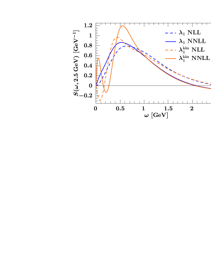
We use the notation $\widehat{\lambda}_{1}$ for a generic short distance definition, which does not suffer from the renormalon ambiguity. Any $\widehat{\lambda}_{1}$ can be related to $\lambda_{1}$ by a perturbative series $\delta\lambda_{1}\sim\alpha_{s}+\alpha_{s}^{2}+\ldots$, where $\widehat{\lambda}_{1}=\lambda_{1}-\delta\lambda_{1}$. For the kinetic scheme the $u=1$ renormalon ambiguity is avoided by defining $\lambda_{1}^{\rm kin}$ using the second moment of a time-ordered product of currents with an explicit hard cutoff regulator $\mu_{f}$ Bigi:1994ga . Here $Z_{1}$ and $\delta\lambda_{1}\propto\mu_{f}^{2}\alpha_{s}$. Since the kinetic energy operator mixes into $\bar{b}_{v}b_{v}$, it modifies the perturbation series multiplying $\bar{b}_{v}b_{v}$, and it is believed that this removes the corresponding $u=1$ infrared renormalon in the Wilson coefficients. In Ref. Bosch:2004th a “shape function” scheme for $\lambda_{1}$ was introduced based on the second moment of $S(\omega,\mu)$ with a cutoff, which also has $\delta\lambda_{1}\propto\mu_{f}^{2}\alpha_{s}$. A potential problem with these schemes is that they resolve an issue with the large-order behavior of perturbation theory by introducing a series that starts with a term $\delta\lambda_{1}\sim\alpha_{s}$. While the inclusion of an $\mathcal{O}(\alpha_{s})$ term is known to provide good numerical stability when removing the $u=1/2$ renormalon from the pole mass, far less numerical analysis has been done on the low-order impact of the $u=1$ renormalon in $\lambda_{1}$. If the low-order series is not yet influenced by the $u=1$ renormalon, then schemes with an $\mathcal{O}(\alpha_{s})$ correction may oversubtract, and not improve the perturbation series. In Fig. 14 we show that in our shape function analysis there is evidence that this is the case. The dashed and solid curves are the NLL and NNLL results, respectively. The curves show $S(\omega,\mu_{i}=2.5\,\mathrm{GeV})$ with the kinetic mass scheme, but use either $\lambda_{1}^{\rm kin}$ (blue curves) or $\lambda_{1}$ from Eq. (123) (orange curves). In the $\lambda_{1}^{\rm kin}$ scheme the oscillatory behavior near the origin at both NLL and NNLL order is indicative of an oversubtraction.

Figure 14: Effect of the short distance subtractions $\delta\lambda_{1}^{\mathrm{kin}}$ for the kinetic scheme at NLL (dashed) and NNLL (solid) on $S(\omega,2.5\,\mathrm{GeV})$ for $\mu_{\Lambda}=1.0\,\mathrm{GeV}$. The blue (dark) lines correspond to using $m_{b}^{\mathrm{kin}}$ together with $\lambda_{1}^{\mathrm{pole}}$, while orange (light) lines use both $m_{b}^{\mathrm{kin}}$ and $\lambda_{1}^{\mathrm{kin}}$.

Some understanding of the weakness of the $u=1$ renormalon can be obtained from analytic computations. For Lorentz invariant regulators the $u=1$ renormalon for $\lambda_{1}$ is “invisible” Martinelli:1995zw ; Neubert:1996zy , namely the ambiguity for $\lambda_{1}$ is smaller than dimensional analysis indicates. In perturbation theory renormalon ambiguities appear as a divergent series with terms $\sim n!\,\alpha_{s}^{n+1}$. However, the leading renormalon series $\sim n!\,\beta_{0}^{n}\alpha_{s}^{n+1}$ is absent, hence the renormalon ambiguity at lowest order in $\lambda_{1}$ is “invisible” Martinelli:1995zw . Correspondingly, at one-loop order $Z_{\rm I}=0$ for Lorentz invariant regulators (even for a hard cutoff), and generically $Z_{1}\propto C_{A}\alpha_{s}^{2}$ Neubert:1996zy . In the kinetic scheme the regulator is not Lorentz invariant, and hence not suppressed by “invisibility”. The same holds for definitions of $\lambda_{1}$ involving a lattice spacing regulator Martinelli:1995zw .

To avoid oversubtractions from $\lambda_{1}$ at low orders in perturbation theory, we would like to define a short distance scheme with $\delta\lambda_{1}\sim\alpha_{s}^{2}$. This can be achieved by finding a scheme that is consistent with the suppression indicated by the invisible renormalon. To construct an “invisible scheme” for $\lambda_{1}$ we define

$$\lambda_{1}^{\mathrm{i}}(R)=\lambda_{1}-\delta\lambda_{1}^{\mathrm{i}}(R)\,,$$ (124)

where the series in $\alpha_{s}$ is obtained by evaluating the matrix element

$$\delta\lambda_{1}^{\mathrm{i}}(R)=\langle b_{v}\lvert\bar{b}_{v}(iD_{\perp})^{2}\,b_{v}\rvert b_{v}\rangle\Big{|}_{R}\,.$$ (125)

Here, $R$ is a Lorentz invariant hard cutoff UV regulator, ensuring that $\delta\lambda_{1}^{\mathrm{i}}(R)\sim R^{2}\alpha_{s}^{2}$. The definition in Eq. (124) states that the invisible scheme $\lambda_{1}^{\mathrm{i}}(R)$ is the kinetic energy of the $b$ quark in the $B$ meson minus the free kinetic energy of the $b$ quark. Since the ${\cal O}(\Lambda_{\rm QCD}^{2})$ ambiguity in $\lambda_{1}$ is a UV effect caused by the mixing of the kinetic operator into $\bar{b}_{v}b_{v}$, it is the same for the $B$ meson and $b$ quark states, and cancels out in the difference. This can be seen explicitly by using Eq. (122) and noting that our states are normalized so that $\langle B_{v}|\bar{b}_{v}b_{v}|B_{v}\rangle=\langle b_{v}|\bar{b}_{v}b_{v}|b_{v}\rangle=1$. The ${\cal O}(\Lambda_{\rm QCD}^{2})$ ambiguity is universal to the definition of $\lambda_{1}$ and independent of $R$. Although a precise definition of $R$ is needed to define the scheme, the $u=1$ renormalon ambiguity cancels out in $\lambda_{1}-\delta\lambda_{1}^{\mathrm{i}}$ for any such regulator. We adopt a definition that allows us to use the computation in Ref. Neubert:1996zy , where it was shown that $Z_{1}\neq 0$ at ${\cal O}(\alpha_{s}^{2})$ in a Lorentz invariant cutoff scheme. We define

$$\delta\lambda_{1}^{\mathrm{i}}(R) =\lim_{v^{\prime}\to v}A_{vv^{\prime}}(0,0)\Big{|}_{R}$$ (126)

$$=\lim_{v^{\prime}\to v}\int_{0}^{R}\!\int_{0}^{R}\!\frac{\mathrm{d}w\,\mathrm{d}w^{\prime}}{(2\pi i)^{2}\,w\,w^{\prime}}\,\mbox{\raisebox{-7.0pt}{$\stackrel{{\scriptstyle\displaystyle\rm Disc}}{{w}}$}}\,\mbox{\raisebox{-9.5pt}{$\stackrel{{\scriptstyle\displaystyle\rm Disc}}{{w^{\prime}}}$}}\,A_{vv^{\prime}}(w,w^{\prime})\,,$$

where

$$A_{vv^{\prime}}(v\cdot k,v^{\prime}\cdot k^{\prime})=\frac{3\,\langle b_{v^{\prime}}(k^{\prime})\lvert\bar{b}_{v^{\prime}}v_{\mu}v^{\prime}_{\nu}\,ig\,G^{\mu\nu}b_{v}\rvert b_{v}(k)\rangle}{(v\cdot v^{\prime})^{2}-1}\,,$$ (127)

and as usual the discontinuity of a function is given by ${\rm Disc}_{w}\,f(w)=\lim_{\epsilon\to 0}\big{[}f(w+i\epsilon)-f(w-i\epsilon)\big{]}$. Note that it is sufficient to consider the $\bar{b}_{v^{\prime}}ig\,G^{\mu\nu}b_{v}$ operator due to the virial theorem in HQET, which relates $\lim_{v^{\prime}\to v}A_{vv^{\prime}}(0,0)$ to the corresponding matrix element of the kinetic energy operator in Eq. (125). The result for the cutoff matrix element from Ref. Neubert:1996zy implies

$$\delta\lambda_{1}^{\mathrm{i}}(R) =R^{2}\,C_{F}C_{A}\biggl{(}\frac{\pi^{2}}{3}-1\biggr{)}\,\frac{\alpha_{s}^{2}(\mu)}{4\pi^{2}}$$

$$=0.232\,R^{2}\,\alpha_{s}^{2}(\mu)\,.$$ (128)

Equation (C) gives the relation of the invisible $\lambda_{1}^{\mathrm{i}}$ to the HQET $\lambda_{1}$ in Eq. (123), which was used in the text. We use $R=1\,\mathrm{GeV}$ as our default value. Equations (124) and (126) provide a $\mu$ independent definition for $\lambda_{1}^{\mathrm{i}}(R)$, so the $\mu$ dependence in $\alpha_{s}^{2}(\mu)$ will cancel against a higher order $R^{2}\alpha_{s}^{3}(\mu)\ln(\mu/R)$ term in $\delta\lambda_{1}^{\mathrm{i}}(R)$.

References

- (1) M. Neubert, Phys. Rev. D 49 (1994) 3392 [hep-ph/9311325]; ibid. 4623 [hep-ph/9312311].
- (2) I. I. Y. Bigi, M. A. Shifman, N. G. Uraltsev and A. I. Vainshtein, Int. J. Mod. Phys. A 9 (1994) 2467 [hep-ph/9312359].
- (3) K. S. M. Lee, Z. Ligeti, I. W. Stewart and F. J. Tackmann, Phys. Rev. D 74, 011501(R) (2006) [hep-ph/0512191];
- (4) K. S. M. Lee and I. W. Stewart, Phys. Rev. D 74, 014005 (2006) [hep-ph/0511334].
- (5) M. Misiak et al., Phys. Rev. Lett. 98, 022002 (2007) [hep-ph/0609232]; and references therein.
- (6) S. Chen et al. [CLEO Collaboration], Phys. Rev. Lett. 87, 251807 (2001) [hep-ex/0108032].
- (7) K. Abe et al. [Belle Collaboration], arXiv:0804.1580; P. Koppenburg et al. [Belle Collaboration], Phys. Rev. Lett. 93, 061803 (2004) [hep-ex/0403004].
- (8) B. Aubert et al. [BABAR Collaboration], Phys. Rev. D 77, 051103(R) (2008) [arXiv:0711.4889]; Phys. Rev. Lett. 97, 171803 (2006) [hep-ex/0607071]; Phys. Rev. D 72, 052004 (2005) [hep-ex/0508004].
- (9) B. Aubert et al. [BABAR Collaboration], hep-ex/0408068; K. Tackmann [BABAR Collaboration], arXiv:0801.2985.
- (10) C. W. Bauer, Z. Ligeti, M. Luke, A. V. Manohar and M. Trott, Phys. Rev. D 70, 094017 (2004) [hep-ph/0408002]; C. W. Bauer, Z. Ligeti, M. Luke and A. V. Manohar, Phys. Rev. D 67, 054012 (2003) [hep-ph/0210027].
- (11) O. Buchmüller and H. Flächer, Phys. Rev. D 73, 073008 (2006) [hep-ph/0507253].
- (12) E. Barberio et al. [Heavy Flavor Averaging Group], arXiv:0704.3575; and updates at http://www.slac.stanford.edu/xorg/hfag/.
- (13) C. Balzereit, T. Mannel and W. Kilian, Phys. Rev. D 58, 114029 (1998) [hep-ph/9805297].
- (14) S. W. Bosch, B. O. Lange, M. Neubert and G. Paz, Nucl. Phys. B 699, 335 (2004) [hep-ph/0402094].
- (15) A. K. Leibovich, I. Low and I. Z. Rothstein, Phys. Rev. D 61, 053006 (2000) [hep-ph/9909404].
- (16) A. K. Leibovich, I. Low and I. Z. Rothstein, Phys. Lett. B 486, 86 (2000) [hep-ph/0005124].
- (17) A. H. Hoang, Z. Ligeti and M. Luke, Phys. Rev. D 71, 093007 (2005) [hep-ph/0502134].
- (18) B. O. Lange, JHEP 0601, 104 (2006) [hep-ph/0511098].
- (19) C. W. Bauer, Z. Ligeti and M. E. Luke, Phys. Lett. B 479 (2000) 395 [hep-ph/0002161]; Phys. Rev. D 64 (2001) 113004 [hep-ph/0107074].
- (20) A. H. Hoang and I. W. Stewart, Phys. Lett. B 660, 483 (2008) [arXiv:0709.3519].
- (21) C. W. Bauer and A. V. Manohar, Phys. Rev. D 70, 034024 (2004) [hep-ph/0312109].
- (22) M. Neubert, Eur. Phys. J. C 40, 165 (2005) [hep-ph/0408179].
- (23) T. Becher and M. Neubert, Phys. Rev. Lett. 98, 022003 (2007) [hep-ph/0610067].
- (24) G. P. Korchemsky and G. Sterman, Phys. Lett. B 340, 96 (1994) [hep-ph/9407344];
- (25) C. W. Bauer, D. Pirjol and I. W. Stewart, Phys. Rev. D 65, 054022 (2002) [hep-ph/0109045].
- (26) T. Mannel and F. J. Tackmann, Phys. Rev. D 71, 034017 (2005) [hep-ph/0408273].
- (27) F. J. Tackmann, Phys. Rev. D 72, 034036 (2005) [hep-ph/0503095].
- (28) B. O. Lange, M. Neubert and G. Paz, Phys. Rev. D 72, 073006 (2005) [hep-ph/0504071].
- (29) W. M. Yao et al. [Particle Data Group], J. Phys. G 33, 1 (2006), and 2007 partial update for the 2008 edition.
- (30) A. H. Hoang, Z. Ligeti and A. V. Manohar, Phys. Rev. Lett. 82 (1999) 277 [hep-ph/9809423]; Phys. Rev. D 59 (1999) 074017 [hep-ph/9811239]; A. H. Hoang and T. Teubner, Phys. Rev. D 60 (1999) 114027 [hep-ph/9904468].
- (31) A. Czarnecki, K. Melnikov and N. Uraltsev, Phys. Rev. Lett. 80, 3189 (1998) [hep-ph/9708372]; Phys. Rev. D 57, 1769 (1998) [hep-ph/9706311]; the part of what later became was first obtained in: A. Kapustin, Z. Ligeti, M. B. Wise and B. Grinstein, Phys. Lett. B 375, 327 (1996) [hep-ph/9602262].
- (32) S. Fleming, A. H. Hoang, S. Mantry and I. W. Stewart, Phys. Rev. D 77, 114003 (2008) [arXiv:0711.2079].
- (33) F. De Fazio and M. Neubert, JHEP 9906, 017 (1999) [hep-ph/9905351].
- (34) P. Gambino, P. Giordano, G. Ossola and N. Uraltsev, JHEP 0710, 058 (2007) [arXiv:0707.2493].
- (35) M. Abramowitz and I. A. Stegun, “Handbook of Mathematical Functions”, Dover, New York (1964); for other proposed expansions, see, e.g.: A. H. Hoang and R. Hofmann, Phys. Rev. D 67, 054024 (2003) [hep-ph/0206201].
- (36) C. W. Bauer, M. E. Luke and T. Mannel, Phys. Rev. D 68, 094001 (2003) [hep-ph/0102089].
- (37) A. K. Leibovich, Z. Ligeti and M. B. Wise, Phys. Lett. B 539, 242 (2002) [hep-ph/0205148].
- (38) C. W. Bauer, M. Luke and T. Mannel, Phys. Lett. B 543, 261 (2002) [hep-ph/0205150].
- (39) K. S. M. Lee and I. W. Stewart, Nucl. Phys. B 721, 325 (2005) [hep-ph/0409045].
- (40) A. Kapustin, Z. Ligeti and H. D. Politzer, Phys. Lett. B 357, 653 (1995) [hep-ph/9507248].
- (41) S. J. Lee, M. Neubert and G. Paz, Phys. Rev. D 75, 114005 (2007) [hep-ph/0609224].
- (42) K. S. M. Lee, Phys. Rev. D 78, 013002 (2008) [arXiv:0802.0873].
- (43) M. Beneke, F. Campanario, T. Mannel and B. D. Pecjak, JHEP 0506, 071 (2005) [hep-ph/0411395].
- (44) M. Trott and A. R. Williamson, Phys. Rev. D 74, 034011 (2006) [hep-ph/0510203].
- (45) J. R. Andersen and E. Gardi, JHEP 0601, 097 (2006) [hep-ph/0509360].
- (46) U. Aglietti, F. Di Lodovico, G. Ferrera and G. Ricciardi, arXiv:0711.0860.
- (47) M. Neubert, Phys. Rev. D 72, 074025 (2005) [hep-ph/0506245].
- (48) K. S. M. Lee, Z. Ligeti, I. W. Stewart and F. J. Tackmann, Phys. Rev. D 75, 034016 (2007) [hep-ph/0612156];
- (49) K. G. Chetyrkin, M. Misiak and M. Münz, Phys. Lett. B 400, 206 (1997) [Erratum-ibid. B 425, 414 (1998)] [hep-ph/9612313].
- (50) C. W. Bauer, S. Fleming, D. Pirjol and I. W. Stewart, Phys. Rev. D 63, 114020 (2001) [hep-ph/0011336].
- (51) I. R. Blokland, A. Czarnecki, M. Misiak, M. Slusarczyk and F. Tkachov, Phys. Rev. D 72, 033014 (2005) [hep-ph/0506055]; K. Melnikov and A. Mitov, Phys. Lett. B 620, 69 (2005) [hep-ph/0505097].
- (52) A. Ali, B. D. Pecjak and C. Greub, Eur. Phys. J. C 55, 577 (2008) [arXiv:0709.4422].
- (53) T. Becher and M. Neubert, Phys. Lett. B 637, 251 (2006) [hep-ph/0603140].
- (54) T. Becher and M. Neubert, Phys. Lett. B 633, 739 (2006) [hep-ph/0512208].
- (55) G. P. Korchemsky and A. V. Radyushkin, Nucl. Phys. B 283, 342 (1987).
- (56) S. Moch, J. A. M. Vermaseren and A. Vogt, Nucl. Phys. B 688, 101 (2004) [hep-ph/0403192].
- (57) G. P. Korchemsky and G. Marchesini, Nucl. Phys. B 406, 225 (1993) [hep-ph/9210281].
- (58) E. Gardi, JHEP 0502, 053 (2005) [hep-ph/0501257].
- (59) A. Jain, I. Scimemi and I. W. Stewart, Phys. Rev. D 77, 094008 (2008) [arXiv:0801.0743].
- (60) G. Martinelli, M. Neubert and C. T. Sachrajda, Nucl. Phys. B 461, 238 (1996) [hep-ph/9504217].
- (61) M. Neubert, Phys. Lett. B 393, 110 (1997) [hep-ph/9610471].
- (62) M. E. Luke and A. V. Manohar, Phys. Lett. B 286, 348 (1992) [hep-ph/9205228].
- (63) M. Beneke, V. M. Braun and V. I. Zakharov, Phys. Rev. Lett. 73, 3058 (1994) [hep-ph/9405304]; M. E. Luke, A. V. Manohar and M. J. Savage, Phys. Rev. D 51, 4924 (1995) [hep-ph/9407407]; M. Neubert and C. T. Sachrajda, Nucl. Phys. B 438, 235 (1995) [hep-ph/9407394].
- (64) I. I. Y. Bigi, M. A. Shifman, N. G. Uraltsev and A. I. Vainshtein, Phys. Rev. D 52, 196 (1995) [hep-ph/9405410].