Numerical study of ground state energy fluctuations in spin glasses
Abstract
Using a stochastic algorithm introduced in a previous paper, we study the finite size volume corrections and the fluctuations of the ground state energy in the Sherrington-Kirkpatrick and the Edwards-Anderson models at zero temperature. The algorithm is based on a suitable annealing procedure coupled with a balanced greedy-reluctant strategy that drives the systems towards the deepest minimum of the energy function.
1 Introduction
Finding solutions of computationally hard problems is an outstanding issue in applied science. A classical example of hard problem is the search of the optimal configurations of a functional with many local minima and a complex landscape: in fact, in this case the solution is usually achieved with a computational effort that increases exponentially with the dimension of the problem. Typically, such functionals arise in the modelling of competing interactions among the components of large system. In some interesting cases in physics and in other field (for example in biology, in economy, in computer sciences,…), the interactions depend on some frozen-in structural disorder [1], and any realization of the disorder defines a sample of the system. Obviously, the thermodynamic properties of such systems, like spin glasses, fluctuate from sample to sample. Indeed, the statistical variables of the system (spins, in the case of spin glasses) interact via some random potential which models the quenched disorder. In this paper we consider the fluctuations, with respect to disorder realizations, of the low-lying states energy of spin glasses (thus the functional to be optimized here is the energy of the configurations of spins). Disorder-induced fluctuations are particularly relevant for the physics of systems at low temperatures. In fact, the properties of such systems are largely dominated by the states with minimal energy into which the Gibbs-Boltzmann distribution collapses as the temperature is decreased.
In order to be more specific, let us consider a disordered model with finite volume and described by a Hamiltonian (or energy function) which depends on a set of statistical variables (the degrees of freedom of the system) and on a set of variables , representing the quenched disorder of the system, which are randomly sampled according to a given probability distribution. For a fixed disorder realization and at zero temperature, the relevant states of the system are only the ground states, that is the configurations whose energy (for degree of freedom) is given by . Being the minimum of a set of random variables, the energy density is also a random variable whose probability density function (PDF) follows some (a priori unknown) extreme values statistics: we are interested in the numerical study of this distribution in its large volume limit. In particular, we will mainly focus on the mean value and on the standard deviation (here represents the average with respect to disorder), but we will also try to give some insight into the shape of . In order to study their scaling behavior, we assume that and have a definite limit as goes to infinity: and ; in other words we suppose that extensivity and self-averaging of the energy density hold (these properties are, in fact, satisfied in the models that we are going to study). More precisely, assuming a power-law scaling behavior for the relevant quantities:
| (1) |
we aim at estimating the exponents and .
Since extensivity and self-averaging imply a trivial distribution in the large volume limit (), we inquire into the scaling behavior of (if any) by studying the centered and scaled variable and seeking for its distribution in the infinite volume limit.
The previous issues have been numerically addressed by several authors in recent years [2, 3] and a variety of spin glasses models have been considered [4, 5, 6]. All these studies call for large computational resources. Indeed, the computational effort required to solve the intrinsically complex problem of finding the ground state of [1], has to be multiplied by the large number of realizations requested in the computation of the disorder averages over systems with larger and larger volumes. In the cited papers [2]-[6] many different techniques are employed in the approximation of the ground state. Indeed, the relevance of solving intrinsically complex problems, has prompted many authors to devise efficient algorithms implementing many different approaches to this issue. In this study we rely on a stochastic algorithm, inspired by the classical simulated annealing technique, which was introduced in [7]. In that paper the algorithm was challenged against the search of the ground state in the Sherrington-Kirkpatrick model (SK), which has become the standard of NP-complete problems. Our purpose here is to push forward the validation of the algorithm by studying in some details the probability distribution . Moreover, forcing the scope of the algorithm that was optimized in [7] for SK, we extend the study to a preliminary analysis of the ground state of Edwards-Anderson model (EA). All the results that we are going to describe are completely consistent with ones already present in the literature.
The paper is organized as follows. In section 2 we introduce the spin glasses studied in this work, namely the Sherrington-Kirkpatrick and the Edwards-Anderson models, and review briefly some theoretical results that are relevant to the present issues. We sketch the algorithm in section 3, referring to the original paper for details. The results are given in sections 4.
2 The models
The Ising spin glass models we study are the Sherrington-Kirkpatrick model (SK) [8], whose Hamiltonian is defined by
| (2) |
and the Edwards-Anderson model (EA) [9], whose the Hamiltonian is
| (3) |
where for are Ising spin variables which interact through couplings . For both models, are independent identically distributed gaussian random variables, with zero mean and variance for SK and for EA. With this choice of the variance the extensivity and self-averaging of the ground state energy density of the two models are guaranteed.
For three dimensional EA, which is a short range spin glass model, the sum in (3) is over nearest neighbor spins on a given square or cubic lattice of linear size (thus the number of nodes is , where is the dimension of the lattice), while for SK, which is the mean field approximation of EA, the sum is over all the spins. (For the physical origin of these models and a general overview on spin glass, see [10])
The SK model in the low temperature phase was solved through the replica symmetry breaking ansatz (RSB) by G. Parisi [1]. This solution, which is universally believed to be true for SK, is still a debated issue in the mathematical physics community, because rigorous proofs of some fundamental properties of the RSB scenario (for instance ultrametricity [1]) are lacking. However, recently some progress has been done in this direction with the mathematical proof of the Parisi formula for the free energy density [11, 12]. In the framework of the RSB theory, the knowledge of the ground state energy in the thermodynamic limit ( [1]) and the probability distribution of large deviations of the free energy at all temperatures [13] are available, but there are no exact analytic results for the limiting behavior of the PDF. A computation performed at the critical temperature and at the de Almeida-Thouless line in [14], gives a scaling exponent of the internal energy density equal to . In a more recent paper [15] a heuristic argument is presented which leads the same value just below . It is natural to extrapolate this result to zero temperature obtaining for the ground state energy density . Indeed in [15] the authors argue, on the basis of the numerical evidence, that this should be the scaling exponent in the whole spin glass phase. Similarly, there are no analytical calculations for the sample-to-sample fluctuation exponent of the internal energy at zero temperature. However, different analytical estimates for the fluctuation exponent of the free energy density are available: [13, 15, 16] or [17]. As in the case of , we can expect the exponent to be the same as that for the free energy density in the whole region below [2], and in particular at zero temperature. Unfortunately, given the closeness of the predicted values, any numerical test at zero as well as at finite temperature can hardly provide a sharp distinction between two possibilities.
For the Edwards Anderson model things are even messier because there is not a general consensus on the nature of its low temperature phase, and several scenarios (besides RSB) are conflicting [18]. Regarding our concern, a relevant result was proven by Wehr and Aizenman [19]: they proved that for EA, as for any finite-range spin glass model in finite dimension , the scaling exponent for the standard deviation is , namely that the ground-state energy variance grows linearly with the volume . In fact, in [19] it is shown that the variance of any extensive quantity depending on random parameters is of the order of the volume . Even if this result seems to suggest a gaussian limiting behavior for , the authors of [19] state that this, in general, should be false, though only very mild violations to the normal distribution are to be expected. However, for EA, heuristic arguments as well as numerical evidence point to a gaussian limit for [2]. The same distribution and the same estimate have been obtained by Aspelmeier and Moore with a replica theory calculation in [20].
3 The algorithm
The numerical approach to the questions presented in Sec.1 requires the computation of the minima of for a large sample of disorder realizations, that is the search for the spin configuration which minimizes the energy (ground state configuration). The minimization of a certain function depending on many discrete variables (Hamiltonian) is a combinatorial optimization problem. Since often many combinatorial optimization problems are NP complete, they are tackled by constructing approximation algorithms, that run in acceptable amounts of computational time and have the property that final configurations are “close” to globally minimal ones (the metastable states approximate the ground state). The models we consider are often presented as the standard example of NP-problems. Indeed, the random sign (and strength) of the interaction generates frustration in the systems, i.e. the fact that in low energy configurations some of the couples will have unsatisfied interaction. Therefore, the global minimization can not be achieved simply by minimizing each local spin-to-spin interaction. As a consequence, the ground state of the systems is far from the standard ground state of ferromagnetic models, where all spins point in the same direction.
Several numerical studies have tried different algorithms in the search of ground-state energies, for example gradient descendent [21, 22, 23], simulated annealing [24, 25], genetic algorithms [2, 3], branch-and-bound algorithm [26] and extremal optimization [4, 27, 28]. In this paper we use a stochastic algorithm which is the optimal one in a class introduced in [7]. The algorithm is required to reach the lowest possible minima as quickly as possible avoiding to get stuck in a local minimum which is still far from the deepest ones. In fact, in these complex systems disorder and frustration produce an energy function with a corrugated landscape, with a high multiplicity of valleys (local minima) separated by high barriers (local maxima).
Our algorithm generates a one spin-flip dynamics in the configuration space; indeed, starting from a randomly chosen initial condition, the algorithm explores the space through a sequence of configurations obtained by inverting a single spin sign to pass from a spin configuration to successive one. The stochastic transition from a trajectory point to another is ruled by a probability with an exponential density.
Essentially, the idea is that at each step one generates a priori a random energy jump (variation) with probability and then one moves in the direction that produces the nearest energy variation to the chosen jump. The algorithm stops in a local minimum that represents the best (sufficiently deep) encountered minimum. This algorithm is justified by statistical properties of the metastable states: these states are organized with a certain structure so that the dynamic evolution can be considered as the overlapping of a fast motion in the attraction basin of a local minimum and of a slow one with possibility of jumps between minima. The possibility of exceed the energy barriers, needed to escape from poor local minima, is obtained by introducing a sort of “external temperature” in the system, which enables random positive energy fluctuations. The energy transitions are generated in accordance with the following PDF
in which the control parameter is mainly represented by the cooling rate of the system and is the time of the dynamics, i.e. the number of spin-flips since the beginning of the algorithm execution. The choice of the exponential distribution is standard in statistical mechanics and reflects the Gibbs-Boltzmann equilibrium ensemble. The probability of energy increasing jumps is given by , with increasing in . This strategy is designed to model an initially hot system ( small) with high probability of positive moves, which is gradually quenched (the higher the temperature, the more likely are moves upwards and viceversa); when the system is cool ( large), positive fluctuations are absent and the decreasing trajectories are forced to follow greedy-like paths (very large jumps deep into a valley). With this type of algorithm we try to take advantage during the paths both of the greedy-like behavior and of the reluctant one (very small jumps and slow convergence). Obviously the performance of the algorithm in terms of lowest energy found and execution time, depends on the choice of the optimal cooling rate . In [7] the cooling rate, with an exponential dependence on the time , was optimized for the SK model.
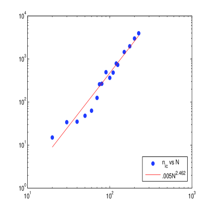
The large statistics of ground state values required by our analysis is obtained as follows. For a fixed disorder realization , we performed independent runs of the algorithm. Each run starts from an initial condition drawn at random from the uniform distribution. The (approximate) ground state energy is then obtained as the lowest energy of the metastable states sampled along the trajectories. With the above strategy, the computed depends, in principle, on . Therefore, the reliability of the results can be tested, in a self consistent way, by computing the lowest energy from larger and larger sets of initial conditions and by measuring the number of runs needed to stabilize the value within a given accuracy . This stabilized value is assumed to be the ground state energy for the given realization of the model. In the case of SK, for instance, running the algorithm with the optimal cooling rate [7], the dependence of on the volume is for (see Fig.1). The linear system sizes, the number of initial conditions and the number of disorder realizations used in our simulations are reported in Tab. 1 for both SK and EA model.
| 50 | 50 | ||
| 75 | 300 | ||
| SK | 100 | 500 | |
| 150 | |||
| 200 | |||
| 3-4 | 200 | ||
| 5 | 200 | ||
| 6 | |||
| EA2D | 7 | ||
| 8-9 | |||
| 10 | |||
| 11 | |||
| 3-4 | |||
| EA3D | 5 | ||
| 6 |
4 Results
We tested the power law (1) for the mean ground state energy density of the SK model, sampling different system volumes between and , with from up to disorder realizations each (see Tab. 1). These values of have been considered appropriate because of the (relatively) fast convergence of the sample mean of ’s to its limit value, as is increased.
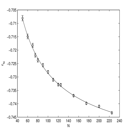
Fitting the data to the power law with three free parameters, we obtain the values . The influence of the subleading corrections neglected in (1) can be appreciated by restricting the fit to larger values of . Indeed, with we have: , (see Fig. 2). In both cases, the estimated value of is in good agreement with Parisi’s analytical value [1]. The scaling exponent has been computed in previous numerical studies by Palassini [3], Bouchaud et al. [2], Katzgraber and Campbell [29]; all these results suggest . Our estimate of with is compatible with this value, even though the uncertainty on the data are much larger than those presented in [2]. On the other hand, the error on the exponent can be lowered by fitting the data with only two free parameters and letting ; in doing so, we obtain (for ) and for . Moreover, fixing also we obtain for and for . Let us conclude this point by observing that the previous estimates of are quite close to the value of obtained in [15] fitting to the values of the internal energy at . In [15] the power law has been found to describe closely the data in the whole spin glass phase.
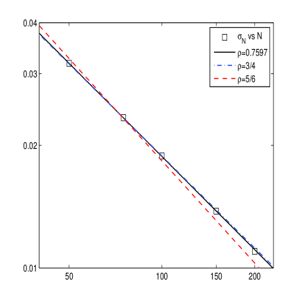
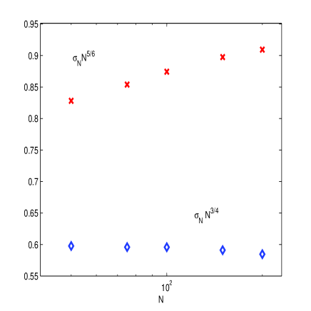
In Fig. 3 we represent in log-log scale the numerical data for as a function of together with the best numerical fit , which gives . As already said in the introduction, in literature two values are conjectured for the scaling exponent of the sample to sample fluctuations: and [2, 3, 17, 22]. As it is apparent from Figg. 3 and 4, the exponent (blue line) is consistent with our data, while seems to be less likely to occur (red line in Fig. 3 and red crosses in Fig. 4). This is in agreement with the results in literature in which all the estimates are smaller than . In particular, the value was obtained in [3] and later confirmed in [2], but while in the former paper is ruled out, the authors of the latter can not draw the same conclusion. A similar uncertainty is present also in simulations at finite temperature; indeed, in [15] at the data for the internal energy are compatible with but is not ruled out. The value is supported also by some recent theoretical results [13, 15] suggesting that the sample-to-sample fluctuations should be proportional to .
The detection of the distribution for large is obviously much more difficult than studying the two moments and . Such a study has been addressed in [2, 3, 15] via numerical simulations; here we will give some insight into this issue following closely the approach of [3]. The problem pertains to the statistics of extremes; in this theory the scaling of the minimum of a family of random variables is studied for large . Here the random variables are the energies of the spin configurations , the minimum is the ground state energy , and the scaling is studied using the variables . In the quoted papers the data are tested against the standard extreme values distributions of a family of identically distributed (i.i.d.) random variables: 1) Gumbel, if the individual distribution of the random variables is unbounded and decreases faster than any power law; 2) Fisher, if the distribution decreases as a power law; 3)Weibull, if the distribution has a cut-off. In the papers [2, 3] it is shown that none of the previous distributions describe the data. The same negative result was obtained [3, 15] testing the Tracey-Widom distribution for correlated variable. While it is not unexpected the failure of the Gumbel distribution in describing the data (since the energy levels that contribute to the ground state energy for the mean field SK model are not independent), it is much more surprising that the approximate behavior of the data can be found in the family of the generalized Gumbel distributions. These are the distributions the -th smallest value in a set of i.i.d. random variables [30]
where , and are constant parameter. In his paper [3] Palassini found that the Gumbel distribution with describes quite closely the ground state energy distribution of SK; our data support this statement. In Fig. 6 and 6 the empirical distributions of for the volumes , are reported together with and the standard normal distribution. The values of parameters in , taken from [3], are chosen imposing zero mean and unit variance. Even if the data for the larger sizes, see Fig.6, are much more noisy than those for the smaller ones, the agreement with seems fairly clear for all the sizes. A further support can be obtained by comparing the curtosis and the skewness of with the same cumulants of the variable at different sizes, see table 2.
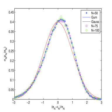
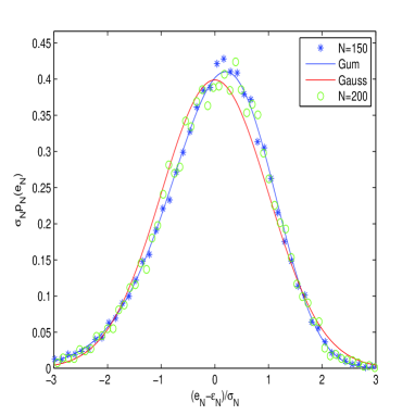
| Kurtosis | Skewness | |
|---|---|---|
| 50 | 3.4249 | -.4451 |
| 75 | 3.3148 | -.4052 |
| 100 | 3.3464 | -.4046 |
| 150 | 3.5515 | -.4346 |
| 200 | 3.3312 | -.3599 |
| 3.3535 | -.4247 |
The second family of spin system we study is the Edwards-Anderson model. As we said in the introduction, this should be considered as a preliminary study of the behavior of the algorithm in exploring the low energy configurations of the finite dimensional spin glass model. Indeed, we use the cooling rate optimized for the SK model, both for the two-dimensional and three dimensional cases (square and cubic lattices of linear size ). However, while in the three dimensional case the problem of finding the ground states is NP-hard, the two dimensional one is polynomial [31]. For this reason the three dimensional case is only partially studied, i.e. only small linear sizes are considered.
Nevertheless, our data for -model confirm the results present in the literature [2]. All the parameters used in the numerical simulations both for two dimensional and three dimensional EA model are listed in Tab. 1.
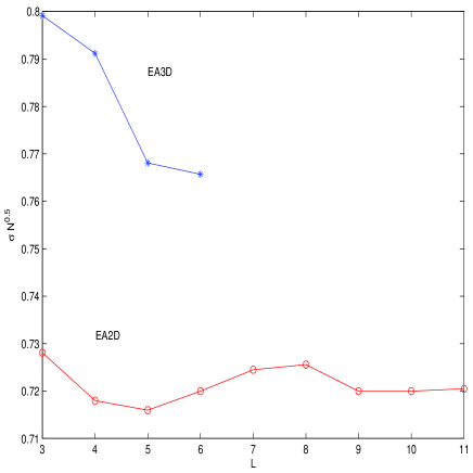
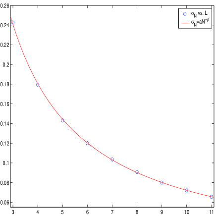
In order to validate our numerical experiment, it is useful to compare the numerical data for with the theoretical prediction . In Fig. 7 we show ; while for our data are compatible with size independence, for a first sketchy study seems to show no analogous trend. In Fig. 8 we represent (for ) the best numerical fit which gives (and ) in accordance with the expected value. This confirms the validity of our algorithm and the consistency of our numerical results for this model. Such a scaling low is expected for the central limit theorem in the cases in which the different terms contributing to the ground-state energy are independent. As a matter of fact, for EA model these terms are correlated; so this type of scaling reads as an indication of weak correlation. In contrast, for SK model, the variables that play a role in the ground state energy are sufficiently correlated to prevent the central limit theorem behavior.
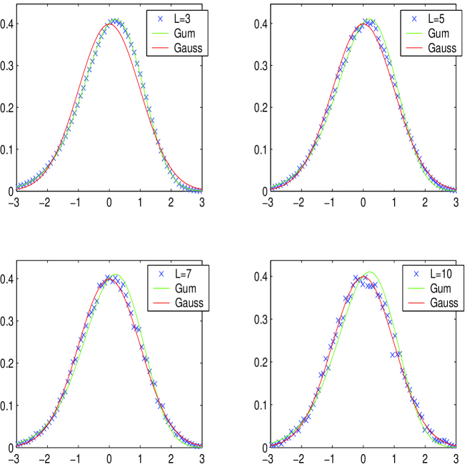
A further support to the hypothesis of weak correlation comes from the study of the limiting shape of the distribution . Because of the dependence of the random variables , we can not have a Gaussian shape for at large (see for example [19]), even though a weakly Gaussian-like behavior is expected (it follows from the Brout’s heuristic argument [10] and also from replica theory calculations [20]). In fact, in the case of the two dimensional lattice, the numerical data for small volumes show that the PDF follows the same Gumbel distribution (with ) already found as the limiting behavior of the SK model. However, as is increased, we observe that the distribution moves away from the Gumbel and seems to approach a Gaussian limiting shape (see Fig. 9).
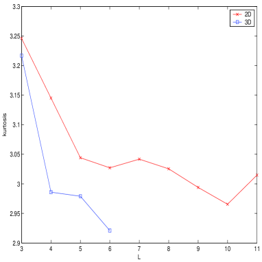
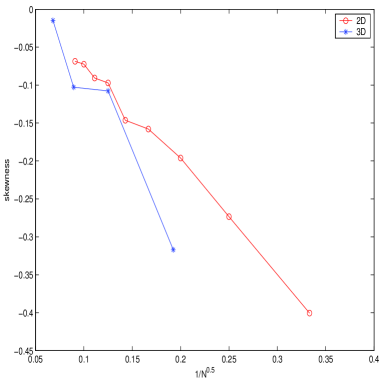
If we consider the kurtosis and the skewness of we have that they decay with the system size (Fig. 11 and 11). The data in Fig. 11 suggest zero limiting values as in accordance with the central limit theorem law that predicts that the skewness scales as (in Fig. 11 the data are completely compatible with a linear convergence to zero, confirming a central limit-like scaling).
Now we move to the study of the finite-size corrections to the mean energy density which, to the leading order, are expected to scale as . For EA model the analytic knowledge of in the thermodynamic limit is not available (unlike in the case of SK model). First we consider the case . We fit our data () to Eq. 1 where , and are free parameters. We obtain (Fig. 12): , and in accordance with [2] that provides .
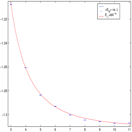
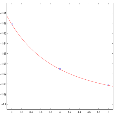
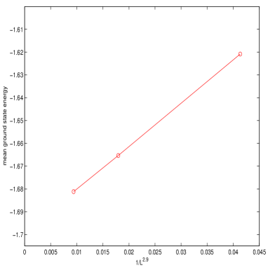
For the best fit gives a mean (intensive) ground state energy decaying as (see Fig 14). In [2] the estimated value of is , even though, due to the uncertainty on the data, any value between and seems possible. In order to check the consistency of our data with this value we compute the linear fit , represented in Fig. 14, which gives , , in good agreement with the values presented in [2].
To conclude, we presented a numerical investigations on mean field and finite-dimensional spin glass models that produce finite size scaling exponents consistent with the results of many works on the subject, but produced with different algorithms. The study of the probability distribution of the ground state energy showed that in the large volume limit it becomes Gaussian for the EA model, but with a finite size behavior close to a Gumbel distribution which, on the other hand, is the limiting distribution for the SK model. Further effort is necessary to produce the optimal algorithm in searching for the ground state of the three-dimensional EA model.
Acknowledgments. We thank Cristian Giardinà and Pierluigi Contucci for many useful discussions that stimulated and improved this work.
References
- [1] M. Mézard, G. Parisi, and M. A. Virasoro, Spin glass theory and beyond, (World Scientific, Singapore, 1987).
- [2] J.-P. Bouchaud, F. Krzakala, and O. C. Martin, Energy exponents and corrections to scaling in Ising spin glasses, Phys. Rev. B 68 (2003) 224404.
- [3] M. Palassini, Ground-state energy fluctuations in the Sherrington-Kirkpatrick model, cond-mat/0307713.
- [4] S. Boettcher, Extremal Optimization for the Sherrington-Kirkpatrick spin glass, Eur. Phys. J. B 46 (2005) 501–505.
- [5] S. Boettcher, Numerical results for ground states of spin glasses on Bethe lattices, Eur. Phys. J. B 31 (2003) 29–39.
- [6] F. Liers, M. Palassini, A. K. Hartmann, and M. Juenger, Ground state of the Bethe lattice spin glass and running time of an exact optimization algorithm, Phys. Rev. B 68 (2003), 094406.
- [7] P.Contucci, C. Giardinà, C. Giberti and C. Vernia, Finding Minima in Complex Landscapes: Annealed, Greedy and Reluctant Algorithms Math. Models Methods Appl. Sci 15 (2005) 1349-1369.
- [8] D. Sherrington and S. Kirkpatrick, Solvable model of a spin-glass, Phys. Rev. Lett. 35 (1975) 1792–1796.
- [9] S. F. Edwards and P. W. Anderson, Theory of spin glasses, J. Phys. F 5 (1975) 965–974.
- [10] K. Binder and A.P. Young, Spin glasses: Experimental facts, theoretical concepts and open questions, Rev. Mod. Phys. 58 (1986) 801–976.
- [11] F. Guerra, Broken replica symmetry bounds in the mean field spin glass model, Comm. Math. Phys. 233 (2003) 1–12.
- [12] M. Talagrand, The Parisi formula, Ann. Math. 163 (2006) 221–263.
- [13] G. Parisi, T. Rizzo, Large deviations in the free-energy of mean-field spin-glasses, (2007) http://arxiv.org/abs/0706.1180v1.
- [14] G. Parisi, F. Ritort, F. Slanina, Several results on finite-size corrections in the Sherrington-Kirkpatrick spin-glass model, J. Phys. A 26 (1993) 3775–3789.
- [15] T. Aspelmeier, A. Billoire, E. Marinari, M.A. Moore, Finite size corrections in the Sherrington-Kirkpatric model http://arxiv.org/0711.3445v1.
- [16] A. Crisanti, G. Paladin, J.-J. Sommers, A. Vulpiani, Replica trick and fluctuations in disordered systems, J. Phys. I 2 (1992) 1325–1332.
- [17] T. Aspelmeier, M.A. Moore, A.P. Young, Interface Energies in Ising Spin Glasses, Phys. Rev. Lett. 90 (2003) 127202.
- [18] C.M. Newman and D.L. Stein, Order and broken symmetry in short-ranged spin glasses, J. Phys: Condens. Matter 15 (2003) R1319–R1364.
- [19] J. Wehr and M. Aizenman, Fluctuations of Extensive Functions of Quenched Random Couplings, J. Stat. Phys. 60 (1990) 287–306.
- [20] T. Aspelmeier and M. Moore, Free Energy Fluctuations in Ising Spin Glasses, Phys. Rev. Lett. 90 (2003) 177201.
- [21] F. T. Bantilan and R. G. Palmer, Magnetic properties of a model spin glass and the failure of linear response theory, J. Phys. F 11 (1981) 261–266.
- [22] S. Cabasino, E. Marinari, P. Paolucci and G. Parisi, Eigenstates and limit cycles in the SK model, J. Phys. A: Math. Gen. 21 (1988) 4201–4210.
- [23] P.Contucci, C. Giardinà, C. Giberti, F. Unguendoli and C. Vernia, Interpolating greedy and reluctant algorithms, Optim. Methods Softw. 20, (2005), 509-514. http://arxiv.org/abs/math-ph/0309063.
- [24] S. Kirkpatrick, C.D. Gelatt and M.P. Vecchi, Optimization by simulated annealing, Science 220 (1983) 671–680.
- [25] G.S. Grest, C.M. Soukoulis and K. Levin, Cooling-rate dependence for the spin-glass ground-state energy: implications for optimization by simulated annealing, Pys. Rev. Lett. 56 (1986) 1148–1151.
- [26] S. Kobe, Ground-state energy and frustration of the Sherrington-Kirkpatrick model and related models, cond-mat/0311657.
- [27] S. Boettcher and A.G. Percus, Optimization with extremal dynamics, Phys. Rev. Lett. 86 (2001) 5211–5214.
- [28] S. Boettcher and P. Sibani Comparing extremal and thermal explorations of energy landscapes, Eur. Phys. J. B 44 (2005) 317–326.
- [29] H.G. Katzgraber, I.A. Campbell, Size dependence of the internal energy in Ising and vector spin glasses, Phys. Rev. B 68 (2003) 180402.
- [30] E.J. Gumbel, Statistic of Extremes (Columbia University Press, New York, 1958); J. Galambos, The Asymptotic Theory of Extreme Order Statistics (R.E. Krieger Publishing Co., Malabar, FL, 1987).
- [31] F.Barahona, On the computational complexity of Ising spin glass models, J. Phys. A: Math,Gen. 15 (1982) 3241.