CMB power spectrum estimation using wavelets

Abstract

Observations of the Cosmic Microwave Background (CMB) provide increasingly accurate information about the structure of the Universe at the recombination epoch. Most of this information is encoded in the angular power spectrum of the CMB. The aim of this work is to propose a versatile and powerful method for spectral estimation on the sphere which can easily deal with non-stationarity, foregrounds and multiple experiments with various specifications. In this paper, we use needlets (wavelets) on the sphere to construct natural and efficient spectral estimators for partially observed and beamed CMB with non stationary noise. In the case of a single experiment, we compare this method with Pseudo-$C_{\ell}$ methods. The performance of the needlet spectral estimators (NSE) compares very favorably to the best Pseudo–$C_{\ell}$ estimators, over the whole multipole range. On simulations with a simple model (CMB + uncorrelated noise with known variance per pixel + mask), they perform uniformly better. Their distinctive ability to aggregate many different experiments, to control the propagation of errors and to produce a single wide-band error bars is highlighted. The needlet spectral estimator is a powerful, tunable tool which is very well suited to angular power spectrum estimation of spherical data such as incomplete and noisy CMB maps.

Introduction

The estimation of the temperature and polarization angular power spectra of the Cosmic Microwave Background (CMB) is a key step for estimating the cosmological parameters. Cosmological information is encoded in the huge data sets (time order scanning data or high resolution maps) provided by ground-based, balloon-borne or satellite experiments.

In the ideal case of noiseless and full sky experiments, angular power spectrum estimation is a straightforward task. The empirical spectrum of the outcome of a Gaussian stationary field $X$, given by

$$\widehat{C}_{\ell}=\frac{1}{2\ell+1}\sum_{m=-\ell}^{\ell}\langle X,Y_{\ell m}\rangle^{2},$$ (1)

where $(Y_{\ell m})$ denote the usual spherical harmonics, also is the maximum likelihood estimator of the power spectrum of $X$. It is efficient in the sense that its variance reaches the Cramér-Rao lower bound.

CMB maps are however more or less strongly contaminated by foregrounds and instrumental noises, depending on the wavelength, angular frequency $\ell$ and the direction of observation. Ground-based experiments cover small parts of the sky while space missions (COBE, W-MAP and, in the near future, Planck) provide full sky maps of the CMB, but still contaminated with galactic residuals. Then, the plain estimate (1) is no longer efficient nor even unbiased. To circumvent the non-stationarity of actual observations, the main ingredients for the spectral estimation used by, for instance, the W-MAP collaboration (Hinshaw et al.,, 2007, 7) and also in most other analysis, are broadly the following ones. Usually, some part of the covered sky is blanked to remove the most emissive foregrounds or the most noisy measurements. This amounts to applying a mask or more generally a weight function to the sky. Most of the emissive foregrounds can be subtracted using some component separation procedure (see e.g. Leach et al., (2008) for comparison methods with Planck-like simulated data). Even the best foreground-subtracting maps require masking a small fraction of the sky. Missing or masked data makes the optimal estimation of the power spectrum a much harder task. In particular, it breaks the diagonal structure of the covariance of the multipole moments $a_{\ell m}:=\langle X,Y_{\ell m}\rangle$ of any stationary component. Maximum-likelihood estimation of the spectrum in the pixel domain has a numerical complexity that scales as $N_{\text{pix}}^{3}$ and requires the storage of a $N_{\text{pix}}^{2}$ matrices. This is untractable for high resolution experiments such as W-MAP or Planck ($N_{\text{pix}}\simeq 13.10^{6}$). Nevertheless, for very low $\ell$’s ($\ell\leq 30$), ML estimation in the pixel domain can be performed on downgraded resolution maps; see Tegmark, (1997); Bond et al., (1998), for instance. At higher $\ell$’s, a sub-optimal method based on the Pseudo-$C_{\ell}$ (PCL) gives quite satisfactory results in terms of complexity and accuracy Hivon et al., (2002). It debiases the empirical or (pseudo) spectrum from the noise contribution and deconvolves it from the average mask effect. It works in the spherical harmonic domain, uses fast spherical harmonic (SH) transforms and scales as $N_{\text{pix}}^{3/2}$. The available pixels can be weighted according to the signal to noise ratio (SNR) at any given point. For signal-dominated frequencies (low $\ell$’s), the data are uniformly weighted; it yields the Pseudo-$C_{\ell}$ estimator with uniform weights (PCLU). At noise-dominated frequencies (high $\ell$’s), each pixel is weighted by the inverse of the variance of the noise (PCLW estimator). The W-MAP collaboration used uniform weights for $\ell\leq 500$, the inverse of the noise variance for $\ell>500$ (see (Hinshaw et al.,, 2007, Section 7.5)) for its three-year release. Efstathiou (2004) showed that the PCLW estimator is statistically equivalent to the ML estimator in the low SNR limit, which is usually the case at high $\ell$’s. In the same paper he proposed an hybrid method with a smooth transition between the two PCL regimes. Finally, when several maps are available, it is worth considering cross-power spectra between different channels since noise is usually uncorrelated from channel to channel (see (Hinshaw et al.,, 2003, A1.1) or Polenta et al., (2005)).

Other estimation procedures do not fit in any of the two categories above. Among them, the spectral estimation from time ordered data by Wandelt et al., (2004) or Gibbs sampling and Monte Carlo Markov chain methods such as MAGIC or Commander, see Eriksen et al., (2004). Those last methods try to estimate the complete posterior joint probability distribution of the power spectrum through sampling, which in turn can provide point estimates of the spectrum but also covariance estimates, etc. Recently, the multi-taper approach has been imported from the time series literature to the field of spherical data by Wieczorek and Simons, (2007); Dahlen and Simons, (2008). The goal of this approach is to provide an estimation of a localized power spectrum, in a noiseless experiment.

In this paper, we focus on spectral estimation of the global power spectrum, in a frequentist framework. We consider spectral estimation at small angular scales, i.e. in the range of multipoles where the cost of ML estimation is prohibitive. We compare our method to PCL methods. We adopt somehow realistic models that include partial coverage of the sky, symmetric beam convolution, inhomogeneous and uncorrelated additive pixel noise and multiple experiments.

Localized analysis functions such as wavelets are natural tools to tackle non-stationarity and missing data issues. There are different ways to define wavelets (in the broad sense of space-frequency objects) on the sphere, and our choice is to use the needlets, the statistical properties of which have received a recent rigorous treatment (Baldi et al., (2007); Baldi et al., 2008a ; Baldi et al., 2008b ) and which have already been applied successfully to cosmology (Marinucci et al., (2008); Pietrobon et al., (2006); Delabrouille et al., (2008)).

Needlets benefit from perfect (and freely adjustable) localization in the spherical harmonic domain, which enables their use for spectral estimation. Moreover, the correlation between needlet coefficients centered on two fixed directions of the sky vanishes as the scale goes to infinity, i.e. as the needlet concentrate around those points. The spatial localization is excellent. This property leads to several convergence results and motivates procedures based on the approximation of decorrelation between coefficients. In this contribution, we define and study a new angular power spectrum estimator that uses the property of localization of the wavelets in both spatial and frequency domains.

In the case of a single experiment with partial coverage and inhomogeneous noise, the needlet-based estimator deals straightforwardly with the variation of noise level over the sky, taking advantage of their localization in the pixel domain. Moreover, it allows a joint spectral estimation from multiple experiments with different coverages, different beams and different noise levels. The proposed method mixes observations from all experiments with spatially varying weights to take into account the local noise levels. The resulting spectral estimator somehow mimics the maximum likelihood estimator based on all the experiments.

The paper is organized as follows. In Section I, we present the observation model and recall the basics of needlet analysis and the properties of the needlet coefficients which are the most relevant for spectral estimation. In Section II, we define the needlet spectral estimators (NSE) in the single-map and multiple-maps frameworks. In Section III, we present results of Monte Carlo experiments which demonstrate the effectiveness of our approach. In Section IV, we summarize the strong and weak points of our method and outline the remaining difficulties.

I Framework

I.1 Observation model

Let $T$ denote the temperature anisotropy of the CMB emission. For the sake of simplicity, we consider the following observation model

$$X(\xi_{k})=W(\xi_{k})\left((B*T)(\xi_{k})+\sigma(\xi_{k})Z_{k}\right),\\ \;k=1,\dots,N_{\text{pix}}$$ (2)

where $(\xi_{k})$ is a collection of pixels on the sphere, $W$ denotes a (0-1)-mask or any weight function $0\leq W\leq 1$, $B$ denotes the instrumental beam. An additive instrumental noise is modelled by the term $\sigma(\xi_{k})Z_{k}$ with the assumption that $(Z_{k})$ is an independent standard Gaussian sequence. Further, we assume that $\sigma$, $W$ and $B$ are known deterministic functions and that $B$ is axisymmetric. Typically, the variance map $\sigma^{2}$ writes $\sigma^{2}(\xi_{k})=\sigma_{0}^{2}/N_{\text{obs}}(\xi_{k})$, where $N_{\text{obs}}$ is referred to as the hit map, that is, $N_{\text{obs}}(\xi_{k})$ is the number of times a pixel in direction $\xi_{k}$ is seen by the instrument. We assume that the observations have been cleaned from foreground emissions or that those emissions are present but negligible outside the masked region. When observations from several experiments are jointly considered, the model becomes

$$X_{e}(\xi_{k})=W_{e}(\xi_{k})\left(B_{e}*T(\xi_{k})+\sigma_{e}(\xi_{k})Z_{k,e})\right)\\ k=1,\dots,N_{\text{pix}}\;,\;e=1,\dots,E$$ (3)

where $e$ indexes the experiment. The CMB sky temperature $T$ is the same for all experiments but the instrumental characteristics (beam, coverage) differ (see for example Table 2), and the respective noises can usually be considered as independent.

I.2 Definition and implementation of a needlet analysis

We recall here the construction and practical computation of the needlet coefficients. Details can be found in Guilloux et al. (2007; see also Narcowich et al., 2006).

Needlets are based in a decomposition of the spectral domain in bands or ‘scales’ which are traditionally index by an integer $j$. Let $b_{\ell}^{(j)}$ be a collection of window functions in the multipole domain, with maximal frequencies $\ell^{(j)}_{\max}$ (see Figure 1 below). Consider some pixelization points $\xi^{(j)}_{k},k=1,\dots,N_{\text{pix}}^{(j)}$, associated with positive weights $\lambda^{(j)}_{k},k=1,\dots,N_{\text{pix}}^{(j)}$ which enable exact discrete integration (quadrature) for spherical harmonics up to degree $2\ell_{\max}^{(j)}$, that is, equality

$$\int_{\mathbb{S}}Y_{\ell m}(\xi)\mathrm{d}\xi=\sum_{k=1}^{N_{\text{pix}}^{(j)}}\lambda_{k}^{(j)}Y_{\ell m}(\xi^{(j)}_{k})$$

holds for any $\ell,m$ such that $\ell\leq 2\ell^{(j)}_{\max}$, $|m|\leq\ell$. Needlets are the axisymmetric functions defined by

$$\psi^{(j)}_{k}(\xi)=\sqrt{\lambda^{(j)}_{k}}\sum_{\ell=0}^{\ell_{\max}^{(j)}}b^{(j)}_{\ell}L_{\ell}(\xi\cdot\xi^{(j)}_{k}),$$ (4)

where $L_{\ell}$ denote the Legendre polynomial of order $\ell$ normalized according to the condition $L_{\ell}(1)=\frac{2\ell+1}{4\pi}$. For proper choices of window functions $\{b_{\ell}^{(j)}\}_{j}$, the family $\left\{\psi_{k}^{(j)}\right\}_{k,j}$ is a frame on the Hilbert space of square-integrable functions on the sphere $\mathbb{S}$. In a $B$-adic scheme, it is even a tight frame (Narcowich et al.,, 2006). Though redundant, tight frames are complete sets which have many properties reminiscent of orthonormal bases (see e.g. Daubechies, (1992), chap.3).

For any field $X$ on the sphere, the coefficients $\gamma^{(j)}_{k}:=(\lambda_{k}^{(j)})^{-1/2}\langle X,\psi^{(j)}_{k}\rangle$ are easily computed in the spherical harmonic domain as made explicit by the following diagram

$$\begin{array}[]{rcc}\left\{X(\xi_{k})\right\}_{k=1,\dots,N_{\text{pix}}}&\stackrel{{\scriptstyle\textrm{SHT}}}{{\longrightarrow}}&a_{\ell m}\\ &&\Downarrow\times\\ \left\{\gamma_{k}^{(j)})\right\}_{k=1,\dots,N_{\text{pix}}^{(j)}}&\stackrel{{\scriptstyle\;\;\textrm{SHT}^{-1}}}{{\Longleftarrow}}&b^{(j)}_{\ell}a_{\ell m}\end{array}$$ (5)

Double arrows denotes as many operations (e.g. spherical transforms) as bands. The initial resolution must be fine enough to allow an exact computation of the Spherical Harmonics Transform up to degree $\ell_{\max}^{(j)}$. If, say, the HEALPix pixelization is used, the nside parameter of the original map determines the highest available multipole moments and, in turn, the highest available band $j$.

I.3 Distribution of the needlet coefficients

A square-integrable random process $X$ on the sphere is said to be centered and stationary (or isotropic) if $\mathbb{E}(X(\xi))=0$, $\mathbb{E}(X(\xi)^{2})<\infty$ and $\mathbb{E}(X(\xi)X(\xi^{\prime}))=(4\pi)^{-1}\sum_{\ell}C_{\ell}L_{\ell}(\xi\cdot\xi^{\prime})$, with $C_{\ell}$ referred to as the angular power spectrum of $X$. The next proposition summarizes the first and second order statistical properties of the needlet coefficients of such a process. They are the building blocks for any subsequent spectral analysis using needlets.

Proposition 1

Suppose that $X$ is a stationary and centered random field with power spectrum $C_{\ell}$. Then the needlet coefficients are centered random variables and, for any 4-tuple $(j,j^{\prime},k,k^{\prime})$

$$\mathrm{cov}[\gamma_{k}^{(j)},\gamma_{k^{\prime}}^{(j^{\prime})}]=\sum_{\ell\geq 0}b_{\ell}^{(j)}b_{\ell}^{(j^{\prime})}C_{\ell}L_{\ell}\left(\cos\theta\right)$$ (6)

where $\theta=\theta(j,k,j^{\prime},k^{\prime})$ is the angular distance between $\xi_{k}^{(j)}$ and $\xi_{k^{\prime}}^{(j^{\prime})}$. In particular

$$\mathrm{var}[\gamma_{k}^{(j)}]=C^{(j)}\ .$$ (7)

where

$$C^{(j)}:=(4\pi)^{-1}\sum_{\ell\geq 0}\left(b_{\ell}^{(j)}\right)^{2}(2\ell+1)C_{\ell}.$$ (8)

In other words, the variance of the coefficients $\gamma_{k}^{(j)}$ is the power spectrum of $X$ properly integrated over the $j$-th band.

Remark 1

It also follows from (6) that if the bands $j$ and $j^{\prime}$ are non-overlapping (this is the case for any non-consecutive filters of Figure 1), all the pairs of needlet coefficients $\gamma_{k}^{(j)}$ and $\gamma_{k^{\prime}}^{(j^{\prime})}$ are uncorrelated and then independent if the field is moreover Gaussian.

Suppose now that

$$X(\xi_{k})=\sigma(\xi_{k})Z_{k},\ k=1,\cdots,N_{\text{pix}},$$

is a collection of independent random variables with zero mean and variance $\sigma^{2}(\xi_{k})$, where $\sigma$ is a band-limited function. This is a convenient and widely used model for residual instrumental noise (uncorrelated, but non-stationary). Needlet coefficients are centered and, moreover, if the quadrature weights are approximately uniform ($\lambda_{k}\simeq 4\pi/N_{\textrm{pix}}$, as is the case of HEALPix) and $\sigma$ is sufficiently smooth, then

$$\mathrm{cov}[\gamma_{k}^{(j)},\gamma_{k^{\prime}}^{(j^{\prime})}]\simeq\int_{\mathbb{S}}\sigma^{2}(\xi)\psi_{k}^{(j)}(\xi)\psi_{k^{\prime}}^{(j^{\prime})}(\xi)\mathrm{d}\xi.$$

We denote

$$n_{k}^{(j)}(\sigma):=\left(\int_{\mathbb{S}}\sigma^{2}(\xi)|\psi_{k}^{(j)}(\xi)|^{2}\mathrm{d}\xi\right)^{1/2}.$$ (9)

the standard deviation of the needlet coefficient of scale $j$ centered on $\xi_{k}$. When the noise is homogeneous ($\sigma$ is constant), it reduces to $\frac{\sigma^{2}}{N_{\text{pix}}}\sum_{\ell\geq 0}(2\ell+1)\left(b_{\ell}^{(j)}\right)^{2}$.

I.4 Mask and beam effects

As already noticed in the Introduction, missing or masked data makes the angular power spectrum estimation a non trivial task. Simple operations in Fourier space such as debeaming become tricky. Needlets are also affected by both the mask and the beam. The effect on needlets of beam and mask can be approximated as described below. These approximations, which lead to simple implementations, are validated in numerical simulations in relatively realistic conditions in Section III.

Mask.

Recalling that the needlets are spatially localized, the needlet coefficients are expected to be insensitive to the application of a mask on the data if they are computed far away from its edges. Numerical and theoretical studies of this property can be found in Baldi et al., 2008a and Guilloux et al., (2008). In practice, we choose to quantify the effect of the mask on a single coefficient $\gamma_{k}^{(j)}$ by the loss induced on the $\mathbb{L}^{2}$-norm of the needlet $\psi_{k}^{(j)}$, i.e. a purely geometrical criterion. More specifically, needlet coefficients at scale $j$ are deemed reliable (at level $t^{(j)}$) if they belong to the set

$$\mathcal{K}^{(j)}_{t^{(j)}}:=\left\{k=1,\dots,N_{\text{pix}}^{(j)}\;:\;\frac{\|W\psi^{(j)}_{k}\|^{2}_{2}}{\|\psi^{(j)}_{k}\|^{2}_{2}}\geq t^{(j)}\right\}$$ (10)

Parameter $t^{(j)}$ is typically set to $0.99$ or $0.95$ for all bands. Note that $t^{(j)}\mapsto\mathcal{K}^{(j)}_{t}$ is decreasing, $\mathcal{K}^{(j)}_{0}=K^{(j)}$ and $\mathcal{K}^{(j)}_{1^{+}}=\emptyset$. In practice, this set is computed by thresholding the map obtained by the convolution of the mask with the axisymmetric kernel $\xi\mapsto\left(\sum_{\ell}b_{\ell}^{(j)}L_{\ell}(\cos\theta)\right)^{2}$. This operation is easy to implement in the multipole domain.

Beam.

Consider now the effect of the instrumental beam. Its transfer function $B_{\ell}$ is assumed smooth enough that it can be approximated in the band $j$ by its mean value $B^{(j)}$ in this band, defined by

$$(B^{(j)})^{2}:=(4\pi)^{-1}\sum_{\ell\geq 0}(2\ell+1)(b_{\ell}^{(j)})^{2}B_{\ell}^{2}.$$ (11)

In the following, the beam effect for spectral estimation is taken into account in each band. Indeed, with Definition (11), with no noise, no mask and a smooth beam, Eq. (7) translates to

$$\mathrm{var}\left[\frac{\gamma_{k}^{(j)}}{B^{(j)}}\right]\simeq C^{(j)}\;,\;k=1,\dots,N_{\text{pix}}^{(j)}.$$ (12)

In other words, thanks to the relative narrowness of the bands and to the smoothness of the beam and CMB spectrum, the attenuation induced by the beam can be approximated as acting uniformly in each band and not on individual multipoles. Numerically, with typical beam values from WMAP or ACBAR experiments (see Table 2), the relative difference (statistical bias) between the goal quantity $C^{(j)}$ and the estimated one $\mathrm{var}(\gamma_{k}^{(j)})/(B^{(j)})^{2}$ remains under 1% for bands below $j=27$ ($\ell_{\max}=875$) for WMAP-W, and below $j=39,\ell_{\max}=2000$ for ACBAR.

II The needlet spectral estimators (NSE)

II.1 Smooth spectral estimates from a single map

For any sequence of weights $w_{k}^{(j)}$ such that $\sum_{k=1}^{N_{\text{pix}}^{(j)}}w_{k}^{(j)}=1$ and for a clean (contamination-free), complete (full-sky) and non-convolved (beam-free) observation of the CMB, the quantity

$$\widehat{C}^{(j)}:=\sum_{k=1}^{N_{\text{pix}}^{(j)}}{w}_{k}^{(j)}\left(\gamma_{k}^{(j)}\right)^{2}$$

is an unbiased estimate of $C^{(j)}$, a direct consequence of Proposition 1.

Remark 2

For uniform weights, this estimator is nothing but the estimator $\widehat{C}_{\ell}$ from Eq. (1) binned by the window function $(b_{\ell}^{(j)})^{2}$. Indeed, (see diagram (5))

$$\widehat{C}^{(j)}= (4\pi)^{-1}\sum_{\ell\geq 0}(b_{\ell}^{(j)})^{2}\sum_{m=-\ell}^{\ell}a_{\ell m}^{2}$$ (13)

$$= (4\pi)^{-1}\sum_{\ell\geq 0}(b_{\ell}^{(j)})^{2}(2\ell+1)\widehat{C}_{\ell}$$ (14)

This is the uniformly minimum variance unbiased estimator of $C^{(j)}$. The so-called cosmic variance is the Cramér-Rao lower bound for estimation of the parameter $C_{\ell}$ in the full-sky, noise-free case. Its expression simply is $2C_{\ell}^{2}/(2\ell+1)$. Its counterpart for the binned estimator $C^{(j)}$ in this ideal context is

$$V_{\text{cosmic}}^{(j)}=2(4\pi)^{-2}\sum(b_{\ell}^{(j)})^{4}(2\ell+1)C_{\ell}^{2}$$ (15)

Consider now the observation model (2). Up to the approximations of Section I.4, one finds that

$$\widehat{C}^{(j)}:=\frac{1}{\left(B^{(j)}\right)^{2}}\sum_{k\in{\cal K}_{t_{j}}^{(j)}}{w}_{k}^{(j)}\left\{\left(\gamma_{k}^{(j)}\right)^{2}-\left(n_{k}^{(j)}\right)^{2}\right\}.$$ (16)

is an unbiased estimate of $C^{(j)}$ as soon as

$$\sum_{k\in{\cal K}_{t_{j}}^{(j)}}w_{k}^{(j)}=1.$$ (17)

The weights can further be chosen to minimize the mean-square error $\mathbb{E}\left(\widehat{C}^{(j)}-C^{(j)}\right)^{2}$, under the constraint (17). It amounts to setting the weights according to the local signal-to-noise ratio, which is non constant for non stationary noise. This is a distinctive advantage of our method that it allows for such a weighting in a straightforward and natural manner. In the case of uncorrelated coefficients, this optimization problem is easy to solve (using Lagrange multipliers) and is equivalent to maximizing the likelihood under the approximation of independent coefficients (see Appendix C for details). It leads to the solution

$$w_{k}^{(j)}(\overline{C})\\ :=\left(\overline{C}+\left(n_{k}^{(j)}\right)^{2}\right)^{-2}\Bigl{[}\sum_{k^{\prime}\in\mathcal{K}^{(j)}_{t_{j}}}\bigl{(}\overline{C}+\left(n_{k^{\prime}}^{(j)}\right)^{2}\bigr{)}^{-2}\Bigr{]}^{-1}$$ (18)

with $\overline{C}=C^{(j)}$. This is the unknown quantity to be estimated but it can be replaced by some preliminary estimate (for example the spectral estimate of Hinshaw et al., (2007)). One can also iterate the estimation procedure from any starting point. The robustness of this method with respect to the prior spectrum is demonstrated at Section III.1.2 (see Figure 6).

Those weights are derived under the simplifying assumption of independence of needlet coefficients. They can be used in practice because needlet coefficients are only weakly dependent. Precisely, for two fixed points on a increasingly fine grid $\xi_{k},\xi_{k^{\prime}}$ and well-chosen window functions, the needlets coefficients $(\gamma_{k}^{(j)},\gamma_{k^{\prime}}^{(j)})$ are asymptotically independent as $j\to\infty$ (see Baldi et al., 2008a ). Note that this property is shared by well-known Mexican Hat wavelets, as proved in Mayeli, (2008).

II.2 Smooth spectral estimates from multiple experiments

Consider now the observation model described by Eq. (3) with noise independent between experiments. Using the approximations of Section I.4, Eq. (3) translates to

$$\frac{\gamma_{k,e}^{(j)}(X)}{B_{e}^{(j)}}=\gamma_{k}^{(j)}(T)+\frac{n_{k}^{(j)}(\sigma_{e})}{B_{e}^{(j)}}\;Z_{k,e}$$ (19)

in the needlet domain, for indexes $k\in\mathcal{K}^{(j)}_{e,t_{j}}$, where $Z_{k,e}$ are standard Gaussian random variables which are correlated within the same experiment $e$ but independent between experiments. As explained in the single experiment case of Section II.1, the coefficients are only slightly correlated. This justifies the use, in the angular power spectrum estimator, of the weights derived by the maximization of the likelihood with independent variables. The correlation between coefficients does not introduce any bias here but only causes loss of efficiency. As in the single-experiment case, only the coefficients sufficiently far away from the mask of at least one experiment are kept. Defining

$$\mathcal{K}^{(j)}=\cup_{e}\mathcal{K}^{(j)}_{e,t_{j}}.$$

the aggregated estimator is implicitly defined (see Appendix C) by

$$\widehat{C}^{ML,(j)}=\sum_{k\in\mathcal{K}^{(j)}}\tilde{w}_{k}^{(j)}\left(\widehat{C}^{ML,(j)}\right)\left\{\left(\tilde{\gamma}^{(j)}_{k}\right)^{2}-\left(\tilde{n}_{k}^{(j)}\right)^{2}\right\}$$ (20)

with, for any $k$ in $\mathcal{K}^{(j)}$

$$\tilde{\gamma}^{(j)}_{k}=\sum_{e}\omega_{k,e}^{(j)}\frac{\gamma_{k,e}^{(j)}}{B_{e}^{(j)}}$$ (21)

$$\tilde{n}_{k}^{(j)}:=\left[\sum_{e}\left(\frac{B_{e}^{(j)}}{n_{k}^{(j)}(\sigma_{e})}\right)^{2}{\mathbf{1}}_{k\in\mathcal{K}_{e,t_{j}}^{(j)}}\right]^{-1/2}$$ (22)

$$\omega_{k,e}^{(j)}:=\left(\frac{B_{e}^{(j)}}{n_{k}^{(j)}(\sigma_{e})}\right)^{2}{\mathbf{1}}_{k\in\mathcal{K}_{e,t_{j}}^{(j)}}\left(\tilde{n}_{k}^{(j)}\right)^{2}\;$$ (23)

and similarly to (18),

$$\tilde{w}_{k}^{(j)}(C)\\ :=\left(C+\left(\tilde{n}_{k}^{(j)}\right)^{2}\right)^{-2}\left[\sum_{k^{\prime}\in\mathcal{K}^{(j)}}\left(C+\left(\tilde{n}_{k^{\prime}}^{(j)}\right)^{2}\right)^{-2}\right]^{-1}$$ (24)

Note that $\sum_{e}\omega_{k,e}^{(j)}=1$ and $\sum_{k}\tilde{w}_{k}^{(j)}=1$. An explicit estimator is obtained by plugging some previous, possibly rough, estimate $\overline{C}^{(j)}$ of $C^{(j)}$ in place of $C$ of Eq. (24). Eventually, the aggregated angular power spectrum estimator is taken as

$$\widehat{C}^{(j)}=\sum_{k\in\mathcal{K}^{(j)}}\tilde{w}_{k}^{(j)}\left(\overline{C}^{(j)}\right)\left\{\left(\tilde{\gamma}^{(j)}_{k}\right)^{2}-(\tilde{n}_{k}^{(j)})^{2}\right\}\;.$$ (25)

This expression can be interpreted in the following way. For any pixel $k$ in ${\mathcal{K}}^{(j)}$, that is for any pixel where the needlet coefficient is reasonably uncontaminated by the mask for at least one experiment, compute an aggregated needlet coefficient $\tilde{\gamma}^{(j)}_{k}$ by the convex combination (21) of the debeamed needlet coefficients from all available experiments. Weights of the combination are computed according to the relative local signal to noise ratio (including the beam attenuation). Finally, a spectral estimation is performed on the single map of aggregated coefficients, in the same way as in Section II.1. Those coefficients are squared and translated by $\tilde{n}^{(j)}_{k}$ to provide an unbiased estimate of $C^{(j)}$. Then all the available squared and debiased coefficients are linearly combined according to their relative reliability $\tilde{w}_{k}^{(j)}(C)$ which is proportional to $(C^{(j)}+(\tilde{n}_{k}^{(j)})^{2})^{-1}$. Figures 13 and 14 display the values of those weights (maps) $\tilde{w}^{(j)}_{k}$ and $\omega_{k,e}^{(j)}$ for a particular mixing of experiments. See Section III.2 for details.

II.3 Parameters of the method

In this section, we discuss various issues raised by the choice of the parameters of the NSE method. Those parameters are: the shape of the spectral window function $b^{(j)}_{\ell}$ in each band (or equivalently the shape of the needlet itself in the spatial domain), the bands themselves (i.e. the spectral support of each needlet) and the values of the thresholds $t_{j}$ that define the regions of the sky where needlets coefficients are trusted in each band; see Eq. (10). See Section III.1.2 for a numerical investigation.

II.3.1 Width and shape of the window functions

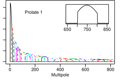
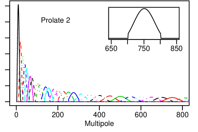
For spectral estimation, it is advisable to consider spectral window functions with relatively narrow spectral support, in order to reduce bias in the spectral estimation. The span of the summation in (4) can be fixed to some interval $[\ell_{\min}^{(j)},\ell_{\max}^{(j)}]$. For our illustrations, the interval bands have been chosen to cover the range of available multipoles with more bands around the expected positions of the peaks of the CMB. The bands are described in Table 1.

. Band $(j)$ 1 2 3 4 5 $\cdots$ 20 21 22 23 24 25 26 27 28 29 $\cdots$ 35 36 37 38 39 $\ell_{\min}^{(j)}$ 2 11 21 31 41 $\cdots$ 401 451 501 551 601 651 701 751 801 876 $\cdots$ 1326 1426 1501 1626 1751 $\ell_{\max}^{(j)}$ 20 30 40 50 60 500 550 600 650 700 750 800 875 950 1025 1475 1625 1750 1875 2000 $\texttt{nside}{}^{(j)}$ 16 16 32 32 32 $\cdots$ 256 512 512 512 512 512 512 512 512 1024 $\cdots$ 1024 1024 1024 1024 1024 $\theta_{0}^{(j)}$ 69 50 41 36 32 $\cdots$ 10.7 10.2 9.7 9.3 8.9 8.6 8.3 8.0 7.7 7.4 $\cdots$ 6.1 5.8 5.6 5.4 5.2

Table 1: Spectral bands used for the needlet decomposition in this analysis. Depending on $\ell_{\max}^{(j)}$, the needlet coefficient maps are computed using the HEALPix package, at different values of nside, given in the fourth line. The number $K^{(j)}$ of needlet coefficients in band $j$ is then $12(\texttt{nside}^{(j)})^{2}$. It is a kind of decimated implementation of the needlet transform. The last line gives the opening $\theta^{(j)}$ (in degrees) chosen in Eq. 26 to define the PSWF from the Prolate 2 family (see Section III.1.2 for details).

It is well known however that perfect spectral and spatial localization cannot be achieved simultaneously (call it the uncertainty principle). In order to reduce the effect of the mask, we have to check that the analysis kernels are well localized. This leads to the optimization of some localization criteria. If we retain the best $\mathbb{L}^{2}$ concentration in a polar cap $\Omega_{\theta^{(j)}}=\{\xi:\theta\leq\theta^{(j)}\}$, namely

$$(b^{(j)}_{\ell})_{\ell=\ell_{\min},\cdots,\ell_{\max}}\\ =\arg\max_{\textsf{b}}\frac{\int_{\Omega_{\theta^{(j)}}}\left|\sum_{\ell=\ell_{\min}^{(j)}}^{\ell_{\max}^{(j)}}{\textsf{b}}^{(j)}_{\ell}L_{\ell}(\xi)\right|^{2}\mathrm{d}\xi}{\int_{\mathbb{S}}\left|\sum_{\ell=\ell_{\min}^{(j)}}^{\ell_{\max}^{(j)}}\textsf{b}^{(j)}_{\ell}L_{\ell}(\xi)\right|^{2}\mathrm{d}\xi}$$ (26)

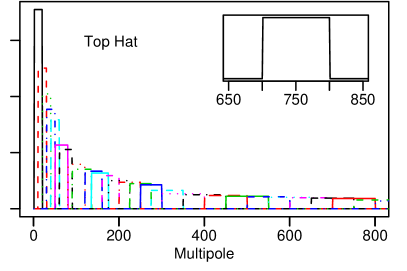
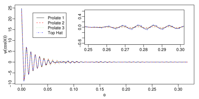
we obtain the analogous of prolate spheroidal wave function (PSWF) thoroughly studied in e.g. Slepian & Pollak (1960) for the PSWF in $\mathbb{R}$ and Simons et al., (2006); Guilloux et al., (2008) for PSWF on the sphere. In our simulations, we use PSWF needlets since they are well localized and easy to compute. Other criteria and needlets can be investigated and optimized, at least numerically; see Guilloux et al., (2008) for details. The choice of the optimal window function in a given band is a non trivial problem which involves the spectrum itself, the characteristics of the noise and the geometry of the mask. Even if we restrict to PSWF as we do here, it is not clear how to choose the optimal opening $\theta^{(j)}$ for each band $j$. We can use several rules of thumb based on approximate scaling relation between roughly $B$-adic bands and openings $\theta^{(j)}$ that preserve some Heisenberg product or Shannon number. Figure 1 represents three families of PSWF needlets that are numerically compared below. Their spatial concentration is illustrated by Figure 2.

Figure 1: Four families of window functions that are used for the NSE and compared numerically in Section III.1.2. There are three families of prolate spheroidal wave functions and one family of top-hat functions. All the families are defined on the same bands. Inset graphs show the window function in the 26th band. Each window function is normalized by the relation $(4\pi)^{-1}\sum(b_{\ell}^{(j)})^{2}(2\ell+1)=1$. Then, if the angular power spectrum is flat, $C_{\ell}\equiv C_{0}$, then $C^{(j)}\equiv C_{0}$ for all bands, according to (8).

Figure 2: Angular profile of the four needlets associated to the window functions at the 26th band ($701\leq\ell\leq 800$) from the four families of Figure 1. We have plotted the axisymmetric profile $\sum_{\ell}b_{\ell}L_{\ell}(\cos\theta)$ as a function of $\theta$. Needlets with “smoother” associated window profile (such as Prolate 3) need more room to get well localized, but are less bouncing than needlets with abrupt window function (such as top hat or Prolate 1)

II.3.2 The choice of the needlets coefficients (mask)

Practically we want to keep as much information (i.e. as many needlet coefficients) as possible, and to minimize the effect of the mask. Using all the needlet coefficients regardless of the mask would lead to a biased estimate of the spectrum. It is still true if we keep all the coefficients outside but still close to the mask, keeping in mind that the needlets are not perfectly localized. On the other hand, getting rid of unreliable coefficients reduces the bias, but increases the variance. This classical trade-off is taken by choosing the threshold level $t^{(j)}$ in the Definition (10) of the excluding zones. For multiple experiments, a different selection rule can be applied to each experiment, according to the geometry of the mask and the characteristics of the beam and the noise.

III Monte Carlo studies

Recall that NSE spectral estimators are designed based on three approximations:

• one can neglect the impact of the mask on the needlet coefficients which are centered far enough from its edges;

• one can neglect the variations of the beam and the CMB power spectrum over each band.

• the weights, which are optimal under the simplifying assumption of independent needlet coefficients, still provide good estimates for the truly weakly correlated needlet coefficients.

We carry out Monte Carlo studies to investigate, first the actual performance of the method on realistic data, and second the sensitivity of the method with respect to its parameters. Stochastic convergence results under appropriate conditions is established in a companion paper Faÿ and Guilloux, (2008).

III.1 Single map with a mask and inhomogeneous noise

In this section, we first consider model (2). According to Eqs (12) and (16), any beam can be taken into account easily in the procedure. Without loss of generality, we suppose here that there is no beam (or $B$ is the Dirac function). The case of different beams is addressed in Section III.2, see Table 2.

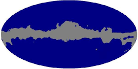
The key elements for this numerical experiment are illustrated by Fig. 3. We simulate CMB from the spectrum $C_{\ell}$ given by the $\Lambda$CDM model that best fits the W-MAP data. We use a Kp0 cut (Bennett et al.,, 2003) for the mask and we take a simple non homogeneous noise standard deviation map (the SNR per pixel is 1.5 in two small circular patches and 0.4 elsewhere).

(a) Mask

(b) Noise standard deviation

(c) One simulated input map

(d) Spectra

Figure 3: Simplified model of partially covered sky and inhomogeneous additive noise. This model is used to compare numerically the NSE estimator with PCL estimators and to assess the robustness or the sensitivity of the method with respect to its parameters. The mask is kp0. In CMB $\mu K$ units, the standard deviation of the uncorrelated pixel noise is 75 in the two small circular patches and 300 elsewhere.

Using a mean-square error criterion, we first study the dependence of NSE performance on its free parameters. Then we compare NSE with methods based on Spherical Harmonic coefficients, known as pseudo-$C_{\ell}$ estimation and followed in Hinshaw et al. (2006)). For the reader’s convenience, the PCL procedure is summarized in Appendix A.

III.1.1 Mean-square error

We shall measure the quality of any estimator $\widehat{C}^{(j)}$of $C^{(j)}$ by its mean-square error

$$\text{MSE}(\widehat{C}^{(j)})=\mathbb{E}\left(\widehat{C}^{(j)}-C^{(j)}\right)^{2}\ .$$

This expectation is estimated using 400 Monte Carlo replications. Roughly speaking, the MSE decomposes as an average estimation error and a sampling variance. The estimation error term is intrinsic to the method. Ideally, it should be used to compare the relative efficiency of concurrent approaches. The sampling variance term is the so-called cosmic variance. It is given by the characteristic of the spectrum and coming from the fact that we only have one CMB sky, and thus $2\ell+1$ $a_{\ell m}$’s to estimate one $C_{\ell}$. It is increased by the negative influence of the noise and the mask. This gives an error term intrinsic to the whole experiment. When the sky is partially observed (let $f_{\text{sky}}$ denote the fraction of available sky) and for high $\ell$’s (or $j$’s), the cosmic variance must be divided by a factor $f_{\text{sky}}$ leading to the following approximate Cramér-Rao lower bound at high frequencies

$$V_{\text{sample}}^{(j)}=f_{\text{sky}}^{-1}V_{\text{cosmic}}^{(j)}\ .$$ (27)

Including an homogeneous additive uncorrelated pixel noise with variance $\sigma^{2}$, the sample variance writes

$$2f_{\text{sky}}^{-1}\sum(b_{\ell}^{(j)})^{4}(2\ell+1)\left(C_{\ell}+\frac{4\pi}{N_{\text{pix}}}\sigma^{2}\right)^{2}$$

In a non-homogeneous context, no close expression for the sampling variance is available: Eq. (27) will serve as one reference. When comparing different window functions in the same band, it must be kept in mind that different estimators do not estimate the same $C^{(j)}$ so that the sampling variances are not the same. In this case, we use the following normalized MSE

$$\frac{\text{MSE}(\widehat{C}^{(j)})}{f_{\text{sky}}^{-1}V_{\text{cosmic}}^{(j)}}$$ (28)

III.1.2 Robustness with respect to parameter choice

This section looks into the robustness of NSE with respect to its free parameters.

First and as expected, the spectral estimation is very sensitive to the choice of the window functions. Even if we restrict to the PSWF, one has the freedom to choose a concentration radius $\theta^{(j)}$ for each band. We compare the mean-square error of the estimation for various choices of $\theta^{(j)}$ that lead to three of the window function families displayed in Figure 1. The second prolate family is obtained using the “rule of thumb” relation $\theta^{(j)}=2((\ell_{\min}^{(j)}+\ell_{\max}^{(j)})/2)^{-1/2}$. The values of those opening angles are in Table 1. The first and third sequences of opening angles are the same with a multiplicative factor of 0.5 and 2, respectively. For the sake of comparison we also consider the top-hat window functions. Figure 4 shows the normalized MSE for those four “families” of needlets as a function of the band index.

Figure 4: Comparison of the normalized MSE (28) of the needlet spectral estimators for the four families of spectral window functions displayed in Figure 1. The smoothness of the window function make the MSE smaller at high multipoles. At low multipoles, taking a too smooth function makes the needlet less localized and there is a loss of variance due to the smaller number ${\cal K}^{(j)}$ of needlet coefficients that are combined.

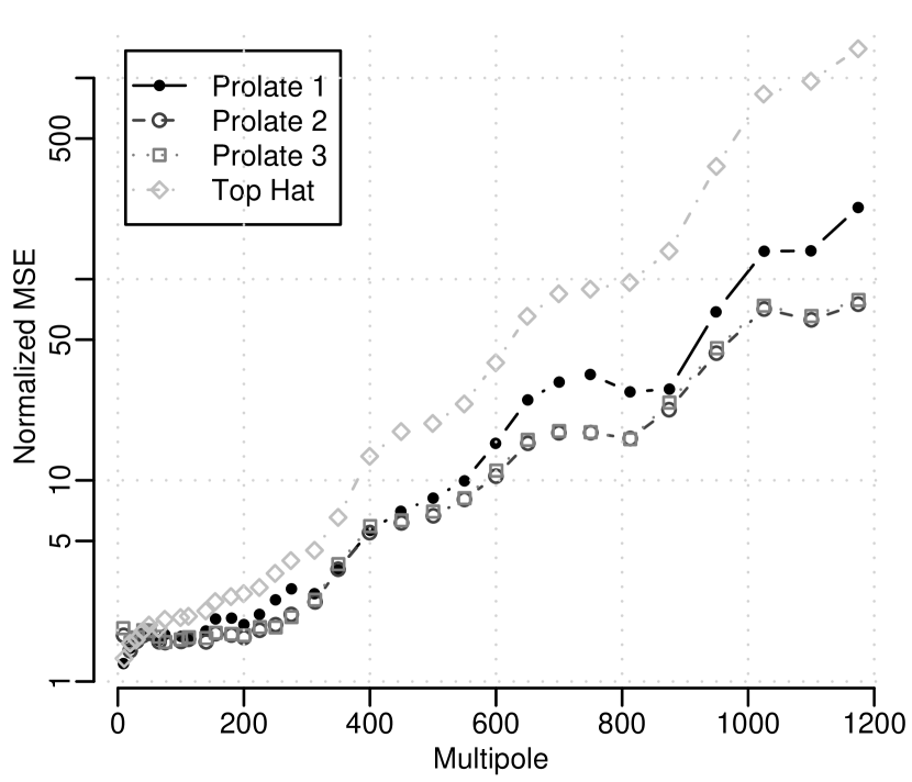
Notice the poor behavior of a non-optimized window function and the far better performance of the second prolate family in comparison with top-hat and Prolate 1 windows. Thus, in the following, we use this particular needlet family to study the sensitivity of the method with respect to the other parameters, and to compare NSE and PCL estimators.

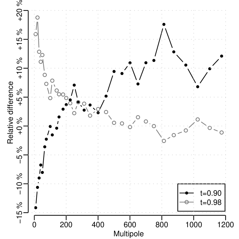
Next, for the second family of PSWF, we compare the influence of the threshold value $t^{(j)}\equiv t$ for $t=0.9,0.95$ or $0.98$. Figure 5 shows that this choice within reasonable values is not decisive in the results of the estimation procedure. For very low frequencies ($\ell\leq 100$), the conservative choice $t=0.98$ increases the variance since many needlets are contaminated by the mask and discarded. Qualitatively, in such variance dominated regimes, taking more coefficients (e.g. $t=0.9$) is adequate. However, we do not advocate the use of the NSE at low $\ell$’s where exact maximum likelihood estimation is doable. At higher $\ell$’s, there is roughly no difference between the $t=0.95$ and $t=0.98$ thresholds.

Figure 5: Relative difference between the normalized MSE (28) of the needlet spectral estimation using thresholds 0.9 and 0.98, and the same with threshold 0.95. It highlights the fact that the estimation is not very sensitive to the value of this parameter, except at low $\ell$’s, where we do not advocate the use of the NSE. The window function family is “Prolate 2” from Figure 1.

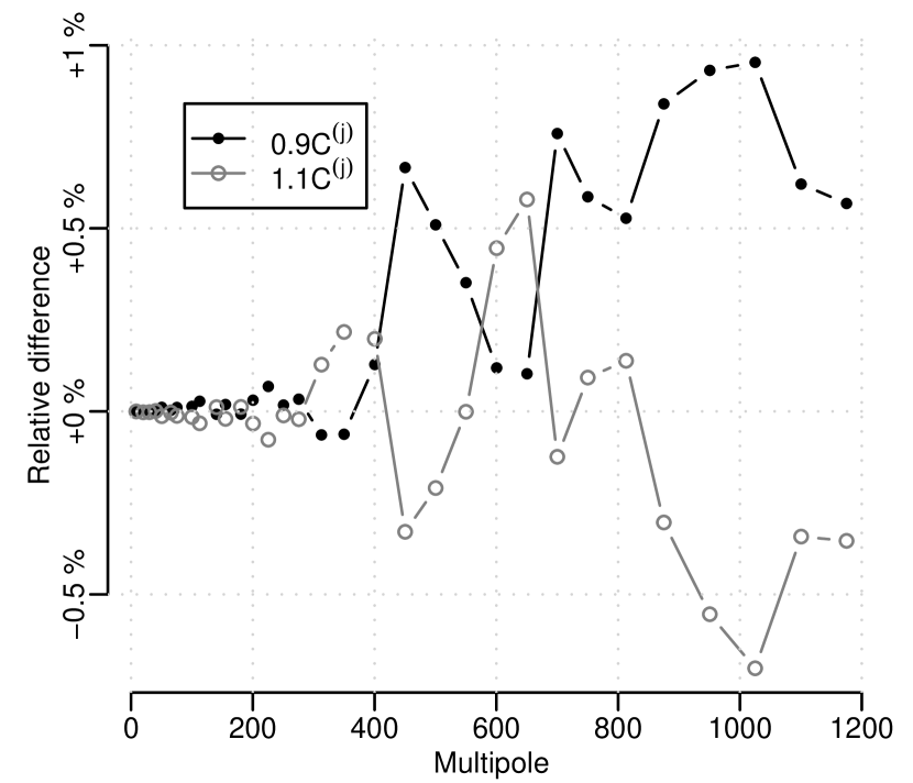
Finally, we check the robustness of the method against an imprecise initial spectrum. We take $0.9C^{(j)}$ and $1.1C^{(j)}$ as initial values $\bar{C}^{(j)}$ and compare the results with the best possible initial value which is $C^{(j)}$ itself. The relative difference between the results, displayed in Figure 6, does not exceed 1%.

Figure 6: Robustness of the NSE with respect to the initial value $\bar{C}^{(j)}$ given to the weights formula (18). We have performed the whole estimation with $\bar{C}^{(j)}=0.9C^{(j)}$ and $\bar{C}^{(j)}=1.1C^{(j)}$. This plot shows the relative difference between the normalized MSE under those initial values and the normalized MSE under the optimal initial value $\bar{C}^{(j)}=C^{(j)}$.

III.1.3 Pseudo-$C_{\ell}$ versus needlet spectral estimator

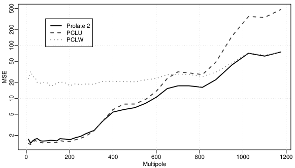
We compare the NSE estimator given by Eq. (16) with estimation based on the spherical Harmonic coefficients of the uniformly weighted map and of the $1/\sigma^{2}$-weighted map. The result is displayed in Fig. 7.

As expected, at low multipoles, where the SNR is higher, the uniform pseudo-$C_{\ell}$ estimator performs better than the weighted pseudo-$C_{\ell}$ estimator and, conversely, at high multipoles where the SNR is lower. Efstathiou, (2004) proved that the equal-weights pseudo-$C_{\ell}$ estimator is asymptotically Fisher-efficient when $\ell$ goes to infinity. The behaviour of the needlet estimator is excellent: its performance is comparable to the best of the two previous methods both at low and high multipoles. Thus, there is no need to choose arbitrary boundaries between frequencies for switching for one weighting to the other. The NSE estimator automatically implements a smooth transition between the two regimes and it does so quasi-optimally according to noise and mask characteristics. At low $\ell$’s one should optimize the window function (the characteristic angle of opening of the prolates) to broaden the range of optimality of the NSE.

Figure 7: Comparison of the relative MSE (28) of the two PCL estimators (PCLU for flat weights, PCLW for inverse variance weights) with the NSE, for Prolate family 2. For $300\leq\ell\leq 1200$, the NSE is uniformly better than the best of the two PCL methods. It should be noted that the NSE may be improved again by optimizing the window profiles and the thresholds $t^{(j)}$ (e.g. by taking a lower threshold for low bands to reduce the variance, see Figure 5).

Providing a $C_{\ell}$ estimate with error bars is often not sufficient. Estimate the covariance matrix of the whole vector of spectral estimates is necessary for full error propagation towards, say, estimates of cosmological parameters. Figure 8 shows the values of the correlation matrix between the spectral estimates. In the idealistic case of a full sky noiseless experiment, the theoretical correlation matrix is tridiagonal because window functions we have chosen only overlap with their left and right nearest neighbours. The mask induces a spectral leakage, which is however reduced for the smoothest window function. This leakage is however compensated for by the selection of coefficients in $\mathcal{K}^{(j)}_{t^{(j)}}$ (see Eq (10)).

Figure 8: Absolute value of the correlation matrix of vector $(\widehat{C}^{(1)},\ldots,\widehat{C}^{(32)})$, which entries are defined by Eq. (16). It has been estimated in the context of Fig. 3 using two different families of window functions and 400 Monte Carlo replicates. This shows the difference between a family of PSWF (left panel) and a family of top-hat windows (right panel).

III.2 Aggregation of multiple experiments

Historically in CMB anisotropy observations, no single instrument provides the best measurement everywhere on the sky, and for all possible scales. In the early 90’s, the largest scales have been observed first by COBE-DMR, complemented by many ground-based and balloon-borne measurements at higher $\ell$. Similarly, ten years later, WMAP full sky observations on large and intermediate scales have been complemented by small scale, local observations of the sky as those of Boomerang, Maxima, ACBAR or VSA.

The joint exploitation of such observations has been so far very basic. The best power spectrum is obtained by choosing, for each scale, the best measurement available, and discarding the others. One could, alternatively, average the measurements in some way, but the handling of errors is complicated in cases where a fraction of the sky is observed in common by more than one experiment.

Clearly, the data is best used if some method is devised that allows combining such complementary observations in an optimal way. In this section we present the results of a Monte Carlo study to illustrate the benefits of our method of aggregated spectral estimator.

We simulate observations following the model (3), with $E=6$ observed maps : 3 Kp0-masked maps with beams and noise-level maps according to W-MAP experiment in bands Q, V and W respectively ; 3 maps with uniform noise, observed in patches the size of which are equivalent to BOOMERanG-Shallow, BOOMERanG-Deep and ACBAR observations respectively, and noise levels representative of the sensitivities of those experiments. Table 2 gives the key features of these experiments.

Experiment	Beam	nside	Noise level	$f_{\text{sky}}$
W-MAP Q	31’	512	Given by the hit map	78.57 %
W-MAP V	21’
W-MAP W	13’
BOOM S	10’	1024	17.5 $\mu$K	2.80 %
BOOM D			5.2 $\mu$K	0.65 %
ACBAR	5’	2048	14.5 $\mu$K	1.62 %

Table 2: Main parameters of the experiments to be aggregated. The beams are given in minutes of arc, nside refers to HEALPix resolution of the simulated maps, noise level is either a map computed from a hitmap and an overall noise level, or a uniform noise level per pixel (in $\mu$K CMB). Numbers quoted here are indicative of the typical characteristics of observations as those of W-MAP, BOOMERanG and ACBAR, and are used for illustrative purposes only.

Further details can be found in Bennett et al., (2003) and Hinshaw et al., (2008) for W-MAP, Masi et al., (2006) for BOOMERanG, Runyan et al., (2003) and Reichardt et al., (2008) for ACBAR. However, we do not intend to produce fully-realistic simulations. Basically, no foregrounds are included in simulations (neither diffuse nor point sources) ; for ACBAR only the 3 sky fields of year 2002 are used ; and for W-MAP only one detector is used for each band.

Key elements for this numerical experiment are illustrated in Fig. 9-10-11, where we have displayed respectively one random outcome of each experiment according to those simplified models, the maps of local noise levels and power spectra of the CMB and of the experiment’s noise.

(a) “True” CMB

(b) WMAP-Q

(c) WMAP-V

(d) WMAP-W

(d) BOOMERanG-S

(e) BOOMERanG-D

(f) ACBAR

Figure 9: Simulated observations from model (3) for the 6 experiments described in Table 2, in a small patch around point (-40,-90). The approximate size of the patch is 38$\times$38 degrees.

(a) WMAP-Q

(b) WMAP-V

(c) WMAP-W

(d) BOOMERanG-S

(e) BOOMERanG-D

(f) ACBAR

Figure 10: Coverage and local pixel noise levels of the six simple experiments described in Table 2.

Figure 11: Spectra of the beamed CMB (with the BOOMERanG lines overplotted) and noise levels (horizontal lines) seen by the six experiments, as if they were full sky (the $f_{\text{sky}}$ effect is not taken into account).

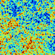
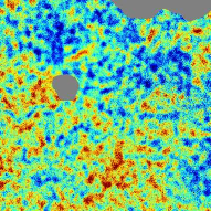
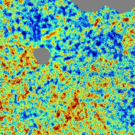
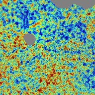
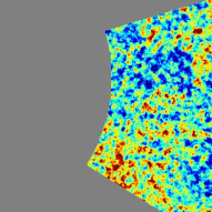
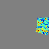
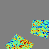
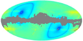
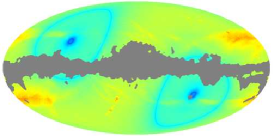
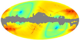
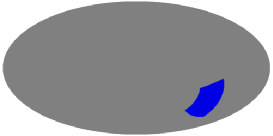
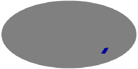
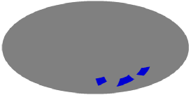
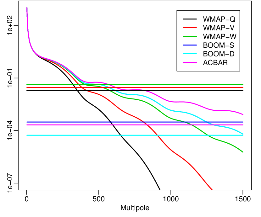
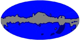
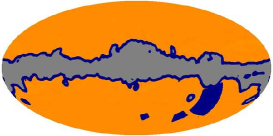
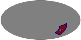
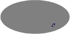
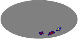
Fig. 13 displays the maps of the weights $\omega_{k,e}^{(26)}$ (the 26th band is the multipole range $700<\ell\leq 800$). According to Eq. (23), all those weights belong to [0,1] and for any fixed position, the sum of the weights over the six experiments is equal to one. Red regions indicates needlet coefficients which are far better observed in an experiment that in all others. Blue, light blue and orange region are increasing but moderately low weights, showing that outside the small patches of BOOMERanG and ACBAR, most information on band 26 is provided by the channel W of WMAP. On the patches, needlet coefficients from W-MAP are numerically neglected in the combination (21).

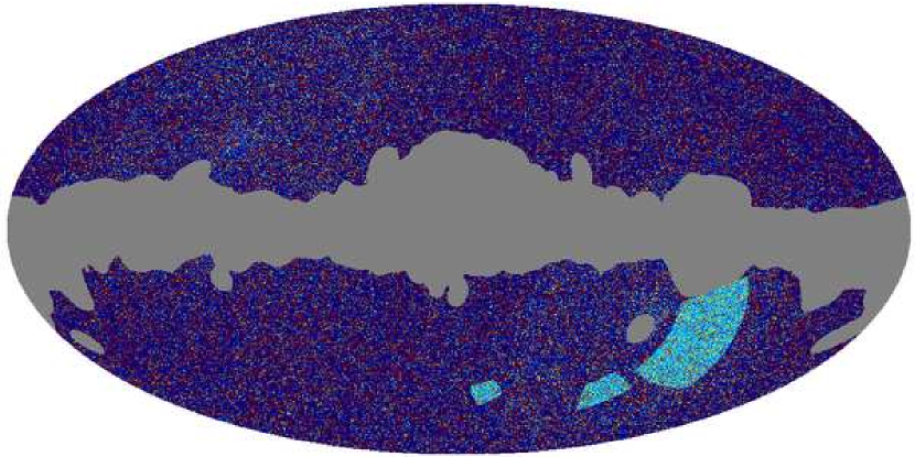
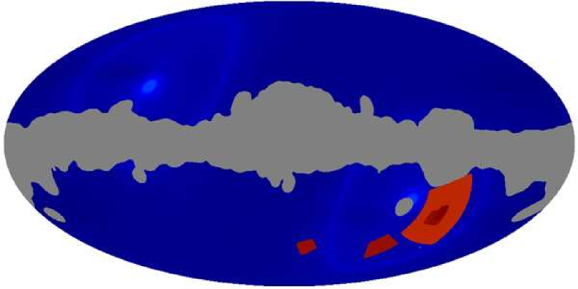
The debiased, squared, aggregated coefficients $\left(\tilde{\gamma}^{(26)}_{k}\right)^{2}-\left(\tilde{n}_{k}^{(26)}\right)^{2}$ are displayed on the left map from Fig. 14. All those coefficients are approximately unbiased estimators of $C^{(26)}$. The map of weights $\tilde{w}_{k}^{(26)}$ is displayed on the right of Figure 14. More weight is given to regions which are covered by lower noise experiments. The final estimate is obtained by averaging the pixelwise multiplication of these two maps.

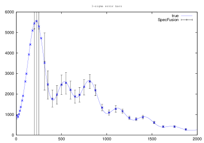
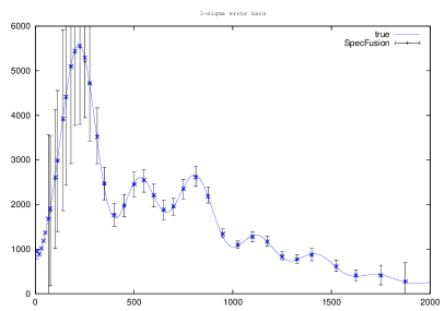
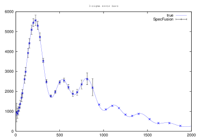
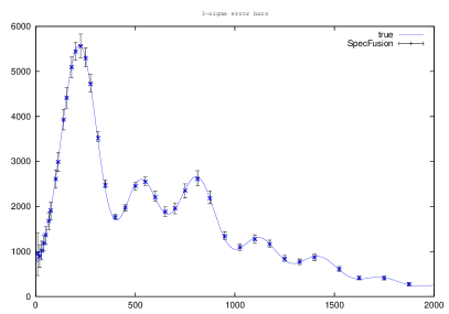
Figure 15 shows the benefit of the aggregation of different experiments, in comparison with separate estimations. In CMB literature, error bars from different experiments are usually plotted on a same graph with different colors. For easier reading, we plot the output of single experiment NSE in separate panels (a,b and c). Panel (d) shows the output of the aggregated NSE, which improve the best single experiment uniformly over the frequency range, thanks to the locally adaptive combination of informations from all expermiments.

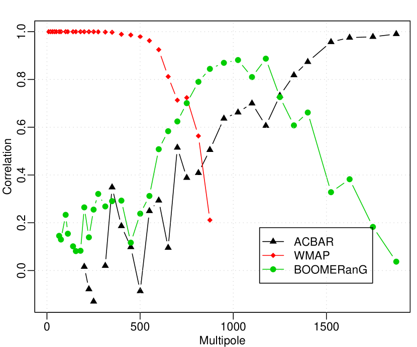
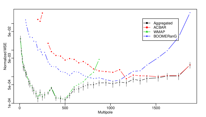
Figure 12 highlights the cross-correlation between single experiment estimators and the final aggregated estimator. It provides a complementary insight on the relative weight of each experiment in the spectral domain. The W-MAP-like measures are decisive for lower bands, whereas BOOMERanG and ACBAR ones give estimators very much correlated to the aggregated one at higher bands. The aggregated NSE is eventually almost identical to the estimator obtained from ACBAR alone.

Figure 12: Correlation between the aggregated estimator and single experiments estimators. This provides insight on the contribution of each experiment into the final aggregated single spectral estimate.

Figure 13: Method for aggregating experiments: Weights $\omega_{k,e}^{(26)}$ for combining the needlet coefficients from the 26th band $(700<\ell\leq 800)$ and the six experiments. From left to right and top to bottom: W-MAP-Q, W-MAP-V, W-MAP-W, BOOMERanG-S, BOOMERang-D and ACBAR.

Figure 14: Method for aggregating experiments: On the left: map of debiased squares of aggregated needlet coefficients, in the 26th band $(700<\ell\leq 800)$. On the right: map of the weights $w_{k}^{(j)}$ affected to those coefficients to estimate the power spectrum.

(a) ACBAR

(b) BOOMERanG

(c) WMAP

(d) All aggregated

Figure 15: Results for the aggregated NSE. Error bars are estimated by 100 Monte Carlo simulations. The ACBAR power spectrum is computed using the single map needlet estimator described in Section II.1, whereas the BOOMERanG and W-MAP spectra are obtained using the aggregation of needlets coefficients from the two (BOOM-S and BOOM-D) and three (W-MAP Q,V,W) maps respectively. The final spectrum (d) is obtained by aggregating all available needlet coefficients from the six maps.

Figure 16: Mean-square error of the three single expermiment NSE estimators and of the aggregated NSE estimator. The 2-sigmas error bars reflect the imprecision in the Monte Carlo estimation of the MSE of the aggregated NSE. Up to those uncertainties, the aggregated estimator is uniformly better than the best of all experiments. The improvement is decisive in “crossing” regions, where two expermiments perform comparably. The normalized MSE here is $\mathbb{E}(\hat{C}^{(j)}-C^{(j)})^{2}/(C^{(j)})^{2}$.

IV Discussion

Complexity

According to (5), the calculation of all the needlet coefficients takes one SHT and $j_{\max}$ inverse SHT, where $j_{\max}$ is the number of bands. The weights $w_{k}^{(j)}$, $\tilde{w}_{k}^{(j)}$ and $\omega_{k,e}^{(j)}$ are obtained using simple operations on maps, so that the overall cost of the (aggregated) NSE scales as $N_{\text{pix}}^{3/2}$ operations. This is comparable to the cost of the PCL methods.

Sensitivity to the noise knowledge

To be unbiased, the above described estimators require a perfect knowledge of the noise characteristics, as do Pseudo-$C_{\ell}$ estimators. In both cases, the uncertainty on the noise can be tackled using cross-spectrum, that removes the noise on the average provided that the noises from each experiment are independent. Indeed, for any pixel $k$ far enough from the masks of experiment $e$ and $e^{\prime}$, $e\neq e^{\prime}$, we have

$$\mathbb{E}[\gamma_{k,e}^{(j)}\gamma_{k,e^{\prime}}^{(j)}]=B_{e}^{(j)}B_{e^{\prime}}^{(j)}C^{(j)}.$$

Thus, an unbiased spectral estimator is given by

$$\widehat{C}^{(j)}_{\text{cross}}=\sum_{k\in\mathcal{K}^{(j)}}w_{k}^{(j)}\sum_{e\neq e^{\prime}}\left(B_{e}^{(j)}B_{e^{\prime}}^{(j)}\right)^{-1}\gamma_{k,e}^{(j)}\gamma_{k,e^{\prime}}^{(j)}$$ (29)

where the weights $w_{k}^{(j)}$ depend on a preliminary estimate of the spectrum and a possibly imprecise estimate of the local and aggregated noise levels that enter in the variance of $\gamma_{k,e}^{(j)}\gamma_{k,e^{\prime}}^{(j)}$. This has not been investigated numerically yet but we can conjecture the qualitative results of this approach: more robustness with respect to noise misspecification but greater error bars than the NSE with perfectly known noise levels. Moreover, adapting the procedure described in Polenta et al., (2005), one can test for noise misspecification, and for the correct removal of the noise by considering the difference between the NSE $\widehat{C}^{(j)}$ and cross-spectrum NSE $\widehat{C}^{(j)}_{\text{cross}}$.

V Conclusion

We have presented some potentialities of the needlets on the sphere for the angular power spectrum estimation. This tool is versatile and allows to treat consistently the estimation from a single map or from multiple maps. There remains many ways of improving or modify the method described in Section II.

In the future, it is likely that again complementary data sets will co-exist. This is the case, in particular, for polarisation, for which Planck will measure the large scale CMB power on large scales with moderate sensitivity, while ground-based experiments will measure very accurately polarisation on smaller scales. Extensions to polarisation of the approach presented hers will likely be important for the best exploitation of such observations.

Appendix A Pseudo-$C_{\ell}$ estimators

Let $T$ be a stationary process with power spectrum $(C_{\ell})_{\ell\geq 0}$, $\mathcal{W}$ an arbitrary weight function (or mask) and

$$\widetilde{C}_{\ell}(\mathcal{W})=\frac{1}{2\ell+1}\sum_{m=-\ell}^{\ell}|\langle Y_{\ell m},\mathcal{W}T\rangle|^{2}$$

the so-called pseudo-power spectrum of $T$ with mask $\mathcal{W}$. The ensemble-average of this quantity is related to the true power spectrum by the formula

$$\mathbb{E}(\widetilde{C}_{\ell})=\mathcal{M}_{\ell\ell^{\prime}}(\mathcal{W})C_{\ell^{\prime}}$$

where $\mathcal{M}_{\ell\ell^{\prime}}(\mathcal{W})$ is the doubly-infinite coupling matrix associated with $\mathcal{W}$, see Peebles, (1973); Hivon et al., (2002). If $U$ is a unit variance white pixel noise, denote by $V_{\ell}\equiv 4\pi\sigma^{2}/N_{\text{pix}}$ its “spectrum” (see Appendix B). Consider now the model $X=\mathcal{W}_{1}T+\mathcal{W}_{2}U$. Then, if $\mathcal{M}_{\ell\ell^{\prime}}(\mathcal{W}_{1})$ is full-rank,

$$(\mathcal{M}_{\ell\ell^{\prime}}(\mathcal{W}_{1}))^{-1}\left\{\widetilde{C}_{\ell}(\mathcal{W}_{1})-\mathcal{M}(\mathcal{W}_{2})_{\ell\ell^{\prime}}V_{\ell^{\prime}}\right\}$$

is an unbiased estimator of $C_{\ell^{\prime}}$. It is obtained by deconvolving and debiasing the empirical spectrum. The observation model (2) with no beam coincides with the preceding framework with $\mathcal{W}_{1}=W$ and $\mathcal{W}_{2}=\sigma W$. This leads to the uniform-weights pseudo-$C_{\ell}$ estimator (PCLU). One can also divide all the observations by $\sigma^{2}$, yielding to a similar scheme with $\mathcal{W}_{1}=\sigma^{-2}W$ and $\mathcal{W}_{2}=\sigma^{-1}W$. This is the variance-weighted pseudo-$C_{\ell}$ estimator (PCLW). Both are used by the W-MAP collaboration (Hinshaw et al.,, 2007). The uniform weights lead to better estimates in the high SNR regime (low $\ell$’s) whereas the flat weights perform better at low SNR (high $\ell$’s). Efstathiou, (2004) showed that the Pseudo-$C_{\ell}$ estimator is statistically equivalent to the maximum likelihood estimator asymptotically as $\ell$ goes to infinity. He also proposed an implementation of a smooth transition between those two regimes.

Appendix B What “noise spectrum” means

Let $\nu$ denote the noise. It is defined on pixels and supposed centered, Gaussian, independent from pixel to pixel, and of variance $\sigma^{2}(\xi)$, i.e.

$$\nu_{k}=\sigma(\xi_{k})U_{k},\quad k=1,\dots N_{\text{pix}},$$

with $U_{1},\dots,U_{N_{\text{pix}}}\stackrel{{\scriptstyle\textrm{\tiny{i.i.d}}}}{{\sim}}\mathcal{N}(0,1)$. Define $\nu_{\ell m}:=\sum_{k}\lambda_{k}\nu_{k}Y_{\ell m}(\xi_{k})$, and call them (abusively) the “discretized” multipole moments of the noise, which do not have any continuous counterpart because $\nu$ is not defined on the whole sphere. Define the corresponding discretized empirical spectrum $\overline{N_{\ell}}:=\frac{1}{2\ell+1}\sum_{m}\nu_{\ell m}^{2}$, then

$$\mathbb{E}(\nu_{\ell m}\nu_{\ell^{\prime}m^{\prime}})=\sum_{k}\lambda^{2}_{k}\sigma^{2}(\xi_{k})Y_{\ell m}(\xi_{k})Y_{\ell^{\prime}m^{\prime}}(\xi_{k})$$

$$\overline{N_{\ell}}=\frac{1}{2\ell+1}\sum_{k,k^{\prime}}\lambda_{k}\lambda_{k^{\prime}}\sigma(\xi_{k})\sigma(\xi_{k^{\prime}})U_{k}U_{k^{\prime}}L_{\ell}(\langle\xi_{k},\xi_{k^{\prime}}\rangle)$$

$$\text{and}\quad\mathbb{E}(\overline{N_{\ell}})=\frac{1}{4\pi}\sum_{k}\lambda^{2}_{k}\sigma^{2}(\xi_{k})=:N_{\ell}$$

This sequence $N_{\ell}$ can be thought of as the pixel-noise spectrum. Note that if $\lambda_{k}=\frac{4\pi}{N_{pix}}$, $k=1,\dots,N_{\text{pix}}$, then $N_{\ell}=\frac{1}{N_{pix}}\int\sigma^{2}(\xi)\mathrm{d}\xi$. If the noise is moreover homogeneous, $\sigma(\xi)\equiv\sigma$, then $\mathbb{E}(\nu_{\ell m}\nu_{\ell^{\prime}m^{\prime}})=\frac{4\pi\sigma^{2}}{N_{pix}}\delta_{\ell,\ell^{\prime}}\delta_{m,m^{\prime}}$.

Appendix C Variance estimation by aggregation of experiments with independent heteroscedastic noise

Consider the model

$$Y_{k,e}=X_{k}+n_{k,e}Z_{k,e}$$

where $\mathbf{X}:=[X_{k}]_{k\in[1,N_{\text{pix}}]}$ and $\mathbf{Z}:=[Z_{k,e}]_{(k,e)\in[1,N_{\text{pix}}]\times[1,E]}$ are independent, $X_{k}\stackrel{{\scriptstyle\textrm{\tiny{i.i.d}}}}{{\sim}}\mathcal{N}(0,C)$, $Z_{k,e}\stackrel{{\scriptstyle\textrm{\tiny{i.i.d}}}}{{\sim}}\mathcal{N}(0,1)$ and the noise standard deviations $n_{k,e}$ are known. This corresponds to the observation of the same signal $\mathbf{X}$ by $E$ independent experiments, the observations being tainted by independent but heteroscedastic errors. Let $\mathbf{Y}_{k}:=[Y_{k,e}]_{(e\in[1,E]}$ be the vector of observations at point (or index in a general framework) $k$, and let $\mathbf{Y}:=([\mathbf{Y}_{k}^{T}]_{k\in[1,N_{\text{pix}}]})^{T}$ be the full vector of observations. The covariance matrix of $\mathbf{Y}_{k}$ is $\mathbf{R}_{k}:={\mathbf{1}}{\mathbf{1}}^{T}C+\mathbf{N}_{k}$ where $\mathbf{N}_{k}:=\text{diag}(n_{k,e}^{2})_{e\in[1,E]}$ and ${\mathbf{1}}$ is the $E\times 1$ vector of ones. By independence of the $\mathbf{Y}_{k}$’s, the negative log-likelihood of $C$ given $\mathbf{Y}$ thus writes

$$\mathcal{L}(C):=-2\log\left(P(\mathbf{Y}|C)\right) = -2\sum\nolimits_{k}\log\left(P(\mathbf{Y}_{k}|C)\right)$$

$$= \sum\nolimits_{k}{\mathbf{Y}_{k}}^{T}\mathbf{R}_{k}^{-1}\mathbf{Y}_{k}+\log\det\mathbf{R}_{k}.$$

Denote

$$\tilde{n}_{k}:=\left({\mathbf{1}}^{T}\mathbf{N}_{k}^{-1}{\mathbf{1}}\right)^{-1/2}=\left(\sum\nolimits_{e}\left({n_{k,e}}\right)^{-2}\right)^{-1/2}.$$ (30)

It is immediate to check the following identity which will be used below:

$$\mathbf{R}_{k}^{-1}{\mathbf{1}}=\frac{\mathbf{N}_{k}^{-1}{\mathbf{1}}}{1+C\tilde{n}_{k}^{2}}.$$

Define $\widehat{\mathbf{R}}_{k}:=\mathbf{Y}_{k}{\mathbf{Y}_{k}}^{T}$. The derivative of the negative log-likelihood writes

$$\mathcal{L}^{\prime}(C)= \sum\nolimits_{k}-{\mathbf{Y}_{k}}^{T}\mathbf{R}_{k}^{-1}\frac{\partial\mathbf{R}_{k}}{\partial C}\mathbf{R}_{k}^{-1}\mathbf{Y}_{k}+\text{tr }\left(\mathbf{R}_{k}^{-1}\frac{\partial\mathbf{R}_{k}}{\partial C}\right)$$

$$= \sum\nolimits_{k}\text{tr }\left(-{\mathbf{Y}_{k}}^{T}\mathbf{R}_{k}^{-1}{\mathbf{1}}{\mathbf{1}}^{T}\mathbf{R}_{k}^{-1}\mathbf{Y}_{k}\right)+\text{tr }\left(\mathbf{R}_{k}^{-1}{\mathbf{1}}{\mathbf{1}}^{T}\right)$$

$$= \sum\nolimits_{k}{\mathbf{1}}^{T}\mathbf{R}_{k}^{-1}\left(\mathbf{R}_{k}-\widehat{\mathbf{R}}_{k}\right)\mathbf{R}_{k}^{-1}{\mathbf{1}}$$

$$= \sum\nolimits_{k}\frac{{\mathbf{1}}^{T}\mathbf{N}_{k}^{-1}\left(\mathbf{R}_{k}-\widehat{\mathbf{R}}_{k}\right)\mathbf{N}_{k}^{-1}{\mathbf{1}}}{\left(1+C\tilde{n}_{k}^{2}\right)^{2}}$$

$$= C\sum\nolimits_{k}\frac{\left({\mathbf{1}}^{T}\mathbf{N}_{k}^{-1}{\mathbf{1}}\right)^{2}}{\left(1+C\tilde{n}_{k}^{2}\right)^{2}}-\sum\nolimits_{k}\frac{\left({\mathbf{1}}^{T}\mathbf{N}_{k}^{-1}\mathbf{Y}_{k}\right)^{2}-{\mathbf{1}}^{T}\mathbf{N}_{k}^{-1}{\mathbf{1}}}{\left(1+C\tilde{n}_{k}^{2}\right)^{2}}$$

$$= C\sum\nolimits_{k}\left(C+\tilde{n}_{k}^{2}\right)^{-2}-\sum\nolimits_{k}\frac{\left(\tilde{n}_{k}^{2}{\mathbf{1}}^{T}\mathbf{N}_{k}^{-1}\mathbf{Y}_{k}\right)^{2}-\tilde{n}_{k}^{2}}{\left(C+\tilde{n}_{k}^{2}\right)^{2}}.$$

It follows that the likelihood is maximized for

$$C=\widehat{C}(w):=\sum\nolimits_{k}w_{k}(C,\mathbf{N})\left[\left(\tilde{n}_{k}^{2}{\mathbf{1}}^{T}\mathbf{N}_{k}^{-1}\mathbf{Y}_{k}\right)^{2}-\tilde{n}_{k}^{2}\right]$$

with

$$w_{k}(C,\mathbf{N}):=\left(C+\tilde{n}_{k}^{2}\right)^{-2}\left[\sum\nolimits_{i}\left(C+\tilde{n}_{i}^{2}\right)^{-2}\right]^{-1}.$$ (31)

As the optimal weights depend on $C$, this only defines implicitly the ML estimator. For some approximate spectrum $C^{0}$, the proposed explicit NSE is given by $\widehat{C}(\widehat{w}_{k})$ with $\widehat{w}_{k}=w_{k}(C^{0},\mathbf{N})$.

Particular case of a single experiment

In the particular case of a single experiment ($E=1$) with heteroscedastic noise, following the model

$$Y_{k}=X_{k}+n_{k}Z_{k}\;,$$

the likelihood is maximized for

$$C=\widehat{C}(w):=\sum\nolimits_{k}w_{k}(C,\mathbf{N})\left(Y_{k}^{2}-n_{k}^{2}\right)$$ (32)

with $w_{k}(C,\mathbf{N})$ defined by Eq. (31), and again, assuming that $w_{k}$ is poorly sensitive to $C$, the NSE is $\widehat{C}\left(\widehat{w}_{k}(C^{0})\right)$ for some approximate spectrum $C^{0}$.

References

- Baldi et al., (2007) Baldi, P., Kerkyacharian, G., Marinucci, D., and Picard, D. (2007). Subsampling Needlet Coefficients on the Sphere. ArXiv e-prints, 706.
- (2) Baldi, P., Kerkyacharian, G., Marinucci, D., and Picard, D. (2008a). Asymptotics for spherical needlets. Ann. Statist. To appear. arxiv.org: math.ST/0606154.
- (3) Baldi, P., Kerkyacharian, G., Marinucci, D., and Picard, D. (2008b). High frequency asymptotics for wavelet-based tests for Gaussianity and isotropy on the torus. J. Multivariate Analysis, 99:606–636.
- Bennett et al., (2003) Bennett, C. L., Halpern, M., Hinshaw, G., Jarosik, N., Kogut, A., Limon, M., Meyer, S. S., Page, L., Spergel, D. N., Tucker, G. S., Wollack, E., Wright, E. L., Barnes, C., Greason, M. R., Hill, R. S., Komatsu, E., Nolta, M. R., Odegard, N., Peiris, H. V., Verde, L., and Weiland, J. L. (2003). First-Year Wilkinson Microwave Anisotropy Probe (WMAP) Observations: Preliminary Maps and Basic Results. ApJS, 148:1–27.
- Bond et al., (1998) Bond, J. R., Jaffe, A. H., and Knox, L. (1998). Estimating the power spectrum of the cosmic microwave background. Phys. Rev. D, 57(4):2117–2137.
- Dahlen and Simons, (2008) Dahlen, F. A. and Simons, F. J. (2008). Spectral estimation on a sphere in geophysics and cosmology. Geophys. J. Int., page in press.
- Daubechies, (1992) Daubechies, I. (1992). Ten lectures on wavelets, volume 61 of CBMS-NSF Regional Conference Series in Applied Mathematics. Society for Industrial and Applied Mathematics (SIAM), Philadelphia, PA.
- Delabrouille et al., (2008) Delabrouille, J., Cardoso, J.-F., Le Jeune, M., Betoule, M., Faÿ, G., and Guilloux, F. (2008). A full sky, low foreground, high resolution CMB map from WMAP. Submitted to A&A, arxiv:astro-ph/0807.0773.
- Efstathiou, (2004) Efstathiou, G. (2004). Myths and truths concerning estimation of power spectra: the case for a hybrid estimator. Monthly Notices of the Royal Astronomical Society, 349(2):603–626.
- Eriksen et al., (2004) Eriksen, H. K. et al. (2004). Power spectrum estimation from high-resolution maps by Gibbs sampling. Astrophys. J. Suppl., 155:227–241.
- Faÿ and Guilloux, (2008) Faÿ, G. and Guilloux, F. (2008). Consistency of a needlet spectral estimator on the sphere.
- Górski et al., (2005) Górski, K., Hivon, E., Banday, A., Wandelt, B., Hansen, F., Reinecke, M., and Bartelmann, M. (2005). HEALPix: A Framework for High-Resolution Discretization and Fast Analysis of Data Distributed on the Sphere. Astrophys. J., 622:759–771. Package available at http://healpix.jpl.nasa.gov.
- Guilloux et al., (2008) Guilloux, F., Faÿ, G., and Cardoso, J.-F. (2008). Practical wavelet design on the sphere. Appl. Comput. Harmon. Anal. (In press) http://dx.doi.org/10.1016/j.acha.2008.03.003.
- Hinshaw et al., (2007) Hinshaw, G., Nolta, M., Bennett, C., Bean, R., Dore, O., Greason, M., Halpern, M., Hill, R., Jarosik, N., Kogut, A., Komatsu, E., Limon, M., Odegard, N., Meyer, S., Page, L., Peiris, H., Spergel, D., Tucker, G., Verde, L., Weiland, J., Wollack, E., and Wright, E. (2007). Three-Year Wilkinson Microwave Anisotropy Probe (WMAP) Observations: Temperature Analysis. Astrophys. J. Supp. Series, 170:288–334.
- Hinshaw et al., (2003) Hinshaw, G., Spergel, D. N., Verde, L., Hill, R. S., Meyer, S. S., Barnes, C., Bennett, C. L., Halpern, M., Jarosik, N., Kogut, A., Komatsu, E., Limon, M., Page, L., Tucker, G. S., Weiland, J. L., Wollack, E., and Wright, E. L. (2003). First-Year Wilkinson Microwave Anisotropy Probe (WMAP) Observations: The Angular Power Spectrum. Astrophys. J., 148:135–159.
- Hinshaw et al., (2008) Hinshaw, G., Weiland, J. L., Hill, R. S., Odegard, N., Larson, D., Bennett, C. L., Dunkley, J., Gold, B., Greason, M. R., Jarosik, N., Komatsu, E., Nolta, M. R., Page, L., Spergel, D. N., Wollack, E., Halpern, M., Kogut, A., Limon, M., Meyer, S. S., Tucker, G. S., and Wright, E. L. (2008). Five-Year Wilkinson Microwave Anisotropy Probe (WMAP) Observations: Data Processing, Sky Maps, and Basic Results. arXiv:0712.1148.
- Hivon et al., (2002) Hivon, E., Górski, K. M., Netterfield, C. B., Crill, B. P., Prunet, S., and Hansen, F. (2002). MASTER of the Cosmic Microwave Background anisotropy power spectrum: A fast method for statistical analysis of large and complex Cosmic Microwave Background data sets. The Astrophysical Journal, 567:2–17.
- Leach et al., (2008) Leach, S. M., Cardoso, J. ., Baccigalupi, C., Barreiro, R. B., Betoule, M., Bobin, J., Bonaldi, A., de Zotti, G., Delabrouille, J., Dickinson, C., Eriksen, H. K., González-Nuevo, J., Hansen, F. K., Herranz, D., LeJeune, M., López-Caniego, M., Martinez-González, E., Massardi, M., Melin, J. ., Miville-Deschênes, M. ., Patanchon, G., Prunet, S., Ricciardi, S., Salerno, E., Sanz, J. L., Starck, J. ., Stivoli, F., Stolyarov, V., Stompor, R., and Vielva, P. (2008). Component separation methods for the Planck mission. ArXiv e-prints, 805.
- Marinucci et al., (2008) Marinucci, D., Pietrobon, D., Balbi, A., Baldi, P., Cabella, P., Kerkyacharian, G., Natoli, P., Picard, D., and Vittorio, N. (2008). Spherical Needlets for CMB Data Analysis. M.N.R.A.S., 383(2):539–545.
- Masi et al., (2006) Masi, S., Ade, P. A. R., Bock, J. J., Bond, J. R., Borrill, J., Boscaleri, A., Cabella, P., Contaldi, C. R., Crill, B. P., de Bernardis, P., de Gasperis, G., de Oliveira-Costa, A., de Troia, G., di Stefano, G., Ehlers, P., Hivon, E., Hristov, V., Iacoangeli, A., Jaffe, A. H., Jones, W. C., Kisner, T. S., Lange, A. E., MacTavish, C. J., Marini Bettolo, C., Mason, P., Mauskopf, P. D., Montroy, T. E., Nati, F., Nati, L., Natoli, P., Netterfield, C. B., Pascale, E., Piacentini, F., Pogosyan, D., Polenta, G., Prunet, S., Ricciardi, S., Romeo, G., Ruhl, J. E., Santini, P., Tegmark, M., Torbet, E., Veneziani, M., and Vittorio, N. (2006). Instrument, method, brightness, and polarization maps from the 2003 flight of BOOMERanG. A&A, 458:687–716.
- Mayeli, (2008) Mayeli, A. (2008). Asymptotic uncorrelation for mexican needlets. (Preprint) arxiv : 0806.3009.
- Narcowich et al., (2006) Narcowich, F., Petrushev, P., and Ward, J. (2006). Localized tight frames on spheres. SIAM J. Math. Anal., 38(2):574–594.
- Peebles, (1973) Peebles, P. J. E. (1973). Statistical analysis of catalogs of extragalactic objects. I. Theory. Astrophys. J., 185:413–440.
- Pietrobon et al., (2006) Pietrobon, D., Balbi, A., and Marinucci, D. (2006). Integrated Sachs-Wolfe effect from the cross correlation of WMAP3 year and the NRAO VLA sky survey data: New results and constraints on dark energy. Phys. Rev. D, 74.
- Polenta et al., (2005) Polenta, G., Marinucci, D., Balbi, A., de Bernardis, P., Hivon, E., Masi, S., Natoli, P., and Vittorio, N. (2005). Unbiased estimation of an angular power spectrum. Journal of Cosmology and Astroparticle Physics, 2005(11):001.
- Reichardt et al., (2008) Reichardt, C. L., Ade, P. A. R., Bock, J. J., Bond, J. R., Brevik, J. A., Contaldi, C. R., Daub, M. D., Dempsey, J. T., Goldstein, J. H., Holzapfel, W. L., Kuo, C. L., Lange, A. E., Lueker, M., Newcomb, M., Peterson, J. B., Ruhl, J., Runyan, M. C., and Staniszewski, Z. (2008). High resolution CMB power spectrum from the complete ACBAR data set. ArXiv e-prints, 801.
- Runyan et al., (2003) Runyan, M. C., Ade, P. A. R., Bhatia, R. S., Bock, J. J., Daub, M. D., Goldstein, J. H., Haynes, C. V., Holzapfel, W. L., Kuo, C. L., Lange, A. E., Leong, J., Lueker, M., Newcomb, M., Peterson, J. B., Reichardt, C., Ruhl, J., Sirbi, G., Torbet, E., Tucker, C., Turner, A. D., and Woolsey, D. (2003). ACBAR: The Arcminute Cosmology Bolometer Array Receiver. ApJS, 149:265–287.
- Simons et al., (2006) Simons, F. J., Dahlen, F. A., and Wieczorek, M. A. (2006). Spatiospectral concentration on a sphere. SIAM Rev., 48(504).
- Slepian and Pollak, (1960) Slepian, D. and Pollak, H. (1960). Prolate spheroidal wave functions, Fourier analysis and uncertainty — I. Bell Syst. Tech. J., 40(1):43–63.
- Tegmark, (1997) Tegmark, M. (1997). How to measure cmb power spectra without losing information. Phys. Rev. D, 55(10):5895–5907.
- Wandelt et al., (2004) Wandelt, B. D., Larson, D. L., and Lakshminarayanan, A. (2004). Global, exact cosmic microwave background data analysis using gibbs sampling. Phys. Rev. D, 70(8):083511.
- Wieczorek and Simons, (2007) Wieczorek, M. A. and Simons, F. J. (2007). Minimum-variance spectral analysis on the sphere. J. Fourier Anal. Appl., 13(6):665–692, 10.1007/s00041–006–6904–1.