Transverse-momentum distributions in a diquark spectator model

Alessandro Bacchetta alessandro.bacchetta@jlab.org Theory Center, Jefferson Lab, 12000 Jefferson Av., Newport News, VA 23606, USA    Francesco Conti francesco.conti@pv.infn.it Dipartimento di Fisica Nucleare e Teorica, Università di Pavia, I-27100 Pavia, Italy Istituto Nazionale di Fisica Nucleare, Sezione di Pavia, I-27100 Pavia, Italy    Marco Radici marco.radici@pv.infn.it Istituto Nazionale di Fisica Nucleare, Sezione di Pavia, I-27100 Pavia, Italy
Abstract

All the leading-twist parton distribution functions are calculated in a spectator model of the nucleon, using scalar and axial-vector diquarks. Single gluon rescattering is used to generate T-odd distribution functions. Different choices for the diquark polarization states are considered, as well as a few options for the form factor at the nucleon-quark-diquark vertex. The results are listed in analytic form and interpreted in terms of light-cone wave functions. The model parameters are fixed by reproducing the phenomenological parametrization of unpolarized and helicity parton distributions at the lowest available scale. Predictions for the other parton densities are given and, whenever possible, compared with available phenomenological parametrizations.

pacs:
12.39.-x, 13.60.-r, 13.88.+e
preprint: JLAB-THY-08-841

I Introduction

Partonic transverse-momentum distributions (TMDs) — also called unintegrated PDFs — describe the probability to find in a hadron a parton with longitudinal momentum fraction x𝑥x and transverse momentum pTsubscript𝑝𝑇{p}_{\scriptscriptstyle T} with respect to the direction of the parent hadron momentum Collins:1982uw . They give a three-dimensional view of the parton distribution in momentum space, complementary to what can be obtained through generalized parton distributions Burkardt:2000za ; Diehl:2002he ; Ji:2003ak ; Belitsky:2003nz ; Boffi:2007yc .

In the last years a lot of theoretical and experimental activity related to TMDs has taken place. Crucial steps were made in the understanding of factorization theorems involving TMDs (kTsubscript𝑘𝑇k_{\scriptscriptstyle T} factorization)Ji:2004wu ; Ji:2004xq . Some of the properties of TMDs have been investigated from the theoretical standpoint. For instance, positivity bounds were presented in Ref. Bacchetta:1999kz . Relations among these functions in the large-Ncsubscript𝑁𝑐N_{c} limit of QCD were put forward in Ref. Pobylitsa:2003ty . Their behavior at large x𝑥x was studied in Ref. Brodsky:2006hj , and at high transverse momentum in Ref. Bacchetta:2008xw . Last but not least, it was also demonstrated Brodsky:2002cx that TMDs that are odd under naïve time-reversal transformations (for brevity, T-odd) can be nonzero and must be included in the complete list of leading-twist TMDs (see, e.g., Ref. Boer:1997nt ; Bacchetta:2006tn ). Their universality properties are different from the standard PDFs Collins:2002kn .

In the meanwhile, several azimuthal asymmetries were measured in semi-inclusive deep inelastic scattering (SIDIS) and elsewhere (see Ref. D'Alesio:2007jt and references therein), and more experimental measurements are planned. However, not much phenomenological information concerning TMDs is available as yet (see, e.g., Ref. D'Alesio:2004up and references therein). The analysis of azimuthal spin asymmetries both in hadron-hadron collisions and in SIDIS led to the extraction of the Sivers function Sivers:1990cc , denoted as f1Tsuperscriptsubscript𝑓1𝑇perpendicular-tof_{1T}^{\perp}, a T-odd TMD that describes how the parton distribution is distorted by the transverse polarization of the parent hadron (see Ref. Anselmino:2005an for a comparison of various parametrizations). A recent attempt to extract the T-odd Boer-Mulders function, h1superscriptsubscript1perpendicular-toh_{1}^{\perp} Boer:1998nt , a T-odd TMD describing the distribution of transversely polarized partons in an unpolarized hadron, was presented in Ref. Zhang:2008nu . All of the above studies assume a flavor-independent Gaussian distribution of the transverse momentum, although there is no compelling reason for this choice.

In this context, building a relatively simple model to compute TMDs and to allow for numerical estimates is of great importance. From the theoretical side, this can help understanding some of the essential features of TMDs, for instance their relation to the orbital angular momentum of partons (see, e.g., Refs. Brodsky:2002cx ; Brodsky:2002rv ; Burkardt:2003je ; Goeke:2006ef ; Lu:2006kt ; Meissner:2007rx ; Qiu:2007ey ; Burkardt:2007xm ). From the experimental side, a model could be useful to estimate the size of observables in different processes and kinematical regimes Gamberg:2003ey ; Gamberg:2003eg ; Lu:2004au ; Gamberg:2005ip ; Barone:2006ws ; Lu:2007ev ; Gamberg:2007wm and to set up Monte Carlo simulations Bianconi:2004wu ; Bianconi:2005bd ; Bianconi:2005yj ; Bianconi:2006hc ; Radici:2007vc .

Although many model calculations of integrated PDFs are available, there are not so many for TMDs. In Ref. Jakob:1997wg all the leading-twist T-even functions were calculated in a spectator model with scalar and axial-vector diquarks. Recently, an analogous calculation has been performed in a light-cone quark model Pasquini:2008ax . T-odd functions were calculated in the spectator model with scalar diquarks Brodsky:2002cx ; Boer:2002ju ; Goldstein:2002vv ; Gamberg:2003ey , with scalar and vector diquarks Bacchetta:2003rz ; Gamberg:2007wm , in the MIT bag model Yuan:2003wk ; Cherednikov:2006zn , in a constituent quark model Courtoy:2008vi and in the spectator model for the pion Lu:2004hu . A complete calculation of all the leading-twist TMDs in a spectator model with scalar diquarks was presented in Ref. Meissner:2007rx .

In this work, we choose a more phenomenological approach. We consider also axial-vector diquarks (in the following often called simply vector diquarks), necessary for a realistic flavor analysis, and we further distinguish between isoscalar (ud𝑢𝑑ud-like) and isovector (uu𝑢𝑢uu-like) spectators. We generate the relative phase necessary to produce T-odd structures by approximating the gauge link operator with a one gluon-exchange interaction. We consider several choices of form factors at the nucleon-quark-diquark vertex and several choices for the polarization states of the diquark. All results are presented in analytic form and interpreted also in terms of overlaps of light-cone wave functions, leading to a detailed analysis of the quantum numbers of the quark-diquark system. The free parameters of the model are fixed by reproducing the phenomenological parametrization of unpolarized and longitudinally polarized parton distributions at the lowest available scale.

The paper is organized as follows. In Sec. II, the analytic form for all the leading-twist TMDs is discussed for the dipolar nucleon-diquark-quark form factor and for the light-cone choice of the diquark propagator, postponing the results for the other explored combinations to the Appendices A (T-even TMDs) and B (T-odd TMDs). In Sec. III, numerical results are shown and compared with phenomenological parametrizations, whenever available in the literature. In Sec. IV, some conclusions are drawn.

II Analytical results for transverse-momentum-dependent parton densities

In this section we present the fundamentals of the model and we give in analytical form the results for the light-cone wave functions (LCWFs) and the TMDs obtained in the model.

II.1 General framework

In the following we will make use of light-cone coordinates. We introduce the light-like vectors n±subscript𝑛plus-or-minusn_{\pm} satisfying n±2=0,n+n=1,formulae-sequencesuperscriptsubscript𝑛plus-or-minus20subscript𝑛subscript𝑛1n_{\pm}^{2}=0,\,n_{+}\cdot n_{-}=1, and we describe a generic 4-vector a𝑎a as

a=[a,a+,𝒂T]𝑎superscript𝑎superscript𝑎subscript𝒂𝑇a=[a^{-},a^{+},\bm{a}_{\scriptscriptstyle T}] (1)

where a±=ansuperscript𝑎plus-or-minus𝑎subscript𝑛minus-or-plusa^{\pm}=a\cdot n_{\mp}. We will make use of the transverse tensor ϵTij=ϵμνijn+μnνsuperscriptsubscriptitalic-ϵ𝑇𝑖𝑗superscriptitalic-ϵ𝜇𝜈𝑖𝑗subscript𝑛𝜇subscript𝑛𝜈\epsilon_{\scriptscriptstyle T}^{ij}=\epsilon^{\mu\nu ij}n_{+\mu}n_{-\nu}, whose only nonzero components are ϵT12=ϵT21=1superscriptsubscriptitalic-ϵ𝑇12superscriptsubscriptitalic-ϵ𝑇211\epsilon_{\scriptscriptstyle T}^{12}=-\epsilon_{\scriptscriptstyle T}^{21}=1. We choose a frame where the hadron momentum P𝑃P has no transverse components, i.e.,

P=[M22P+,P+,𝟎].𝑃superscript𝑀22superscript𝑃superscript𝑃0P=\biggl{[}\frac{M^{2}}{2P^{+}},P^{+},\bm{0}\biggr{]}. (2)

The quark momentum can be written as

p=[p2+𝒑T22xP+,xP+,𝒑T].𝑝superscript𝑝2superscriptsubscript𝒑𝑇22𝑥superscript𝑃𝑥superscript𝑃subscript𝒑𝑇p=\biggl{[}\frac{p^{2}+\bm{p}_{\scriptscriptstyle T}^{2}}{2xP^{+}},xP^{+},\bm{p}_{\scriptscriptstyle T}\biggr{]}. (3)

In a hadronic state |P,Sket𝑃𝑆|P,S\rangle with momentum P𝑃P and spin S𝑆S, the density of quarks can be defined starting from the quark-quark correlator (see, e.g., Ref. Bacchetta:2006tn )

Φ(x,𝒑T;S)=dξd𝝃T(2π)3eipξP,S|ψ¯(0)𝒰[0,ξ]ψ(ξ)|P,S|ξ+=0,Φ𝑥subscript𝒑𝑇𝑆evaluated-at𝑑superscript𝜉𝑑subscript𝝃𝑇superscript2𝜋3superscript𝑒𝑖𝑝𝜉quantum-operator-product𝑃𝑆¯𝜓0subscript𝒰0𝜉𝜓𝜉𝑃𝑆superscript𝜉0\Phi(x,{\bm{p}}_{\scriptscriptstyle T};S)=\int\frac{d\xi^{-}d\bm{\xi}_{\scriptscriptstyle T}}{(2\pi)^{3}}\;e^{ip\cdot\xi}\,\langle P,S|\bar{\psi}(0)\,{\cal U}_{[0,\xi]}\,\psi(\xi)|P,S\rangle\Big{|}_{\xi^{+}=0}\;, (4)

where

U[0,ξ]=𝒫eig0ξ𝑑wA(w)subscript𝑈0𝜉𝒫superscript𝑒𝑖𝑔superscriptsubscript0𝜉differential-d𝑤𝐴𝑤U_{[0,\xi]}={\cal P}\,e^{-ig\int_{0}^{\xi}dw\cdot A(w)} (5)

is the so-called gauge link operator, or Wilson line, connecting the two different space-time points 0,ξ0𝜉0,\xi, by all possible ordered paths followed by the gluon field A𝐴A, which couples to the quark field ψ𝜓\psi through the coupling g𝑔g. The gauge link ensures that the matrix element of Eq. (4) is color-gauge invariant and arises from the interaction of the outgoing quark field with the spectators inside the hadron. The leading contributions of the path [0,ξ]0𝜉[0,\xi] in space-time are selected by the hard process in which the parton distributions appear, thus breaking standard universality of the parton densities. For instance, in SIDIS the gauge link path in light-cone coordinates runs along

[0,ξ](0,0,𝟎T)(0,,𝟎T)(0,,T)(0,,𝝃T)(0,ξ,𝝃T),0𝜉00subscript0𝑇0subscript0𝑇0subscript𝑇0subscript𝝃𝑇0superscript𝜉subscript𝝃𝑇[0,\xi]\equiv(0,0,{\bm{0}}_{\scriptscriptstyle T})\to(0,\infty,{\bm{0}}_{\scriptscriptstyle T})\to(0,\infty,\infty_{\scriptscriptstyle T})\to(0,\infty,{\bm{\xi}}_{\scriptscriptstyle T})\to(0,\xi^{-},{\bm{\xi}}_{\scriptscriptstyle T})\;, (6)

while in the Drell–Yan case it runs in the opposite direction through -\infty. This fact leads to a sign difference in T-odd parton densities, as mentioned for the first time in Ref. Collins:2002kn .

Similarly to Ref. Jakob:1997wg , we evaluate the correlator of Eq. (4) in the spectator approximation, i.e. we insert a completeness relation and at tree-level we truncate the sum over final states to a single on-shell spectator state with mass MXsubscript𝑀𝑋M_{X}, thus getting the analytic form

Φ(x,𝒑T,S)1(2π)312(1x)P+¯(0)(S)(0)(S)|p2=τ(x,𝒑T),similar-toΦ𝑥subscript𝒑𝑇𝑆evaluated-at1superscript2𝜋3121𝑥superscript𝑃superscript¯0𝑆superscript0𝑆superscript𝑝2𝜏𝑥subscript𝒑𝑇\Phi(x,{\bm{p}}_{\scriptscriptstyle T},S)\sim\frac{1}{(2\pi)^{3}}\,\frac{1}{2(1-x)P^{+}}\,\overline{\mathcal{M}}^{(0)}(S)\,\mathcal{M}^{(0)}(S)\Big{|}_{p^{2}=\tau(x,{\bm{p}}_{{}_{T}})}\;, (7)

where p𝑝p is the momentum of the active quark, m𝑚m its mass, and the on-shell condition (Pp)2=MX2superscript𝑃𝑝2superscriptsubscript𝑀𝑋2(P-p)^{2}=M_{X}^{2} for the spectator implies for the quark the off-shell condition

p2τ(x,𝒑T)superscript𝑝2𝜏𝑥subscript𝒑𝑇\displaystyle p^{2}\equiv\tau(x,\bm{p}_{\scriptscriptstyle T}) =𝒑T2+LX2(m2)1x+m2,absentsuperscriptsubscript𝒑𝑇2superscriptsubscript𝐿𝑋2superscript𝑚21𝑥superscript𝑚2\displaystyle=-\frac{\bm{p}_{\scriptscriptstyle T}^{2}+L_{X}^{2}(m^{2})}{1-x}+m^{2}\;, LX2(m2)superscriptsubscript𝐿𝑋2superscript𝑚2\displaystyle L_{X}^{2}(m^{2}) =xMX2+(1x)m2x(1x)M2,absent𝑥superscriptsubscript𝑀𝑋21𝑥superscript𝑚2𝑥1𝑥superscript𝑀2\displaystyle=xM_{X}^{2}+(1-x)m^{2}-x(1-x)M^{2}\;, (8)

with M𝑀M the hadron mass.

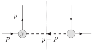
Refer to caption
Figure 1: Tree-level cut diagram for the calculation of T-even leading-twist parton densities. The dashed line indicates both scalar and axial-vector diquarks.

We assume the spectator to be point-like, with the quantum numbers of a diquark. Hence, the proton can couple to a quark and to a spectator diquark with spin 0 (scalar X=s𝑋𝑠X=s) or spin 1 (axial-vector X=a𝑋𝑎X=a), as well as with isospin 0 (isoscalar ud𝑢𝑑ud-like system) or isospin 1 (isovector uu𝑢𝑢uu-like system). Therefore, the tree-level “scattering amplitude” (0)superscript0\mathcal{M}^{(0)} is given by (see Fig. 1)

(0)(S)=Pp|ψ(0)|P,S={ip/m𝒴sU(P,S)scalar diquark,ip/mεμ(Pp,λa)𝒴aμU(P,S)axial-vector diquark,\mathcal{M}^{(0)}(S)=\langle P-p|\psi(0)|P,S\rangle=\ \begin{cases}\displaystyle{\frac{i}{\kern 1.99997ptp\kern-4.49997pt/-m}}\,{\cal Y}_{s}\,U(P,S)&\text{scalar diquark,}\\ \displaystyle{\frac{i}{\kern 1.99997ptp\kern-4.49997pt/-m}}\,\varepsilon^{*}_{\mu}(P-p,\lambda_{a})\,{\cal Y}^{\mu}_{a}\,U(P,S)&\text{axial-vector diquark,}\end{cases} (9)

and is actually a Dirac spinor because of the understood spinorial indices of the quark field ψ𝜓\psi. The εμ(Pp,λa)subscript𝜀𝜇𝑃𝑝subscript𝜆𝑎\varepsilon_{\mu}(P-p,\lambda_{a}) is the 4-vector polarization of the spin-1 vector diquark with momentum Pp𝑃𝑝P-p and helicity states λasubscript𝜆𝑎\lambda_{a}. When summing over all polarizations states, several choices have been used for dμν=λaε(λa)με(λa)νsuperscript𝑑𝜇𝜈subscriptsubscript𝜆𝑎subscriptsuperscript𝜀absent𝜇subscript𝜆𝑎subscriptsuperscript𝜀𝜈subscript𝜆𝑎d^{\mu\nu}=\sum_{\lambda_{a}}\varepsilon^{\ast\mu}_{(\lambda_{a})}\,\varepsilon^{\nu}_{(\lambda_{a})}:

dμν(Pp)={gμν+(Pp)μnν+(Pp)νnμ(Pp)nMa2[(Pp)n]2nμnν(see Ref. Brodsky:2000ii ),gμν+(Pp)μ(Pp)νMa2(see Ref. Gamberg:2007wm ),gμν+PμPνMa2(see Ref. Jakob:1997wg ),gμν(see Ref. Bacchetta:2003rz ).superscript𝑑𝜇𝜈𝑃𝑝casessuperscript𝑔𝜇𝜈superscript𝑃𝑝𝜇superscriptsubscript𝑛𝜈superscript𝑃𝑝𝜈superscriptsubscript𝑛𝜇𝑃𝑝subscript𝑛superscriptsubscript𝑀𝑎2superscriptdelimited-[]𝑃𝑝subscript𝑛2superscriptsubscript𝑛𝜇superscriptsubscript𝑛𝜈(see Ref. Brodsky:2000ii )superscript𝑔𝜇𝜈superscript𝑃𝑝𝜇superscript𝑃𝑝𝜈superscriptsubscript𝑀𝑎2(see Ref. Gamberg:2007wm ),superscript𝑔𝜇𝜈superscript𝑃𝜇superscript𝑃𝜈superscriptsubscript𝑀𝑎2(see Ref. Jakob:1997wg ),superscript𝑔𝜇𝜈(see Ref. Bacchetta:2003rz ).d^{\mu\nu}(P-p)=\left\{\begin{array}[]{cc}-g^{\mu\nu}+\displaystyle{\frac{(P-p)^{\mu}n_{-}^{\nu}+(P-p)^{\nu}n_{-}^{\mu}}{(P-p)\cdot n_{-}}}-\displaystyle{\frac{M_{a}^{2}}{[(P-p)\cdot n_{-}]^{2}}}\,n_{-}^{\mu}\,n_{-}^{\nu}&\quad\mbox{(see Ref.~{}\cite[cite]{\@@bibref{Authors Phrase1YearPhrase2}{Brodsky:2000ii}{\@@citephrase{(}}{\@@citephrase{)}}})},\\[11.38092pt] -g^{\mu\nu}+\displaystyle{\frac{(P-p)^{\mu}\,(P-p)^{\nu}}{M_{a}^{2}}}&\quad\mbox{(see Ref.~{}\cite[cite]{\@@bibref{Authors Phrase1YearPhrase2}{Gamberg:2007wm}{\@@citephrase{(}}{\@@citephrase{)}}}),}\\[11.38092pt] -g^{\mu\nu}+\displaystyle{\frac{P^{\mu}\,P^{\nu}}{M_{a}^{2}}}&\quad\mbox{(see Ref.~{}\cite[cite]{\@@bibref{Authors Phrase1YearPhrase2}{Jakob:1997wg}{\@@citephrase{(}}{\@@citephrase{)}}}),}\\[11.38092pt] -g^{\mu\nu}&\quad\mbox{(see Ref.~{}\cite[cite]{\@@bibref{Authors Phrase1YearPhrase2}{Bacchetta:2003rz}{\@@citephrase{(}}{\@@citephrase{)}}}).}\end{array}\right. (10)

The different forms for the diquark propagator correspond to different physical theories and lead to different results for the parton distribution functions. We have analyzed all of them except for the third one, which was extensively studied already in Ref. Jakob:1997wg . However, we think that the first one is preferable to the others. The motivation is that in the spectator model we have to take into account that the diquarks have an electric charge and can couple to the virtual photon in DIS. In other words, in this model the quarks are not the only charged partons in the proton: the diquarks are also charged partons and they have spin different from 1212\textstyle{\frac{1}{2}}. The scalar diquark couples only to longitudinally polarized photons and gives contribution to the structure function FLsubscript𝐹𝐿F_{L}. This leads to a violation of the Callan–Gross relation, but leaves unchanged the (leading-order) interpretation of the structure function FTsubscript𝐹𝑇F_{T} as a charge-weighted sum of quark distribution functions. This seems the best way to reduce the phenomenological impact of the problem represented by the presence of the diquarks. For the vector diquark, we checked that the same situation occurs when only the light-cone transverse polarization states of the diquark are propagated, i.e., when the first choice of Eq. (10) for the polarization sum is used. In the other cases, the diquark would give a contribution also to the structure function FTsubscript𝐹𝑇F_{T}. On top of this, we remark that the last choice of Eq. (10) for the polarization sum introduces unphysical polarization states of the vector diquark (see discussion in next section). In conclusion, in the following we shall consider only light-cone transverse polarizations of the diquark, make only a few comments on the other choices, and leave the complete list of results in the Appendices.
Refer to caption
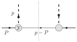
Figure 2: Tree-level cut diagram for the calculation of T-even leading-twist parton densities for an active scalar or vector diquark (dashed line), with a spectator quark (solid line).

Equation (9) can be further elaborated by choosing the nucleon-quark-diquark vertex 𝒴𝒴{\cal Y}. We choose the scalar and vector vertices to be

𝒴ssubscript𝒴𝑠\displaystyle{\cal Y}_{s} =igs(p2) 1l,absent𝑖subscript𝑔𝑠superscript𝑝21l\displaystyle=ig_{s}(p^{2})\,1\kern-3.00003pt{\rm l}\;, 𝒴aμsubscriptsuperscript𝒴𝜇𝑎\displaystyle{\cal Y}^{\mu}_{a} =iga(p2)2γμγ5,absent𝑖subscript𝑔𝑎superscript𝑝22superscript𝛾𝜇subscript𝛾5\displaystyle=i\frac{g_{a}(p^{2})}{\sqrt{2}}\,\gamma^{\mu}\,\gamma_{5}\,, (11)

where gX(p2)subscript𝑔𝑋superscript𝑝2g_{X}(p^{2}) is a suitable form factor. Other choices are possible (see, e.g., Refs Jakob:1997wg ; Gamberg:2007wm ), but we limit ourselves to these ones, which are the simplest. For the form factor, we explored three possible choices:

gX(p2)={gXp.l.point-like,gXdipp2m2|p2ΛX2|2dipolar,gXexpe(p2m2)/ΛX2exponential,subscript𝑔𝑋superscript𝑝2casessuperscriptsubscript𝑔𝑋formulae-sequence𝑝𝑙missing-subexpressionpoint-like,superscriptsubscript𝑔𝑋𝑑𝑖𝑝superscript𝑝2superscript𝑚2superscriptsuperscript𝑝2superscriptsubscriptΛ𝑋22missing-subexpressiondipolar,superscriptsubscript𝑔𝑋𝑒𝑥𝑝superscript𝑒superscript𝑝2superscript𝑚2superscriptsubscriptΛ𝑋2missing-subexpressionexponential,g_{X}(p^{2})=\left\{\begin{array}[]{ccl}g_{X}^{p.l.}&&\text{point-like,}\\[5.69046pt] g_{X}^{dip}\,\displaystyle{\frac{p^{2}-m^{2}}{{|p^{2}-\Lambda_{X}^{2}|}^{2}}}&&\text{dipolar,}\\[11.38092pt] g_{X}^{exp}\,e^{\,(p^{2}-m^{2})/\Lambda_{X}^{2}}&&\text{exponential,}\end{array}\right. (12)

where gXsubscript𝑔𝑋g_{X} and ΛXsubscriptΛ𝑋\Lambda_{X} are appropriate coupling constants and cutoffs, respectively, to be considered as free parameters of the model together with the mass of the diquark MXsubscript𝑀𝑋M_{X}. All these parameters can in principle be different for each type of diquark. Only the point-like coupling can be derived from a specific Lagrangian with protons, quarks and diquarks as fundamental degrees of freedom, and meant to effectively describe QCD in the nonperturbative regime. Since our interest here is mainly phenomenological, we prefer to introduce form factors. They smoothly suppress the influence of high 𝒑Tsubscript𝒑𝑇{\bm{p}}_{\scriptscriptstyle T} — where our theory cannot be trusted — and eliminate the logarithmic divergences arising after 𝒑Tsubscript𝒑𝑇{\bm{p}}_{\scriptscriptstyle T} integration when using a point-like coupling. For later use, we note that the dipolar form factor can be usefully rewritten, using Eq. (8), as

gX(p2)=gXdipp2m2|p2ΛX2|2=gXdip(p2m2)(1x)2(𝒑T2+LX2(ΛX2))2.subscript𝑔𝑋superscript𝑝2superscriptsubscript𝑔𝑋𝑑𝑖𝑝superscript𝑝2superscript𝑚2superscriptsuperscript𝑝2superscriptsubscriptΛ𝑋22superscriptsubscript𝑔𝑋𝑑𝑖𝑝superscript𝑝2superscript𝑚2superscript1𝑥2superscriptsuperscriptsubscript𝒑𝑇2superscriptsubscript𝐿𝑋2superscriptsubscriptΛ𝑋22g_{X}(p^{2})=g_{X}^{dip}\,\frac{p^{2}-m^{2}}{{|p^{2}-\Lambda_{X}^{2}|}^{2}}=g_{X}^{dip}\,\frac{(p^{2}-m^{2})\,(1-x)^{2}}{\left({\bm{p}}_{\scriptscriptstyle T}^{2}+L_{X}^{2}(\Lambda_{X}^{2})\right)^{2}}\;. (13)

In summary, we have analyzed in total nine combinations of nucleon-quark-diquark form factors and forms for the diquark propagator. As mentioned above, we will discuss analytical and numerical results involving the dipolar form factor and the first choice of Eq. (10) (transverse diquark polarizations only), listing the formulae for the other cases in the Appendices A and B. To keep the notation lighter, we will denote the coupling gXdipsuperscriptsubscript𝑔𝑋𝑑𝑖𝑝g_{X}^{dip} simply as gXsubscript𝑔𝑋g_{X} from now on.

II.2 Light-cone wave functions

A convenient way to compute parton distribution functions is by making use of light-cone wave functions (LCWFs), as done for instance in Ref. Brodsky:2000ii . For the scalar diquark, LCWFs can be defined as

ψλqλN(x,𝒑T)=p+(Pp)+u¯(p,λq)p2m2𝒴sU(P,λN),subscriptsuperscript𝜓subscript𝜆𝑁subscript𝜆𝑞𝑥subscript𝒑𝑇superscript𝑝superscript𝑃𝑝¯𝑢𝑝subscript𝜆𝑞superscript𝑝2superscript𝑚2subscript𝒴𝑠𝑈𝑃subscript𝜆𝑁\psi^{\lambda_{N}}_{\lambda_{q}}(x,\bm{p}_{\scriptscriptstyle T})=\sqrt{\frac{p^{+}}{(P-p)^{+}}}\,\frac{\bar{u}(p,\lambda_{q})}{p^{2}-m^{2}}\,{\cal Y}_{s}\,U(P,\lambda_{N})\;, (14)

where the indices λN,λq,subscript𝜆𝑁subscript𝜆𝑞\lambda_{N},\,\lambda_{q}, refer to the helicity of the nucleon and of the quark, respectively, and are constrained by angular momentum conservation to the “spin sum rule” λN=λq+Lzsubscript𝜆𝑁subscript𝜆𝑞subscript𝐿𝑧\lambda_{N}=\lambda_{q}+L_{z}, where Lzsubscript𝐿𝑧L_{z} is the projection of the relative orbital angular momentum between the quark and the diquark. We use the conventions of Ref. Lepage:1980fj (see also Ref. Meissner:2007rx ). In standard representation, the spinors can be written as

u(p,+)𝑢𝑝\displaystyle u(p,+) =123/2p+(2p++mpx+ipy2p+mpx+ipy),absent1superscript232superscript𝑝matrix2superscript𝑝𝑚subscript𝑝𝑥𝑖subscript𝑝𝑦2superscript𝑝𝑚subscript𝑝𝑥𝑖subscript𝑝𝑦\displaystyle=\frac{1}{\sqrt{2^{3/2}\,p^{+}}}\,\begin{pmatrix}\sqrt{2}\,p^{+}+m\\ \quad\ p_{x}+ip_{y}\quad\ \\ \sqrt{2}\,p^{+}-m\\ p_{x}+ip_{y}\end{pmatrix}\;, u(p,)𝑢𝑝\displaystyle u(p,-) =123/2p+(px+ipy2p++mpxipy2p++m),absent1superscript232superscript𝑝matrixsubscript𝑝𝑥𝑖subscript𝑝𝑦2superscript𝑝𝑚subscript𝑝𝑥𝑖subscript𝑝𝑦2superscript𝑝𝑚\displaystyle=\frac{1}{\sqrt{2^{3/2}\,p^{+}}}\,\begin{pmatrix}-p_{x}+ip_{y}\\ \sqrt{2}\,p^{+}+m\\ \quad\ p_{x}-ip_{y}\quad\ \\ -\sqrt{2}\,p^{+}+m\end{pmatrix}\;, (15)

and similarly for the nucleon spinors (changing p,m𝑝𝑚p,m, to P,M𝑃𝑀P,M, respectively). We obtain

ψ++(x,𝒑T)subscriptsuperscript𝜓𝑥subscript𝒑𝑇\displaystyle\psi^{+}_{+}(x,\bm{p}_{\scriptscriptstyle T}) =(m+xM)ϕ/xabsent𝑚𝑥𝑀italic-ϕ𝑥\displaystyle=(m+xM)\,\phi/x (Lz=0),subscript𝐿𝑧0\displaystyle(L_{z}=0), (16)
ψ+(x,𝒑T)subscriptsuperscript𝜓𝑥subscript𝒑𝑇\displaystyle\psi^{+}_{-}(x,\bm{p}_{\scriptscriptstyle T}) =(px+ipy)ϕ/xabsentsubscript𝑝𝑥𝑖subscript𝑝𝑦italic-ϕ𝑥\displaystyle=-(p_{x}+ip_{y})\,\phi/x (Lz=+1),subscript𝐿𝑧1\displaystyle(L_{z}=+1), (17)
ψ+(x,𝒑T)subscriptsuperscript𝜓𝑥subscript𝒑𝑇\displaystyle\psi^{-}_{+}(x,\bm{p}_{\scriptscriptstyle T}) =[ψ+(x,𝒑T)]absentsuperscriptdelimited-[]subscriptsuperscript𝜓𝑥subscript𝒑𝑇\displaystyle=-\left[\psi^{+}_{-}(x,\bm{p}_{\scriptscriptstyle T})\right]^{*} (Lz=1),subscript𝐿𝑧1\displaystyle(L_{z}=-1), (18)
ψ(x,𝒑T)subscriptsuperscript𝜓𝑥subscript𝒑𝑇\displaystyle\psi^{-}_{-}(x,\bm{p}_{\scriptscriptstyle T}) =ψ++(x,𝒑T)absentsubscriptsuperscript𝜓𝑥subscript𝒑𝑇\displaystyle=\psi^{+}_{+}(x,\bm{p}_{\scriptscriptstyle T}) (Lz=0),subscript𝐿𝑧0\displaystyle(L_{z}=0), (19)
ϕ(x,𝒑T2)italic-ϕ𝑥superscriptsubscript𝒑𝑇2\displaystyle\phi(x,\bm{p}_{\scriptscriptstyle T}^{2}) =gs1xx(1x)𝒑T2+Ls2(m2),absentsubscript𝑔𝑠1𝑥𝑥1𝑥superscriptsubscript𝒑𝑇2superscriptsubscript𝐿𝑠2superscript𝑚2\displaystyle=-\frac{g_{s}}{\sqrt{1-x}}\,\frac{x(1-x)}{\bm{p}_{\scriptscriptstyle T}^{2}+L_{s}^{2}(m^{2})}\;, (20)

which correspond to Eqs. (44,46) of Ref. Brodsky:2000ii .

For the vector diquark, LCWFs can be defined as

ψλqλaλN(x,𝒑T)=p+(Pp)+u¯(p,λq)p2m2εμ(Pp,λa)𝒴aμU(P,λN),subscriptsuperscript𝜓subscript𝜆𝑁subscript𝜆𝑞subscript𝜆𝑎𝑥subscript𝒑𝑇superscript𝑝superscript𝑃𝑝¯𝑢𝑝subscript𝜆𝑞superscript𝑝2superscript𝑚2subscriptsuperscript𝜀𝜇𝑃𝑝subscript𝜆𝑎subscriptsuperscript𝒴𝜇𝑎𝑈𝑃subscript𝜆𝑁\psi^{\lambda_{N}}_{\lambda_{q}\lambda_{a}}(x,\bm{p}_{\scriptscriptstyle T})=\sqrt{\frac{p^{+}}{(P-p)^{+}}}\,\frac{\bar{u}(p,\lambda_{q})}{p^{2}-m^{2}}\,\varepsilon^{*}_{\mu}(P-p,\lambda_{a})\,{\cal Y}^{\mu}_{a}\,U(P,\lambda_{N})\;, (21)

where the index λasubscript𝜆𝑎\lambda_{a} refers to the helicity of the vector diquark and is constrained by λN=λq+λa+Lzsubscript𝜆𝑁subscript𝜆𝑞subscript𝜆𝑎subscript𝐿𝑧\lambda_{N}=\lambda_{q}+\lambda_{a}+L_{z}. The light-cone transverse polarization vectors are given by Brodsky:2000ii

ε(Pp,+)𝜀𝑃𝑝\displaystyle\varepsilon(P-p,+) =[(Pp)x+i(Pp)y2(Pp)+,0,12,i2]=[px+ipy2(1x)P+,0,12,i2],absentsubscript𝑃𝑝𝑥𝑖subscript𝑃𝑝𝑦2superscript𝑃𝑝012𝑖2subscript𝑝𝑥𝑖subscript𝑝𝑦21𝑥superscript𝑃012𝑖2\displaystyle=\biggl{[}-\frac{(P-p)_{x}+i(P-p)_{y}}{\sqrt{2}\,(P-p)^{+}},0,-\frac{1}{\sqrt{2}},-\frac{i}{\sqrt{2}}\biggr{]}=\biggl{[}\frac{p_{x}+ip_{y}}{\sqrt{2}\,(1-x)\,P^{+}},0,-\frac{1}{\sqrt{2}},-\frac{i}{\sqrt{2}}\biggr{]}\;, (22)
ε(Pp,)𝜀𝑃𝑝\displaystyle\varepsilon(P-p,-) =[pxipy2(1x)P+,0,12,i2].absentsubscript𝑝𝑥𝑖subscript𝑝𝑦21𝑥superscript𝑃012𝑖2\displaystyle=\biggl{[}-\frac{p_{x}-ip_{y}}{\sqrt{2}\,(1-x)\,P^{+}},0,\frac{1}{\sqrt{2}},-\frac{i}{\sqrt{2}}\biggr{]}\;. (23)

They satisfy the usual properties111Note that (𝑷𝒑)𝜺(±)0𝑷𝒑𝜺plus-or-minus0(\bm{P}-\bm{p})\cdot\bm{\varepsilon}(\pm)\neq 0, since ε(±)𝜀plus-or-minus\varepsilon(\pm) do not describe transverse polarization with respect to the diquark momentum. ε(±)ε(±)=1𝜀plus-or-minussuperscript𝜀plus-or-minus1\varepsilon(\pm)\cdot\varepsilon^{*}(\pm)=-1, ε(±)ε()=0𝜀plus-or-minussuperscript𝜀minus-or-plus0\varepsilon(\pm)\cdot\varepsilon^{*}(\mp)=0, and (Pp)ε(±)=0𝑃𝑝𝜀plus-or-minus0(P-p)\cdot\varepsilon(\pm)=0. They are consistent with the polarization sum being expressed by the first option in Eq. (10). The LCWFs become

ψ+++(x,𝒑T)subscriptsuperscript𝜓absent𝑥subscript𝒑𝑇\displaystyle\psi^{+}_{++}(x,\bm{p}_{\scriptscriptstyle T}) =pxipy1xϕ/xabsentsubscript𝑝𝑥𝑖subscript𝑝𝑦1𝑥italic-ϕ𝑥\displaystyle=\frac{p_{x}-ip_{y}}{1-x}\,\phi/x (Lz=1),subscript𝐿𝑧1\displaystyle(L_{z}=-1), (24)
ψ++(x,𝒑T)subscriptsuperscript𝜓absent𝑥subscript𝒑𝑇\displaystyle\psi^{+}_{+-}(x,\bm{p}_{\scriptscriptstyle T}) =xpx+ipy1xϕ/xabsent𝑥subscript𝑝𝑥𝑖subscript𝑝𝑦1𝑥italic-ϕ𝑥\displaystyle=-x\,\frac{p_{x}+ip_{y}}{1-x}\,\phi/x (Lz=+1),subscript𝐿𝑧1\displaystyle(L_{z}=+1), (25)
ψ++(x,𝒑T)subscriptsuperscript𝜓absent𝑥subscript𝒑𝑇\displaystyle\psi^{+}_{-+}(x,\bm{p}_{\scriptscriptstyle T}) =(m+xM)ϕ/xabsent𝑚𝑥𝑀italic-ϕ𝑥\displaystyle=(m+xM)\,\phi/x (Lz=0),subscript𝐿𝑧0\displaystyle(L_{z}=0), (26)
ψ+(x,𝒑T)subscriptsuperscript𝜓absent𝑥subscript𝒑𝑇\displaystyle\psi^{+}_{--}(x,\bm{p}_{\scriptscriptstyle T}) =0absent0\displaystyle=0 (Lz=+2),subscript𝐿𝑧2\displaystyle(L_{z}=+2), (27)
ψ++(x,𝒑T)subscriptsuperscript𝜓absent𝑥subscript𝒑𝑇\displaystyle\psi^{-}_{++}(x,\bm{p}_{\scriptscriptstyle T}) =0absent0\displaystyle=0 (Lz=2),subscript𝐿𝑧2\displaystyle(L_{z}=-2), (28)
ψ+(x,𝒑T)subscriptsuperscript𝜓absent𝑥subscript𝒑𝑇\displaystyle\psi^{-}_{+-}(x,\bm{p}_{\scriptscriptstyle T}) =ψ++(x,𝒑T)absentsubscriptsuperscript𝜓absent𝑥subscript𝒑𝑇\displaystyle=-\psi^{+}_{-+}(x,\bm{p}_{\scriptscriptstyle T}) (Lz=0),subscript𝐿𝑧0\displaystyle(L_{z}=0), (29)
ψ+(x,𝒑T)subscriptsuperscript𝜓absent𝑥subscript𝒑𝑇\displaystyle\psi^{-}_{-+}(x,\bm{p}_{\scriptscriptstyle T}) =[ψ++(x,𝒑T)]absentsuperscriptdelimited-[]subscriptsuperscript𝜓absent𝑥subscript𝒑𝑇\displaystyle=\left[\psi^{+}_{+-}(x,\bm{p}_{\scriptscriptstyle T})\right]^{*} (Lz=1),subscript𝐿𝑧1\displaystyle(L_{z}=-1), (30)
ψ(x,𝒑T)subscriptsuperscript𝜓absent𝑥subscript𝒑𝑇\displaystyle\psi^{-}_{--}(x,\bm{p}_{\scriptscriptstyle T}) =[ψ+++(x,𝒑T)]absentsuperscriptdelimited-[]subscriptsuperscript𝜓absent𝑥subscript𝒑𝑇\displaystyle=\left[\psi^{+}_{++}(x,\bm{p}_{\scriptscriptstyle T})\right]^{*} (Lz=+1),subscript𝐿𝑧1\displaystyle(L_{z}=+1), (31)
ϕ(x,𝒑T2)italic-ϕ𝑥superscriptsubscript𝒑𝑇2\displaystyle\phi(x,\bm{p}_{\scriptscriptstyle T}^{2}) =ga1xx(1x)𝒑T2+La2(m2),absentsubscript𝑔𝑎1𝑥𝑥1𝑥superscriptsubscript𝒑𝑇2superscriptsubscript𝐿𝑎2superscript𝑚2\displaystyle=-\frac{g_{a}}{\sqrt{1-x}}\,\frac{x(1-x)}{\bm{p}_{\scriptscriptstyle T}^{2}+L_{a}^{2}(m^{2})}\;, (32)

and are analogous to Eqs. (21,24) in Ref. Brodsky:2000ii , the differences being due to the fact that here the diquark is an axial-vector particle rather than a vector one. Note that in our model we can only have wavefunctions with at most one unit of orbital angular momentum (p𝑝p wave). The LCWFs with two units of orbital angular momentum (d𝑑d-wave), ψ+subscriptsuperscript𝜓absent\psi^{+}_{--} and ψ++subscriptsuperscript𝜓absent\psi^{-}_{++}, vanish.

If we add to ε(Pp,±)𝜀𝑃𝑝plus-or-minus\varepsilon(P-p,\pm) also the third longitudinal polarization vector

ε(Pp,0)=1Ma[𝒑T2Ma22(1x)P+,(1x)P+,px,py],𝜀𝑃𝑝01subscript𝑀𝑎superscriptsubscript𝒑𝑇2superscriptsubscript𝑀𝑎221𝑥superscript𝑃1𝑥superscript𝑃subscript𝑝𝑥subscript𝑝𝑦\varepsilon(P-p,0)=\frac{1}{M_{a}}\biggl{[}\frac{\bm{p}_{\scriptscriptstyle T}^{2}-M_{a}^{2}}{2\,(1-x)\,P^{+}},(1-x)\,P^{+},-p_{x},-p_{y}\biggr{]}\;, (33)

satisfying222Note that 𝜺(0)𝜺0\bm{\varepsilon}(0) is not parallel to (𝑷𝒑)𝑷𝒑(\bm{P}-\bm{p}) because it describes longitudinal polarization states in the light-cone. ε(0)ε(0)=1𝜀0superscript𝜀01\varepsilon(0)\cdot\varepsilon^{*}(0)=-1, ε(0)ε(±)=0𝜀0superscript𝜀plus-or-minus0\varepsilon(0)\cdot\varepsilon^{*}(\pm)=0, and (Pp)ε(0)=0𝑃𝑝𝜀00(P-p)\cdot\varepsilon(0)=0, the corresponding additional LCWFs are

ψ+0+(x,𝒑T)subscriptsuperscript𝜓0𝑥subscript𝒑𝑇\displaystyle\psi^{+}_{+0}(x,\bm{p}_{\scriptscriptstyle T}) =𝒑T2xMa2mM(1x)22(1x)Maϕ/xabsentsuperscriptsubscript𝒑𝑇2𝑥superscriptsubscript𝑀𝑎2𝑚𝑀superscript1𝑥221𝑥subscript𝑀𝑎italic-ϕ𝑥\displaystyle=\frac{\bm{p}_{\scriptscriptstyle T}^{2}-xM_{a}^{2}-mM\,(1-x)^{2}}{\sqrt{2}\,(1-x)\,M_{a}}\,\phi/x (Lz=0),subscript𝐿𝑧0\displaystyle(L_{z}=0), (34)
ψ0+(x,𝒑T)subscriptsuperscript𝜓0𝑥subscript𝒑𝑇\displaystyle\psi^{+}_{-0}(x,\bm{p}_{\scriptscriptstyle T}) =(m+M)(px+ipy)2Maϕ/xabsent𝑚𝑀subscript𝑝𝑥𝑖subscript𝑝𝑦2subscript𝑀𝑎italic-ϕ𝑥\displaystyle=\frac{(m+M)\,(p_{x}+ip_{y})}{\sqrt{2}\,M_{a}}\,\phi/x (Lz=+1),subscript𝐿𝑧1\displaystyle(L_{z}=+1), (35)
ψ+0(x,𝒑T)subscriptsuperscript𝜓0𝑥subscript𝒑𝑇\displaystyle\psi^{-}_{+0}(x,\bm{p}_{\scriptscriptstyle T}) =[ψ0+(x,𝒑T)]ϕ/xabsentsuperscriptdelimited-[]subscriptsuperscript𝜓0𝑥subscript𝒑𝑇italic-ϕ𝑥\displaystyle=\left[\psi^{+}_{-0}(x,\bm{p}_{\scriptscriptstyle T})\right]^{*}\,\phi/x (Lz=1),subscript𝐿𝑧1\displaystyle(L_{z}=-1), (36)
ψ0(x,𝒑T)subscriptsuperscript𝜓0𝑥subscript𝒑𝑇\displaystyle\psi^{-}_{-0}(x,\bm{p}_{\scriptscriptstyle T}) =ψ+0+(x,𝒑T)ϕ/xabsentsubscriptsuperscript𝜓0𝑥subscript𝒑𝑇italic-ϕ𝑥\displaystyle=-\psi^{+}_{+0}(x,\bm{p}_{\scriptscriptstyle T})\,\phi/x\; (Lz=0).subscript𝐿𝑧0\displaystyle(L_{z}=0). (37)

From the above combinations we deduce, for example, that the proton with positive helicity +1212+\textstyle{\frac{1}{2}} can be in a state with probability density proportional to |ψ+|2superscriptsubscriptsuperscript𝜓2|\psi^{+}_{-}|^{2}, where the quark has opposite helicity and Lz=+1subscript𝐿𝑧1L_{z}=+1 orbital angular momentum with respect to a scalar diquark. This configuration is relativistically enhanced with respect to |ψ++|2superscriptsubscriptsuperscript𝜓2|\psi^{+}_{+}|^{2} with Lz=0subscript𝐿𝑧0L_{z}=0, where proton and quark helicities are aligned; thus, it suggests a possible explanation of the proton “spin puzzle” in terms of the relativistic aspects of the motion of quarks inside hadrons Brodsky:2000ii .

For the purpose of this work, it is also important to note that a nonvanishing relative orbital angular momentum between the quark and the diquark implies that the partons do not necessarily occupy the lowest-energy available orbital (with quantum numbers JP=12+superscript𝐽𝑃superscript12J^{P}={\textstyle{\frac{1}{2}}}^{+} and Lz=0subscript𝐿𝑧0L_{z}=0). Hence, in this version of the spectator diquark model the nucleon wave function does not show a SU(4)=SU(2)tensor-product\otimesSU(2) spin-isospin symmetry, contrary to what is usually assumed Jakob:1997wg .

Finally, we mention that the completeness relation for the last choice of the polarization sum in Eq. (10) should be written

λa=±,0εμ(Pp,λa)εν(Pp,λa)εμ(Pp,t)εν(Pp,t)=gμν,subscriptsubscript𝜆𝑎plus-or-minus0superscript𝜀absent𝜇𝑃𝑝subscript𝜆𝑎superscript𝜀𝜈𝑃𝑝subscript𝜆𝑎superscript𝜀absent𝜇𝑃𝑝𝑡superscript𝜀𝜈𝑃𝑝𝑡superscript𝑔𝜇𝜈\sum_{\lambda_{a}=\pm,0}\varepsilon^{\ast\mu}(P-p,\lambda_{a})\,\varepsilon^{\nu}(P-p,\lambda_{a})-\varepsilon^{\ast\mu}(P-p,t)\,\varepsilon^{\nu}(P-p,t)=-g^{\mu\nu}, (38)

where the unphysical time-like polarization state εμ(Pp,t)=(Pp)μ/Masuperscript𝜀𝜇𝑃𝑝𝑡superscript𝑃𝑝𝜇subscript𝑀𝑎\varepsilon^{\mu}(P-p,t)=(P-p)^{\mu}/M_{a} appears. The associated LCWFs read

ψ+t+(x,𝒑T)subscriptsuperscript𝜓𝑡𝑥subscript𝒑𝑇\displaystyle\psi^{+}_{+t}(x,\bm{p}_{\scriptscriptstyle T}) =𝒑T2+xMa2mM(1x)22(1+x)Maϕ/xabsentsuperscriptsubscript𝒑𝑇2𝑥superscriptsubscript𝑀𝑎2𝑚𝑀superscript1𝑥221𝑥subscript𝑀𝑎italic-ϕ𝑥\displaystyle=\frac{\bm{p}_{\scriptscriptstyle T}^{2}+xM_{a}^{2}-mM\,(1-x)^{2}}{\sqrt{2}\,(1+x)\,M_{a}}\,\phi/x (Lz=0),subscript𝐿𝑧0\displaystyle(L_{z}=0), (39)
ψt+(x,𝒑T)subscriptsuperscript𝜓𝑡𝑥subscript𝒑𝑇\displaystyle\psi^{+}_{-t}(x,\bm{p}_{\scriptscriptstyle T}) =(m+M)(px+ipy)2Maϕ/xabsent𝑚𝑀subscript𝑝𝑥𝑖subscript𝑝𝑦2subscript𝑀𝑎italic-ϕ𝑥\displaystyle=\frac{(m+M)\,(p_{x}+ip_{y})}{\sqrt{2}\,M_{a}}\,\phi/x (Lz=+1),subscript𝐿𝑧1\displaystyle(L_{z}=+1), (40)
ψ+t(x,𝒑T)subscriptsuperscript𝜓𝑡𝑥subscript𝒑𝑇\displaystyle\psi^{-}_{+t}(x,\bm{p}_{\scriptscriptstyle T}) =[ψt+(x,𝒑T)]ϕ/xabsentsuperscriptdelimited-[]subscriptsuperscript𝜓𝑡𝑥subscript𝒑𝑇italic-ϕ𝑥\displaystyle=\left[\psi^{+}_{-t}(x,\bm{p}_{\scriptscriptstyle T})\right]^{*}\,\phi/x (Lz=1),subscript𝐿𝑧1\displaystyle(L_{z}=-1), (41)
ψt(x,𝒑T)subscriptsuperscript𝜓𝑡𝑥subscript𝒑𝑇\displaystyle\psi^{-}_{-t}(x,\bm{p}_{\scriptscriptstyle T}) =ψ+t+(x,𝒑T)ϕ/xabsentsubscriptsuperscript𝜓𝑡𝑥subscript𝒑𝑇italic-ϕ𝑥\displaystyle=-\psi^{+}_{+t}(x,\bm{p}_{\scriptscriptstyle T})\,\phi/x (Lz=0).subscript𝐿𝑧0\displaystyle(L_{z}=0). (42)

II.3 T-even functions

The simplest example of T-even parton density is the unpolarized quark distribution f1(x,𝒑T)subscript𝑓1𝑥subscript𝒑𝑇f_{1}(x,{\bm{p}}_{\scriptscriptstyle T}), defined as

f1(x,𝒑T)=14Tr[(Φ(x,𝒑T,S)+Φ(x,𝒑T,S))γ+]+h.c.=141(2π)312(1x)P+Tr[(¯(0)(S)(0)(S)+¯(0)(S)(0)(S))γ+]+h.c..\begin{split}f_{1}(x,{\bm{p}}_{\scriptscriptstyle T})&=\frac{1}{4}\,\mathrm{Tr}\left[\left(\Phi(x,{\bm{p}}_{\scriptscriptstyle T},S)+\Phi(x,{\bm{p}}_{\scriptscriptstyle T},-S)\right)\,\gamma^{+}\right]+\mathrm{h.c.}\\ &=\frac{1}{4}\,\frac{1}{(2\pi)^{3}}\,\frac{1}{2(1-x)P^{+}}\,\mathrm{Tr}\left[\left(\overline{\mathcal{M}}^{(0)}(S)\,\mathcal{M}^{(0)}(S)+\overline{\mathcal{M}}^{(0)}(-S)\,\mathcal{M}^{(0)}(-S)\right)\,\gamma^{+}\right]+\mathrm{h.c.}\;.\end{split} (43)

By inserting in (0)superscript0\mathcal{M}^{(0)} of Eq. (9) the rules (11) for the nucleon-quark-diquark vertex, the dipolar form factor of Eq. (13), and the first choice in Eq. (10) for the sum of the polarization states of the diquark (transverse polarizations only), we get

f1q(s)(x,𝒑T)superscriptsubscript𝑓1𝑞𝑠𝑥subscript𝒑𝑇\displaystyle f_{1}^{q(s)}(x,{\bm{p}}_{\scriptscriptstyle T}) =gs2(2π)3[(m+xM)2+𝒑T2](1x)32[𝒑T2+Ls2(Λs2)]4absentsuperscriptsubscript𝑔𝑠2superscript2𝜋3delimited-[]superscript𝑚𝑥𝑀2superscriptsubscript𝒑𝑇2superscript1𝑥32superscriptdelimited-[]superscriptsubscript𝒑𝑇2superscriptsubscript𝐿𝑠2superscriptsubscriptΛ𝑠24\displaystyle=\frac{g_{s}^{2}}{(2\pi)^{3}}\,\frac{[(m+xM)^{2}+{\bm{p}}_{\scriptscriptstyle T}^{2}]\,(1-x)^{3}}{2\,[{\bm{p}}_{\scriptscriptstyle T}^{2}+L_{s}^{2}(\Lambda_{s}^{2})]^{4}} (44)
f1q(a)(x,𝒑T)superscriptsubscript𝑓1𝑞𝑎𝑥subscript𝒑𝑇\displaystyle f_{1}^{q(a)}(x,{\bm{p}}_{\scriptscriptstyle T}) =ga2(2π)3[𝒑T2(1+x2)+(m+xM)2(1x)2](1x)2[𝒑T2+La2(Λa2)]4.absentsuperscriptsubscript𝑔𝑎2superscript2𝜋3delimited-[]superscriptsubscript𝒑𝑇21superscript𝑥2superscript𝑚𝑥𝑀2superscript1𝑥21𝑥2superscriptdelimited-[]superscriptsubscript𝒑𝑇2superscriptsubscript𝐿𝑎2superscriptsubscriptΛ𝑎24\displaystyle=\frac{g_{a}^{2}}{(2\pi)^{3}}\,\frac{[{\bm{p}}_{\scriptscriptstyle T}^{2}\,(1+x^{2})+(m+xM)^{2}\,(1-x)^{2}]\,(1-x)}{2\,[{\bm{p}}_{\scriptscriptstyle T}^{2}+L_{a}^{2}(\Lambda_{a}^{2})]^{4}}\;. (45)

The same result can be recovered through the alternative definition

f1q(s)(x,𝒑T2)superscriptsubscript𝑓1𝑞𝑠𝑥superscriptsubscript𝒑𝑇2\displaystyle f_{1}^{q(s)}(x,\bm{p}_{\scriptscriptstyle T}^{2}) =116π312λN=±λq=±|ψλqλN|2=116π3(|ψ++|2+|ψ+|2)absent116superscript𝜋312subscriptsubscript𝜆𝑁plus-or-minussubscriptsubscript𝜆𝑞plus-or-minussuperscriptsubscriptsuperscript𝜓subscript𝜆𝑁subscript𝜆𝑞2116superscript𝜋3superscriptsubscriptsuperscript𝜓2superscriptsubscriptsuperscript𝜓2\displaystyle=\frac{1}{16\pi^{3}}\,\frac{1}{2}\sum_{\lambda_{N}=\pm}\,\sum_{\lambda_{q}=\pm}\,|\psi^{\lambda_{N}}_{\lambda_{q}}|^{2}=\frac{1}{16\pi^{3}}\Bigl{(}|\psi^{+}_{+}|^{2}+|\psi^{+}_{-}|^{2}\Bigr{)} (46)
f1q(a)(x,𝒑T2)superscriptsubscript𝑓1𝑞𝑎𝑥superscriptsubscript𝒑𝑇2\displaystyle f_{1}^{q(a)}(x,\bm{p}_{\scriptscriptstyle T}^{2}) =116π312λN=±λq=±λa=±|ψλqλaλN|2=116π3(|ψ+++|2+|ψ++|2+|ψ++|2+|ψ+|2),absent116superscript𝜋312subscriptsubscript𝜆𝑁plus-or-minussubscriptsubscript𝜆𝑞plus-or-minussubscriptsubscript𝜆𝑎plus-or-minussuperscriptsubscriptsuperscript𝜓subscript𝜆𝑁subscript𝜆𝑞subscript𝜆𝑎2116superscript𝜋3superscriptsubscriptsuperscript𝜓absent2superscriptsubscriptsuperscript𝜓absent2superscriptsubscriptsuperscript𝜓absent2superscriptsubscriptsuperscript𝜓absent2\displaystyle=\frac{1}{16\pi^{3}}\,\frac{1}{2}\sum_{\lambda_{N}=\pm}\,\sum_{\lambda_{q}=\pm}\,\sum_{\lambda_{a}=\pm}\,|\psi^{\lambda_{N}}_{\lambda_{q}\lambda_{a}}|^{2}=\frac{1}{16\pi^{3}}\Bigl{(}|\psi^{+}_{++}|^{2}+|\psi^{+}_{+-}|^{2}+|\psi^{+}_{-+}|^{2}+|\psi^{+}_{--}|^{2}\Bigr{)}\;, (47)

and replacing the results for the LCWFs using Eqs. (20) and (32) for the scalar and vector diquark, respectively.

If we use, instead, the second option of Eq. (10) for the sum over polarizations of the vector diquark (transverse and longitudinal polarizations), we obtain

f1q(a)(x,𝒑T)+116π3(|ψ+0+|2+|ψ0+|2).superscriptsubscript𝑓1𝑞𝑎𝑥subscript𝒑𝑇116superscript𝜋3superscriptsubscriptsuperscript𝜓02superscriptsubscriptsuperscript𝜓02f_{1}^{q(a)}(x,\bm{p}_{\scriptscriptstyle T})+\frac{1}{16\pi^{3}}\Bigl{(}|\psi^{+}_{+0}|^{2}+|\psi^{+}_{-0}|^{2}\Bigr{)}\;. (48)

The complete expression is given in Eq. (153) and corresponds to Eq. (10) of Ref. Gamberg:2007wm with Rg=0subscript𝑅𝑔0R_{g}=0.

Finally, the results with the last choice of Eq. (10) (transverse, longitudinal, and time-like polarizations) can be written as

f1q(a)(x,𝒑T)+116π3(|ψ+0+|2+|ψ0+|2)116π3(|ψ+t+|2+|ψt+|2).superscriptsubscript𝑓1𝑞𝑎𝑥subscript𝒑𝑇116superscript𝜋3superscriptsubscriptsuperscript𝜓02superscriptsubscriptsuperscript𝜓02116superscript𝜋3superscriptsubscriptsuperscript𝜓𝑡2superscriptsubscriptsuperscript𝜓𝑡2f_{1}^{q(a)}(x,\bm{p}_{\scriptscriptstyle T})+\frac{1}{16\pi^{3}}\Bigl{(}|\psi^{+}_{+0}|^{2}+|\psi^{+}_{-0}|^{2}\Bigr{)}-\frac{1}{16\pi^{3}}\Bigl{(}|\psi^{+}_{+t}|^{2}+|\psi^{+}_{-t}|^{2}\Bigr{)}\;. (49)

Note that the contribution of the diquark time-like polarization states enters with an overall negative sign. The complete expression is given in Eq. (157) and corresponds to Eq. (8) of Ref. Bacchetta:2003rz .

Turning back to our preferred choice, i.e.  the first option of Eq. (10) (light-cone transverse polarizations only), we now compute all other T-even, leading-twist TMDs. Their definition in terms of traces of the quark-quark correlator can be derived from, e.g., Eqs. (3.19) and ff. in Ref. Bacchetta:2006tn . To write them in terms of LCWFs, we need to introduce the polarization state in a generic direction 𝑺^T=(cosϕS,sinϕS)subscript^𝑺𝑇subscriptitalic-ϕ𝑆subscriptitalic-ϕ𝑆\hat{\bm{S}}_{\scriptscriptstyle T}=(\cos\phi_{S},\sin\phi_{S}) in the transverse plane

U(P,)𝑈𝑃\displaystyle U(P,\uparrow) =12(U(P,+)+eiϕSU(P,)),absent12𝑈𝑃superscript𝑒𝑖subscriptitalic-ϕ𝑆𝑈𝑃\displaystyle=\frac{1}{\sqrt{2}}\,\left(U(P,+)+e^{i\phi_{S}}U(P,-)\right)\;, (50)
U(P,)𝑈𝑃\displaystyle U(P,\downarrow) =12(U(P,+)+ei(ϕS+π)U(P,)).absent12𝑈𝑃superscript𝑒𝑖subscriptitalic-ϕ𝑆𝜋𝑈𝑃\displaystyle=\frac{1}{\sqrt{2}}\,\left(U(P,+)+e^{i(\phi_{S}+\pi)}U(P,-)\right)\;. (51)

For ϕS=0,π/2,subscriptitalic-ϕ𝑆0𝜋2\phi_{S}=0,\pi/2, we recover the (positive) polarizations along the x^^𝑥\hat{x} and y^^𝑦\hat{y} axis, respectively Barone:2003fy . For the quark, we will use similar decompositions and use the notation 𝑺^qTsubscript^𝑺𝑞𝑇\hat{\bm{S}}_{q\scriptscriptstyle T} and ϕSqsubscriptitalic-ϕsubscript𝑆𝑞\phi_{S_{q}}, i.e.,

u¯(p,)¯𝑢𝑝\displaystyle\bar{u}(p,\uparrow) =12(u¯(p,+)+eiϕSqu¯(p,)),absent12¯𝑢𝑝superscript𝑒𝑖subscriptitalic-ϕsubscript𝑆𝑞¯𝑢𝑝\displaystyle=\frac{1}{\sqrt{2}}\,\left(\bar{u}(p,+)+e^{-i\phi_{S_{q}}}\bar{u}(p,-)\right)\;, (52)
u¯(p,)¯𝑢𝑝\displaystyle\bar{u}(p,\downarrow) =12(u¯(p,+)+ei(ϕSq+π)u¯(p,)).absent12¯𝑢𝑝superscript𝑒𝑖subscriptitalic-ϕsubscript𝑆𝑞𝜋¯𝑢𝑝\displaystyle=\frac{1}{\sqrt{2}}\,\left(\bar{u}(p,+)+e^{-i(\phi_{S_{q}}+\pi)}\bar{u}(p,-)\right)\;. (53)

With this conventions and keeping in mind that λXsubscript𝜆𝑋\lambda_{X} is absent for the scalar diquark and λX=±subscript𝜆𝑋plus-or-minus\lambda_{X}=\pm for the vector diquark, we can write the TMDs in the following way

g1L(x,𝒑T)subscript𝑔1𝐿𝑥subscript𝒑𝑇\displaystyle g_{1L}(x,{\bm{p}}_{\scriptscriptstyle T}) =116π3λX(|ψ+λX+|2|ψλX+|2),absent116superscript𝜋3subscriptsubscript𝜆𝑋superscriptsubscriptsuperscript𝜓subscript𝜆𝑋2superscriptsubscriptsuperscript𝜓subscript𝜆𝑋2\displaystyle=\frac{1}{16\pi^{3}}\,\sum_{\lambda_{X}}\,\Bigl{(}|\psi^{+}_{+\lambda_{X}}|^{2}-|\psi^{+}_{-\lambda_{X}}|^{2}\Bigr{)}\;, (54)
𝒑T𝑺^TMg1T(x,𝒑T)subscript𝒑𝑇subscript^𝑺𝑇𝑀subscript𝑔1𝑇𝑥subscript𝒑𝑇\displaystyle\frac{{\bm{p}}_{\scriptscriptstyle T}\cdot\hat{\bm{S}}_{\scriptscriptstyle T}}{M}\,g_{1T}(x,{\bm{p}}_{\scriptscriptstyle T}) =116π3λX(|ψ+λX|2|ψλX|2)absent116superscript𝜋3subscriptsubscript𝜆𝑋superscriptsubscriptsuperscript𝜓subscript𝜆𝑋2superscriptsubscriptsuperscript𝜓subscript𝜆𝑋2\displaystyle=\frac{1}{16\pi^{3}}\,\sum_{\lambda_{X}}\,\Bigl{(}|\psi^{\uparrow}_{+\lambda_{X}}|^{2}-|\psi^{\uparrow}_{-\lambda_{X}}|^{2}\Bigr{)} (55)
𝒑T𝑺^qTMh1L(x,𝒑T)subscript𝒑𝑇subscript^𝑺𝑞𝑇𝑀superscriptsubscript1𝐿perpendicular-to𝑥subscript𝒑𝑇\displaystyle\frac{{\bm{p}}_{\scriptscriptstyle T}\cdot\hat{\bm{S}}_{q\scriptscriptstyle T}}{M}\,h_{1L}^{\perp}(x,{\bm{p}}_{\scriptscriptstyle T}) =116π3λX(|ψλX+|2|ψλX+|2),absent116superscript𝜋3subscriptsubscript𝜆𝑋superscriptsubscriptsuperscript𝜓absentsubscript𝜆𝑋2superscriptsubscriptsuperscript𝜓absentsubscript𝜆𝑋2\displaystyle=\frac{1}{16\pi^{3}}\,\sum_{\lambda_{X}}\,\Bigl{(}|\psi^{+}_{\uparrow\lambda_{X}}|^{2}-|\psi^{+}_{\downarrow\lambda_{X}}|^{2}\Bigr{)}\;, (56)
𝑺^T𝑺^qTh1T(x,𝒑T)subscript^𝑺𝑇subscript^𝑺𝑞𝑇subscript1𝑇𝑥subscript𝒑𝑇\displaystyle\hat{\bm{S}}_{\scriptscriptstyle T}\cdot\hat{\bm{S}}_{q\scriptscriptstyle T}\;h_{1T}(x,{\bm{p}}_{\scriptscriptstyle T}) +𝒑T𝑺^TM𝒑T𝑺^qTMh1T(x,𝒑T)=116π3λX(|ψλX|2|ψλX|2).subscript𝒑𝑇subscript^𝑺𝑇𝑀subscript𝒑𝑇subscript^𝑺𝑞𝑇𝑀superscriptsubscript1𝑇perpendicular-to𝑥subscript𝒑𝑇116superscript𝜋3subscriptsubscript𝜆𝑋superscriptsubscriptsuperscript𝜓absentsubscript𝜆𝑋2superscriptsubscriptsuperscript𝜓absentsubscript𝜆𝑋2\displaystyle+\frac{{\bm{p}}_{\scriptscriptstyle T}\cdot\hat{\bm{S}}_{\scriptscriptstyle T}}{M}\,\frac{\bm{p}_{\scriptscriptstyle T}\cdot\hat{\bm{S}}_{q\scriptscriptstyle T}}{M}\,h_{1T}^{\perp}(x,{\bm{p}}_{\scriptscriptstyle T})=\frac{1}{16\pi^{3}}\,\sum_{\lambda_{X}}\,\Bigl{(}|\psi^{\uparrow}_{\uparrow\lambda_{X}}|^{2}-|\psi^{\uparrow}_{\downarrow\lambda_{X}}|^{2}\Bigr{)}\;. (57)

The above results automatically fulfill positivity bounds Bacchetta:1999kz .

The explicit expressions are

g1Lq(s)(x,𝒑T2)superscriptsubscript𝑔1𝐿𝑞𝑠𝑥superscriptsubscript𝒑𝑇2\displaystyle g_{1L}^{q(s)}(x,{\bm{p}}_{\scriptscriptstyle T}^{2}) =gs2(2π)3[(m+xM)2𝒑T2](1x)32[𝒑T2+Ls2(Λs2)]4,absentsuperscriptsubscript𝑔𝑠2superscript2𝜋3delimited-[]superscript𝑚𝑥𝑀2superscriptsubscript𝒑𝑇2superscript1𝑥32superscriptdelimited-[]superscriptsubscript𝒑𝑇2superscriptsubscript𝐿𝑠2superscriptsubscriptΛ𝑠24\displaystyle=\frac{g_{s}^{2}}{(2\pi)^{3}}\,\frac{[(m+xM)^{2}-{\bm{p}}_{\scriptscriptstyle T}^{2}]\,(1-x)^{3}}{2\,[{\bm{p}}_{\scriptscriptstyle T}^{2}+L_{s}^{2}(\Lambda_{s}^{2})]^{4}}\;, (58)
g1Lq(a)(x,𝒑T2)superscriptsubscript𝑔1𝐿𝑞𝑎𝑥superscriptsubscript𝒑𝑇2\displaystyle g_{1L}^{q(a)}(x,{\bm{p}}_{\scriptscriptstyle T}^{2}) =ga2(2π)3[𝒑T2(1+x2)(m+xM)2(1x)2](1x)2[𝒑T2+La2(Λa2)]4,absentsuperscriptsubscript𝑔𝑎2superscript2𝜋3delimited-[]superscriptsubscript𝒑𝑇21superscript𝑥2superscript𝑚𝑥𝑀2superscript1𝑥21𝑥2superscriptdelimited-[]superscriptsubscript𝒑𝑇2superscriptsubscript𝐿𝑎2superscriptsubscriptΛ𝑎24\displaystyle=\frac{g_{a}^{2}}{(2\pi)^{3}}\,\frac{[{\bm{p}}_{\scriptscriptstyle T}^{2}\,(1+x^{2})-(m+xM)^{2}\,(1-x)^{2}]\,(1-x)}{2\,[{\bm{p}}_{\scriptscriptstyle T}^{2}+L_{a}^{2}(\Lambda_{a}^{2})]^{4}}\;, (59)
g1Tq(s)(x,𝒑T2)superscriptsubscript𝑔1𝑇𝑞𝑠𝑥superscriptsubscript𝒑𝑇2\displaystyle g_{1T}^{q(s)}(x,{\bm{p}}_{\scriptscriptstyle T}^{2}) =gs2(2π)3M(m+xM)(1x)3[𝒑T2+Ls2(Λs2)]4,absentsuperscriptsubscript𝑔𝑠2superscript2𝜋3𝑀𝑚𝑥𝑀superscript1𝑥3superscriptdelimited-[]superscriptsubscript𝒑𝑇2superscriptsubscript𝐿𝑠2superscriptsubscriptΛ𝑠24\displaystyle=\frac{g_{s}^{2}}{(2\pi)^{3}}\,\frac{M\,(m+xM)\,(1-x)^{3}}{[{\bm{p}}_{\scriptscriptstyle T}^{2}+L_{s}^{2}(\Lambda_{s}^{2})]^{4}}\;, (60)
g1Tq(a)(x,𝒑T2)superscriptsubscript𝑔1𝑇𝑞𝑎𝑥superscriptsubscript𝒑𝑇2\displaystyle g_{1T}^{q(a)}(x,{\bm{p}}_{\scriptscriptstyle T}^{2}) =ga2(2π)3xM(m+xM)(1x)2[𝒑T2+La2(Λa2)]4,absentsuperscriptsubscript𝑔𝑎2superscript2𝜋3𝑥𝑀𝑚𝑥𝑀superscript1𝑥2superscriptdelimited-[]superscriptsubscript𝒑𝑇2superscriptsubscript𝐿𝑎2superscriptsubscriptΛ𝑎24\displaystyle=\frac{g_{a}^{2}}{(2\pi)^{3}}\,\frac{xM\,(m+xM)\,(1-x)^{2}}{[{\bm{p}}_{\scriptscriptstyle T}^{2}+L_{a}^{2}(\Lambda_{a}^{2})]^{4}}\;, (61)
h1Lq(s)(x,𝒑T2)superscriptsubscript1𝐿perpendicular-toabsent𝑞𝑠𝑥superscriptsubscript𝒑𝑇2\displaystyle h_{1L}^{\perp\,q(s)}(x,{\bm{p}}_{\scriptscriptstyle T}^{2}) =gs2(2π)3M(m+xM)(1x)3[𝒑T2+Ls2(Λs2)]4,absentsuperscriptsubscript𝑔𝑠2superscript2𝜋3𝑀𝑚𝑥𝑀superscript1𝑥3superscriptdelimited-[]superscriptsubscript𝒑𝑇2superscriptsubscript𝐿𝑠2superscriptsubscriptΛ𝑠24\displaystyle=-\frac{g_{s}^{2}}{(2\pi)^{3}}\,\frac{M\,(m+xM)\,(1-x)^{3}}{[{\bm{p}}_{\scriptscriptstyle T}^{2}+L_{s}^{2}(\Lambda_{s}^{2})]^{4}}\;, (62)
h1Lq(a)(x,𝒑T2)superscriptsubscript1𝐿perpendicular-toabsent𝑞𝑎𝑥superscriptsubscript𝒑𝑇2\displaystyle h_{1L}^{\perp\,q(a)}(x,{\bm{p}}_{\scriptscriptstyle T}^{2}) =ga2(2π)3M(m+xM)(1x)2[𝒑T2+La2(Λa2)]4,absentsuperscriptsubscript𝑔𝑎2superscript2𝜋3𝑀𝑚𝑥𝑀superscript1𝑥2superscriptdelimited-[]superscriptsubscript𝒑𝑇2superscriptsubscript𝐿𝑎2superscriptsubscriptΛ𝑎24\displaystyle=\frac{g_{a}^{2}}{(2\pi)^{3}}\,\frac{M\,(m+xM)\,(1-x)^{2}}{[{\bm{p}}_{\scriptscriptstyle T}^{2}+L_{a}^{2}(\Lambda_{a}^{2})]^{4}}\;, (63)
h1Tq(s)(x,𝒑T2)superscriptsubscript1𝑇𝑞𝑠𝑥superscriptsubscript𝒑𝑇2\displaystyle h_{1T}^{q(s)}(x,{\bm{p}}_{\scriptscriptstyle T}^{2}) =gs2(2π)3[𝒑T2+(m+xM)2](1x)32[𝒑T2+Ls2(Λs2)]4,absentsuperscriptsubscript𝑔𝑠2superscript2𝜋3delimited-[]superscriptsubscript𝒑𝑇2superscript𝑚𝑥𝑀2superscript1𝑥32superscriptdelimited-[]superscriptsubscript𝒑𝑇2superscriptsubscript𝐿𝑠2superscriptsubscriptΛ𝑠24\displaystyle=\frac{g_{s}^{2}}{(2\pi)^{3}}\,\frac{[{\bm{p}}_{\scriptscriptstyle T}^{2}+(m+xM)^{2}]\,(1-x)^{3}}{2\,[{\bm{p}}_{\scriptscriptstyle T}^{2}+L_{s}^{2}(\Lambda_{s}^{2})]^{4}}\>, (64)
h1Tq(a)(x,𝒑T2)superscriptsubscript1𝑇𝑞𝑎𝑥superscriptsubscript𝒑𝑇2\displaystyle h_{1T}^{q(a)}(x,{\bm{p}}_{\scriptscriptstyle T}^{2}) =ga2(2π)3𝒑T2x(1x)[𝒑T2+La2(Λa2)]4,absentsuperscriptsubscript𝑔𝑎2superscript2𝜋3superscriptsubscript𝒑𝑇2𝑥1𝑥superscriptdelimited-[]superscriptsubscript𝒑𝑇2superscriptsubscript𝐿𝑎2superscriptsubscriptΛ𝑎24\displaystyle=-\frac{g_{a}^{2}}{(2\pi)^{3}}\,\frac{{\bm{p}}_{\scriptscriptstyle T}^{2}\,x(1-x)}{[{\bm{p}}_{\scriptscriptstyle T}^{2}+L_{a}^{2}(\Lambda_{a}^{2})]^{4}}\;, (65)
h1Tq(s)(x,𝒑T2)superscriptsubscript1𝑇perpendicular-toabsent𝑞𝑠𝑥superscriptsubscript𝒑𝑇2\displaystyle h_{1T}^{\perp\,q(s)}(x,{\bm{p}}_{\scriptscriptstyle T}^{2}) =gs2(2π)3M2(1x)3[𝒑T2+Ls2(Λs2)]4,absentsuperscriptsubscript𝑔𝑠2superscript2𝜋3superscript𝑀2superscript1𝑥3superscriptdelimited-[]superscriptsubscript𝒑𝑇2superscriptsubscript𝐿𝑠2superscriptsubscriptΛ𝑠24\displaystyle=-\frac{g_{s}^{2}}{(2\pi)^{3}}\,\frac{M^{2}\,(1-x)^{3}}{[{\bm{p}}_{\scriptscriptstyle T}^{2}+L_{s}^{2}(\Lambda_{s}^{2})]^{4}}\;, (66)
h1Tq(a)(x,𝒑T2)superscriptsubscript1𝑇perpendicular-toabsent𝑞𝑎𝑥superscriptsubscript𝒑𝑇2\displaystyle h_{1T}^{\perp\,q(a)}(x,{\bm{p}}_{\scriptscriptstyle T}^{2}) =0.absent0\displaystyle=0\;. (67)

From the last two formulae we deduce also the expressions for the transversity distribution:

h1q(s)(x,𝒑T2)superscriptsubscript1𝑞𝑠𝑥superscriptsubscript𝒑𝑇2\displaystyle h_{1}^{q(s)}(x,{\bm{p}}_{\scriptscriptstyle T}^{2}) =h1Tq(s)(x,𝒑T2)+𝒑T22M2h1Tq(s)(x,𝒑T2)=gs2(2π)3(m+xM)2(1x)32[𝒑T2+Ls2(Λs2)]4absentsuperscriptsubscript1𝑇𝑞𝑠𝑥superscriptsubscript𝒑𝑇2superscriptsubscript𝒑𝑇22superscript𝑀2superscriptsubscript1𝑇perpendicular-toabsent𝑞𝑠𝑥superscriptsubscript𝒑𝑇2superscriptsubscript𝑔𝑠2superscript2𝜋3superscript𝑚𝑥𝑀2superscript1𝑥32superscriptdelimited-[]superscriptsubscript𝒑𝑇2superscriptsubscript𝐿𝑠2superscriptsubscriptΛ𝑠24\displaystyle=h_{1T}^{q(s)}(x,{\bm{p}}_{\scriptscriptstyle T}^{2})+\frac{{\bm{p}}_{\scriptscriptstyle T}^{2}}{2M^{2}}\,h_{1T}^{\perp\,q(s)}(x,{\bm{p}}_{\scriptscriptstyle T}^{2})=\frac{g_{s}^{2}}{(2\pi)^{3}}\,\frac{(m+xM)^{2}\,(1-x)^{3}}{2\,[{\bm{p}}_{\scriptscriptstyle T}^{2}+L_{s}^{2}(\Lambda_{s}^{2})]^{4}} (68)
h1q(a)(x,𝒑T2)superscriptsubscript1𝑞𝑎𝑥superscriptsubscript𝒑𝑇2\displaystyle h_{1}^{q(a)}(x,{\bm{p}}_{\scriptscriptstyle T}^{2}) =ga2(2π)3𝒑T2x(1x)[𝒑T2+La2(Λa2)]4.absentsuperscriptsubscript𝑔𝑎2superscript2𝜋3superscriptsubscript𝒑𝑇2𝑥1𝑥superscriptdelimited-[]superscriptsubscript𝒑𝑇2superscriptsubscript𝐿𝑎2superscriptsubscriptΛ𝑎24\displaystyle=-\frac{g_{a}^{2}}{(2\pi)^{3}}\,\frac{{\bm{p}}_{\scriptscriptstyle T}^{2}\,x(1-x)}{[{\bm{p}}_{\scriptscriptstyle T}^{2}+L_{a}^{2}(\Lambda_{a}^{2})]^{4}}\;. (69)

Note that the functions g1Tsubscript𝑔1𝑇g_{1T} and h1Lsuperscriptsubscript1𝐿perpendicular-toh_{1L}^{\perp} arise from the interference of LCWFs with |Lz|=1subscript𝐿𝑧1|L_{z}|=1 and Lz=0subscript𝐿𝑧0L_{z}=0. The function h1Tsuperscriptsubscript1𝑇perpendicular-toh_{1T}^{\perp} requires the interference of two LCWFs that differ by two units of Lzsubscript𝐿𝑧L_{z}. This condition is necessary but not sufficient to have h1T0superscriptsubscript1𝑇perpendicular-to0h_{1T}^{\perp}\neq 0. In fact, the vector diquark spectator gives h1T=0superscriptsubscript1𝑇perpendicular-to0h_{1T}^{\perp}=0 even if LCWFs with Lz=±1subscript𝐿𝑧plus-or-minus1L_{z}=\pm 1 are present.

Some interesting relations can be evinced from the above expressions. For example, the transversity with scalar diquark saturates the Soffer bound, while for axial-vector diquarks the relation is more involved:

h1q(s)(x,𝒑T2)superscriptsubscript1𝑞𝑠𝑥superscriptsubscript𝒑𝑇2\displaystyle h_{1}^{q(s)}(x,{\bm{p}}_{\scriptscriptstyle T}^{2}) =12(f1q(s)(x,𝒑T2)+g1q(s)(x,𝒑T2)),absent12superscriptsubscript𝑓1𝑞𝑠𝑥superscriptsubscript𝒑𝑇2superscriptsubscript𝑔1𝑞𝑠𝑥superscriptsubscript𝒑𝑇2\displaystyle=\frac{1}{2}\,\left(f_{1}^{q(s)}(x,{\bm{p}}_{\scriptscriptstyle T}^{2})+g_{1}^{q(s)}(x,{\bm{p}}_{\scriptscriptstyle T}^{2})\right)\;, (70)
h1q(a)(x,𝒑T2)superscriptsubscript1𝑞𝑎𝑥superscriptsubscript𝒑𝑇2\displaystyle h_{1}^{q(a)}(x,{\bm{p}}_{\scriptscriptstyle T}^{2}) =x1+x212(f1q(a)(x,𝒑T2)+g1q(a)(x,𝒑T2)).absent𝑥1superscript𝑥212superscriptsubscript𝑓1𝑞𝑎𝑥superscriptsubscript𝒑𝑇2superscriptsubscript𝑔1𝑞𝑎𝑥superscriptsubscript𝒑𝑇2\displaystyle=-\frac{x}{1+x^{2}}\,\frac{1}{2}\,\left(f_{1}^{q(a)}(x,{\bm{p}}_{\scriptscriptstyle T}^{2})+g_{1}^{q(a)}(x,{\bm{p}}_{\scriptscriptstyle T}^{2})\right)\;. (71)

When restricting to the results with scalar diquark, the g1Tsubscript𝑔1𝑇g_{1T} distribution is connected to two other partners by the relations

g1Tq(s)(x,𝒑T2)superscriptsubscript𝑔1𝑇𝑞𝑠𝑥superscriptsubscript𝒑𝑇2\displaystyle g_{1T}^{q(s)}(x,{\bm{p}}_{\scriptscriptstyle T}^{2}) =h1Lq(s)(x,𝒑T2),absentsuperscriptsubscript1𝐿perpendicular-toabsent𝑞𝑠𝑥superscriptsubscript𝒑𝑇2\displaystyle=-h_{1L}^{\perp\,q(s)}(x,{\bm{p}}_{\scriptscriptstyle T}^{2})\;, g1Tq(s)(x,𝒑T2)superscriptsubscript𝑔1𝑇𝑞𝑠𝑥superscriptsubscript𝒑𝑇2\displaystyle g_{1T}^{q(s)}(x,{\bm{p}}_{\scriptscriptstyle T}^{2}) =2Mm+xMh1q(s)(x,𝒑T2),absent2𝑀𝑚𝑥𝑀superscriptsubscript1𝑞𝑠𝑥superscriptsubscript𝒑𝑇2\displaystyle=\frac{2M}{m+xM}\,h_{1}^{q(s)}(x,{\bm{p}}_{\scriptscriptstyle T}^{2})\;, (72)

while for axial-vector diquarks we have

g1Tq(a)(x,𝒑T2)=xh1Lq(a)(x,𝒑T2).superscriptsubscript𝑔1𝑇𝑞𝑎𝑥superscriptsubscript𝒑𝑇2𝑥superscriptsubscript1𝐿perpendicular-toabsent𝑞𝑎𝑥superscriptsubscript𝒑𝑇2g_{1T}^{q(a)}(x,{\bm{p}}_{\scriptscriptstyle T}^{2})=x\,h_{1L}^{\perp\,q(a)}(x,{\bm{p}}_{\scriptscriptstyle T}^{2})\;. (73)

This relation is however different when considering spectator diquarks with more degrees of freedom (see App. A). Our results seem to indicate that no general relation exists between g1Tsubscript𝑔1𝑇g_{1T} and h1Lsuperscriptsubscript1𝐿perpendicular-toh_{1L}^{\perp}, contrary to what is proposed in Ref. Pasquini:2008ax . The reason is connected to the difference between LCWFs with Lz=1subscript𝐿𝑧1L_{z}=1 and Lz=1subscript𝐿𝑧1L_{z}=-1, as in Eqs. (24) and (25). We also observe that in the vector-diquark case g1Lh1subscript𝑔1𝐿subscript1g_{1L}-h_{1} and h1Tsuperscriptsubscript1𝑇perpendicular-toh_{1T}^{\perp} are not simply related through the relation suggested in Ref. Avakian:2008dz . We are led to conclude that such a relation is not general.

The 𝒑Tsubscript𝒑𝑇{\bm{p}}_{\scriptscriptstyle T}-integrated results are

f1q(s)(x)superscriptsubscript𝑓1𝑞𝑠𝑥\displaystyle f_{1}^{q(s)}(x) =gs2(2π)2[2(m+xM)2+Ls2(Λs2)](1x)324Ls6(Λs2)absentsuperscriptsubscript𝑔𝑠2superscript2𝜋2delimited-[]2superscript𝑚𝑥𝑀2superscriptsubscript𝐿𝑠2superscriptsubscriptΛ𝑠2superscript1𝑥324superscriptsubscript𝐿𝑠6superscriptsubscriptΛ𝑠2\displaystyle=\frac{g_{s}^{2}}{(2\pi)^{2}}\,\frac{[2\,(m+xM)^{2}+L_{s}^{2}(\Lambda_{s}^{2})]\,(1-x)^{3}}{24\,L_{s}^{6}(\Lambda_{s}^{2})} (74)
f1q(a)(x)superscriptsubscript𝑓1𝑞𝑎𝑥\displaystyle f_{1}^{q(a)}(x) =ga2(2π)2[2(m+xM)2(1x)2+(1+x2)La2(Λa2)](1x)24La6(Λa2)absentsuperscriptsubscript𝑔𝑎2superscript2𝜋2delimited-[]2superscript𝑚𝑥𝑀2superscript1𝑥21superscript𝑥2superscriptsubscript𝐿𝑎2superscriptsubscriptΛ𝑎21𝑥24superscriptsubscript𝐿𝑎6superscriptsubscriptΛ𝑎2\displaystyle=\frac{g_{a}^{2}}{(2\pi)^{2}}\,\frac{[2\,(m+xM)^{2}\,(1-x)^{2}+(1+x^{2})\,L_{a}^{2}(\Lambda_{a}^{2})]\,(1-x)}{24\,L_{a}^{6}(\Lambda_{a}^{2})} (75)
g1q(s)(x)superscriptsubscript𝑔1𝑞𝑠𝑥\displaystyle g_{1}^{q(s)}(x) =gs2(2π)2[2(m+xM)2Ls2(Λs2)](1x)324Ls6(Λs2)absentsuperscriptsubscript𝑔𝑠2superscript2𝜋2delimited-[]2superscript𝑚𝑥𝑀2superscriptsubscript𝐿𝑠2superscriptsubscriptΛ𝑠2superscript1𝑥324superscriptsubscript𝐿𝑠6superscriptsubscriptΛ𝑠2\displaystyle=\frac{g_{s}^{2}}{(2\pi)^{2}}\,\frac{[2\,(m+xM)^{2}-L_{s}^{2}(\Lambda_{s}^{2})]\,(1-x)^{3}}{24\,L_{s}^{6}(\Lambda_{s}^{2})} (76)
g1q(a)(x)superscriptsubscript𝑔1𝑞𝑎𝑥\displaystyle g_{1}^{q(a)}(x) =ga2(2π)2[2(m+xM)2(1x)2(1+x2)La2(Λa2)](1x)24La6(Λa2)absentsuperscriptsubscript𝑔𝑎2superscript2𝜋2delimited-[]2superscript𝑚𝑥𝑀2superscript1𝑥21superscript𝑥2superscriptsubscript𝐿𝑎2superscriptsubscriptΛ𝑎21𝑥24superscriptsubscript𝐿𝑎6superscriptsubscriptΛ𝑎2\displaystyle=-\frac{g_{a}^{2}}{(2\pi)^{2}}\,\frac{[2\,(m+xM)^{2}\,(1-x)^{2}-(1+x^{2})\,L_{a}^{2}(\Lambda_{a}^{2})]\,(1-x)}{24\,L_{a}^{6}(\Lambda_{a}^{2})} (77)
h1q(s)(x)superscriptsubscript1𝑞𝑠𝑥\displaystyle h_{1}^{q(s)}(x) =gs2(2π)2(m+xM)2(1x)312Ls6(Λs2)absentsuperscriptsubscript𝑔𝑠2superscript2𝜋2superscript𝑚𝑥𝑀2superscript1𝑥312superscriptsubscript𝐿𝑠6superscriptsubscriptΛ𝑠2\displaystyle=\frac{g_{s}^{2}}{(2\pi)^{2}}\,\frac{(m+xM)^{2}\,(1-x)^{3}}{12\,L_{s}^{6}(\Lambda_{s}^{2})} (78)
h1q(a)(x)superscriptsubscript1𝑞𝑎𝑥\displaystyle h_{1}^{q(a)}(x) =ga2(2π)2x(1x)12La4(Λa2).absentsuperscriptsubscript𝑔𝑎2superscript2𝜋2𝑥1𝑥12superscriptsubscript𝐿𝑎4superscriptsubscriptΛ𝑎2\displaystyle=-\frac{g_{a}^{2}}{(2\pi)^{2}}\,\frac{x(1-x)}{12\,L_{a}^{4}(\Lambda_{a}^{2})}\;. (79)

II.4 T-odd functions

The two leading-twist T-odd structures are the Sivers and Boer-Mulders distributions. They are defined as

εTijpTiSTjMf1T(x,𝒑T2)superscriptsubscript𝜀𝑇𝑖𝑗subscript𝑝𝑇𝑖subscript𝑆𝑇𝑗𝑀superscriptsubscript𝑓1𝑇perpendicular-to𝑥superscriptsubscript𝒑𝑇2\displaystyle\frac{\varepsilon_{\scriptscriptstyle T}^{ij}p_{\scriptscriptstyle Ti}S_{\scriptscriptstyle Tj}}{M}\,f_{1T}^{\perp}(x,{\bm{p}}_{\scriptscriptstyle T}^{2}) =14Tr[(Φ(x,𝒑T,S)Φ(x,𝒑T,S))γ+]+h.c.,formulae-sequenceabsent14Trdelimited-[]Φ𝑥subscript𝒑𝑇𝑆Φ𝑥subscript𝒑𝑇𝑆superscript𝛾hc\displaystyle=-\frac{1}{4}\,\mathrm{Tr}\left[\left(\Phi(x,{\bm{p}}_{\scriptscriptstyle T},S)-\Phi(x,{\bm{p}}_{\scriptscriptstyle T},-S)\right)\,\gamma^{+}\right]+\mathrm{h.c.}\;, (80)
εTijpTjMh1(x,𝒑T2)superscriptsubscript𝜀𝑇𝑖𝑗subscript𝑝𝑇𝑗𝑀superscriptsubscript1perpendicular-to𝑥superscriptsubscript𝒑𝑇2\displaystyle\frac{\varepsilon_{\scriptscriptstyle T}^{ij}p_{\scriptscriptstyle Tj}}{M}\,h_{1}^{\perp}(x,{\bm{p}}_{\scriptscriptstyle T}^{2}) =14Tr[(Φ(x,𝒑T,S)+Φ(x,𝒑T,S))iσi+γ5]+h.c..formulae-sequenceabsent14Trdelimited-[]Φ𝑥subscript𝒑𝑇𝑆Φ𝑥subscript𝒑𝑇𝑆𝑖superscript𝜎limit-from𝑖subscript𝛾5hc\displaystyle=\frac{1}{4}\,\mathrm{Tr}\left[\left(\Phi(x,{\bm{p}}_{\scriptscriptstyle T},S)+\Phi(x,{\bm{p}}_{\scriptscriptstyle T},-S)\right)\,i\sigma^{i+}\,\gamma_{5}\right]+\mathrm{h.c.}\;. (81)

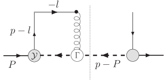
At tree level, these expressions vanish because there is no residual interaction between the active quark and the spectators; equivalently, there is no interference between two competing channels producing the complex amplitude whose imaginary part gives the T-odd contribution. We can generate such structures by considering the interference between the tree-level scattering amplitude and the single-gluon-exchange scattering amplitude in eikonal approximation, as shown in Fig. 3 (the Hermitean conjugate partner must also be considered). This corresponds just to the leading-twist one-gluon-exchange approximation of the gauge link operator of Eq. (5Boer:2003cm .

Refer to caption
Figure 3: Interference between the one-gluon exchange diagram in eikonal approximation and the tree level diagram in the spectator model. The Hermitean conjugate diagram is not shown.

For the moment, we use Abelian gluons. The QCD color structure will be recovered at the end. The Feynman rules to be used for the eikonal vertex and propagator are Collins:1981uk ; Collins:1982uw

=iecnρ,absent𝑖subscript𝑒𝑐superscriptsubscript𝑛𝜌\displaystyle=-ie_{c}\,n_{-}^{\rho}\,, [Uncaptioned image] =il++iϵ,absent𝑖superscript𝑙𝑖italic-ϵ\displaystyle=\frac{i}{-l^{+}+i\epsilon}\,, (82)

where ecsubscript𝑒𝑐e_{c} is the color charge of the quark and the sign of iϵ𝑖italic-ϵi\epsilon for the eikonal line corresponds to the gauge link of SIDIS. In cut diagrams one must take the complex conjugate of these expressions for vertices and propagators on the right of the final-state cut.

The explicit form of the contribution Φ(1)superscriptΦ1\Phi^{(1)} to the correlation function corresponding to Fig. 3 is

Φ(1)(x,𝒑T,S)1(2π)312(1x)P+(¯(0)(S)(1)(S)+¯(1)(S)(0)(S))|p2=τ(x,𝒑T),similar-tosuperscriptΦ1𝑥subscript𝒑𝑇𝑆evaluated-at1superscript2𝜋3121𝑥superscript𝑃superscript¯0𝑆superscript1𝑆superscript¯1𝑆superscript0𝑆superscript𝑝2𝜏𝑥subscript𝒑𝑇\Phi^{(1)}(x,{\bm{p}}_{\scriptscriptstyle T},S)\sim\frac{1}{(2\pi)^{3}}\,\frac{1}{2(1-x)P^{+}}\,\Bigl{(}\overline{\mathcal{M}}^{(0)}(S)\,\mathcal{M}^{(1)}(S)+\overline{\mathcal{M}}^{(1)}(S)\,\mathcal{M}^{(0)}(S)\Bigr{)}\Big{|}_{p^{2}=\tau(x,{\bm{p}}_{{}_{T}})}\;, (83)

where τ(x,𝒑T)𝜏𝑥subscript𝒑𝑇\tau(x,{\bm{p}}_{{}_{\scriptscriptstyle T}}) is defined in Eq. (8) and

(1)(S)={d4l(2π)4iecΓsρnρ(p/l/+m)𝒴sU(P,S)(D1+iε)(D2iε)(D3+iε)(D4+iε)scalar diquark,d4l(2π)4iecεσ(Pp,λa)Γaρνσnρ(p/l/+m)dμν(plP)𝒴aμU(P,S)(D1+iε)(D2iε)(D3+iε)(D4+iε)axial-vector diquark,\mathcal{M}^{(1)}(S)=\begin{cases}\displaystyle{-\int\frac{d^{4}l}{(2\pi)^{4}}\,\frac{ie_{c}\,\Gamma_{s\,\rho}\,n_{-}^{\rho}(\kern 1.99997ptp\kern-4.49997pt/-\kern 1.99997ptl\kern-4.49997pt/+m)\,{\cal Y}_{s}\,U(P,S)}{(D_{1}+i\varepsilon)\,(D_{2}-i\varepsilon)\,(D_{3}+i\varepsilon)\,(D_{4}+i\varepsilon)}}&\text{scalar diquark,}\\[14.22636pt] \displaystyle{-\int\frac{d^{4}l}{(2\pi)^{4}}\,\frac{ie_{c}\,\varepsilon^{*}_{\sigma}(P-p,\lambda_{a})\,\Gamma_{a\,\rho}^{\nu\sigma}\,n_{-}^{\rho}(\kern 1.99997ptp\kern-4.49997pt/-\kern 1.99997ptl\kern-4.49997pt/+m)\,d_{\mu\nu}(p-l-P)\,{\cal Y}^{\mu}_{a}\,U(P,S)}{(D_{1}+i\varepsilon)\,(D_{2}-i\varepsilon)\,(D_{3}+i\varepsilon)\,(D_{4}+i\varepsilon)}}&\text{axial-vector diquark,}\end{cases} (84)

where for convenience we have introduced the notation

D1=l2mg2,D2=l+,D3=(pl)2m2,D4=(Pp+l)2MX2.formulae-sequencesubscript𝐷1superscript𝑙2superscriptsubscript𝑚𝑔2formulae-sequencesubscript𝐷2superscript𝑙formulae-sequencesubscript𝐷3superscript𝑝𝑙2superscript𝑚2subscript𝐷4superscript𝑃𝑝𝑙2superscriptsubscript𝑀𝑋2\begin{split}D_{1}&=l^{2}-m_{g}^{2},\\ D_{2}&=l^{+},\\ D_{3}&=(p-l)^{2}-m^{2},\\ D_{4}&=(P-p+l)^{2}-M_{X}^{2}\;.\end{split} (85)

In order to explicitly calculate (1)superscript1{\cal M}^{(1)}, we need to model the gluon vertex with the scalar (ΓssubscriptΓ𝑠\Gamma_{s}) and axial vector (ΓasubscriptΓ𝑎\Gamma_{a}) diquark in Fig. 3:

ΓsρsuperscriptsubscriptΓ𝑠𝜌\displaystyle\Gamma_{s}^{\rho} =iec(2P2p+l)ρabsent𝑖subscript𝑒𝑐superscript2𝑃2𝑝𝑙𝜌\displaystyle=ie_{c}\,(2P-2p+l)^{\rho}
ΓaρνσsuperscriptsubscriptΓ𝑎𝜌𝜈𝜎\displaystyle\Gamma_{a\,\rho}^{\nu\sigma} =iec[(2P2p+l)ρgνσ(Pp+(1+κa)l)σgρν(Ppκal)νgρσ],absent𝑖subscript𝑒𝑐delimited-[]subscript2𝑃2𝑝𝑙𝜌superscript𝑔𝜈𝜎superscript𝑃𝑝1subscript𝜅𝑎𝑙𝜎superscriptsubscript𝑔𝜌𝜈superscript𝑃𝑝subscript𝜅𝑎𝑙𝜈superscriptsubscript𝑔𝜌𝜎\displaystyle=-ie_{c}\,\left[(2P-2p+l)_{\rho}\,g^{\nu\sigma}-(P-p+(1+\kappa_{a})l)^{\sigma}g_{\rho}^{\nu}-(P-p-\kappa_{a}l)^{\nu}\,g_{\rho}^{\sigma}\right]\;, (86)

where ecsubscript𝑒𝑐e_{c} is the diquark color charge, which is the same for scalar and vector ones and identical to that of the quark; κasubscript𝜅𝑎\kappa_{a} is the diquark anomalous chromomagnetic moment. The structure of the vector diquark-gluon vertex resembles the one for the coupling between the photon and a spin-1 particle (see, e.g., Ref. Robinson:1986ui ); for κa=1subscript𝜅𝑎1\kappa_{a}=1 the standard point-like photon-W𝑊W coupling is recovered (see, e.g., Ref. Peskin:1995ev ).

The Sivers and Boer-Mulders functions can then be computed as

εTijpTiSTjMf1T(x,𝒑T2)superscriptsubscript𝜀𝑇𝑖𝑗subscript𝑝𝑇𝑖subscript𝑆𝑇𝑗𝑀superscriptsubscript𝑓1𝑇perpendicular-to𝑥superscriptsubscript𝒑𝑇2\displaystyle\frac{\varepsilon_{\scriptscriptstyle T}^{ij}p_{\scriptscriptstyle Ti}S_{\scriptscriptstyle Tj}}{M}\,f_{1T}^{\perp}(x,{\bm{p}}_{\scriptscriptstyle T}^{2}) =141(2π)312(1x)P+Tr[((1)(S)¯(0)(S)(1)(S)¯(0)(S))γ+]+h.c.,formulae-sequenceabsent141superscript2𝜋3121𝑥superscript𝑃Trdelimited-[]superscript1𝑆superscript¯0𝑆superscript1𝑆superscript¯0𝑆superscript𝛾hc\displaystyle=-\frac{1}{4}\,\frac{1}{(2\pi)^{3}}\,\frac{1}{2(1-x)P^{+}}\,\mathrm{Tr}\,\left[\left(\mathcal{M}^{(1)}(S)\overline{\mathcal{M}}^{(0)}(S)-\mathcal{M}^{(1)}(-S)\overline{\mathcal{M}}^{(0)}(-S)\right)\,\gamma^{+}\right]+\mathrm{h.c.}\;, (87)
εTijpTjMh1(x,𝒑T2)superscriptsubscript𝜀𝑇𝑖𝑗subscript𝑝𝑇𝑗𝑀superscriptsubscript1perpendicular-to𝑥superscriptsubscript𝒑𝑇2\displaystyle\frac{\varepsilon_{\scriptscriptstyle T}^{ij}p_{\scriptscriptstyle Tj}}{M}\,h_{1}^{\perp}(x,{\bm{p}}_{\scriptscriptstyle T}^{2}) =141(2π)312(1x)P+Tr[((1)(S)¯(0)(S)+(1)(S)¯(0)(S))iσi+γ5]+h.c..formulae-sequenceabsent141superscript2𝜋3121𝑥superscript𝑃Trdelimited-[]superscript1𝑆superscript¯0𝑆superscript1𝑆superscript¯0𝑆𝑖superscript𝜎limit-from𝑖subscript𝛾5hc\displaystyle=\frac{1}{4}\,\frac{1}{(2\pi)^{3}}\,\frac{1}{2(1-x)P^{+}}\,\mathrm{Tr}\,\left[\left(\mathcal{M}^{(1)}(S)\overline{\mathcal{M}}^{(0)}(S)+\mathcal{M}^{(1)}(-S)\overline{\mathcal{M}}^{(0)}(-S)\right)\,i\sigma^{i+}\,\gamma_{5}\right]+\mathrm{h.c.}\;. (88)

Again, results have been produced for the three different choices of both Eq. (12) for the form factors at the nucleon-quark-diquark vertex, as well as of the axial-vector diquark propagator on each side of the diquark-gluon vertex in Fig. 3. Consistently with the case of T-even parton densities, here we show the results for the dipolar form factor of Eq. (13) and for the light-cone transverse polarizations of the vector diquark, i.e. the first choice in Eq. (10), the other combinations being listed in App. B. Combining the rules (11) with the (86) ones, we can rewrite Eq. (87) and (88) as

f1Tq(s)(x,𝒑T2)superscriptsubscript𝑓1𝑇perpendicular-toabsent𝑞𝑠𝑥superscriptsubscript𝒑𝑇2\displaystyle f_{1T}^{\perp\,q(s)}(x,{\bm{p}}_{\scriptscriptstyle T}^{2}) =gs41(2π)3Mec22(1x)P+(1x)2[𝒑T2+Ls2(Λs2)]2 2ImJ1sabsentsubscript𝑔𝑠41superscript2𝜋3𝑀superscriptsubscript𝑒𝑐221𝑥superscript𝑃superscript1𝑥2superscriptdelimited-[]superscriptsubscript𝒑𝑇2superscriptsubscript𝐿𝑠2superscriptsubscriptΛ𝑠222Imsuperscriptsubscript𝐽1𝑠\displaystyle=-\frac{g_{s}}{4}\,\frac{1}{(2\pi)^{3}}\,\frac{M\,e_{c}^{2}}{2(1-x)P^{+}}\,\frac{(1-x)^{2}}{[{\bm{p}}_{\scriptscriptstyle T}^{2}+L_{s}^{2}(\Lambda_{s}^{2})]^{2}}\,2\,\mathrm{Im}\,J_{1}^{s} (89)
f1Tq(a)(x,𝒑T2)superscriptsubscript𝑓1𝑇perpendicular-toabsent𝑞𝑎𝑥superscriptsubscript𝒑𝑇2\displaystyle f_{1T}^{\perp\,q(a)}(x,{\bm{p}}_{\scriptscriptstyle T}^{2}) =ga41(2π)3Mec24(1x)P+(1x)2[𝒑T2+La2(Λa2)]2 2ImJ1a,absentsubscript𝑔𝑎41superscript2𝜋3𝑀superscriptsubscript𝑒𝑐241𝑥superscript𝑃superscript1𝑥2superscriptdelimited-[]superscriptsubscript𝒑𝑇2superscriptsubscript𝐿𝑎2superscriptsubscriptΛ𝑎222Imsuperscriptsubscript𝐽1𝑎\displaystyle=\frac{g_{a}}{4}\,\frac{1}{(2\pi)^{3}}\,\frac{M\,e_{c}^{2}}{4(1-x)P^{+}}\,\frac{(1-x)^{2}}{[{\bm{p}}_{\scriptscriptstyle T}^{2}+L_{a}^{2}(\Lambda_{a}^{2})]^{2}}\,2\,\mathrm{Im}\,J_{1}^{a}\;, (90)
h1q(s)(x,𝒑T2)superscriptsubscript1perpendicular-toabsent𝑞𝑠𝑥superscriptsubscript𝒑𝑇2\displaystyle h_{1}^{\perp\,q(s)}(x,{\bm{p}}_{\scriptscriptstyle T}^{2}) =f1Tq(s)(x,𝒑T2)absentsuperscriptsubscript𝑓1𝑇perpendicular-toabsent𝑞𝑠𝑥superscriptsubscript𝒑𝑇2\displaystyle=f_{1T}^{\perp\,q(s)}(x,{\bm{p}}_{\scriptscriptstyle T}^{2}) (91)
h1q(a)(x,𝒑T2)superscriptsubscript1perpendicular-toabsent𝑞𝑎𝑥superscriptsubscript𝒑𝑇2\displaystyle h_{1}^{\perp\,q(a)}(x,{\bm{p}}_{\scriptscriptstyle T}^{2}) =1xf1Tq(a)(x,𝒑T2).absent1𝑥superscriptsubscript𝑓1𝑇perpendicular-toabsent𝑞𝑎𝑥superscriptsubscript𝒑𝑇2\displaystyle=-\frac{1}{x}\,f_{1T}^{\perp\,q(a)}(x,{\bm{p}}_{\scriptscriptstyle T}^{2}). (92)

Note that for scalar diquarks the spectator model gives the same result for the Sivers and the Boer-Mulders functions, independent of the choice of the nucleon-quark-diquark form factor (see App. B).

In Eqs. (89) and ff., the expressions J1subscript𝐽1J_{1} contain the integral over the loop momentum, the denominators D1,2,3,4subscript𝐷1234D_{1,2,3,4} defined in Eq. (85), and the evaluation of the trace of the projected amplitude. For instance (see App. B.1)

J1s=d4l(2π)4gs((pl)2)(D1+iε)(D2iε)(D3+iε)(D4+iε) 4i(l++2(1x)P+)(l+MP+(m+xM)𝒍T𝒑T𝒑T2).superscriptsubscript𝐽1𝑠superscript𝑑4𝑙superscript2𝜋4subscript𝑔𝑠superscript𝑝𝑙2subscript𝐷1𝑖𝜀subscript𝐷2𝑖𝜀subscript𝐷3𝑖𝜀subscript𝐷4𝑖𝜀4𝑖superscript𝑙21𝑥superscript𝑃superscript𝑙𝑀superscript𝑃𝑚𝑥𝑀subscript𝒍𝑇subscript𝒑𝑇superscriptsubscript𝒑𝑇2J_{1}^{s}=\int\frac{d^{4}l}{(2\pi)^{4}}\,\frac{g_{s}\bigl{(}(p-l)^{2}\bigr{)}}{(D_{1}+i\varepsilon)\,(D_{2}-i\varepsilon)\,(D_{3}+i\varepsilon)\,(D_{4}+i\varepsilon)}\;4i\Big{(}l^{+}+2(1-x)P^{+}\Big{)}\Big{(}l^{+}M-P^{+}(m+xM)\,\frac{{\bm{l}}_{\scriptscriptstyle T}\cdot{\bm{p}}_{\scriptscriptstyle T}}{{\bm{p}}_{\scriptscriptstyle T}^{2}}\Big{)}. (93)

To calculate its imaginary part, it is sufficient to make the replacements

1D2iε1subscript𝐷2𝑖𝜀\displaystyle\frac{1}{D_{2}-i\varepsilon} 2πiδ(D2),absent2𝜋𝑖𝛿subscript𝐷2\displaystyle\to 2\pi i\delta(D_{2}), 1D4+iε1subscript𝐷4𝑖𝜀\displaystyle\frac{1}{D_{4}+i\varepsilon} 2πiδ(D4)absent2𝜋𝑖𝛿subscript𝐷4\displaystyle\to-2\pi i\delta(D_{4}) (94)

which corresponds to applying the Cutkosky rules Cutkosky:1960sp , cutting the diquark propagator (D4subscript𝐷4D_{4}) and the eikonalized quark one (D2subscript𝐷2D_{2}). We then get

2ImJ1s=d4l(2π)4gs((pl)2)D1D3 4(l++2(1x)P+)(l+MP+(m+xM)𝒍T𝒑T𝒑T2)(2πi)δ(D2)(2πi)δ(D4)=4P+(m+xM)(1x)gs1.2Imsuperscriptsubscript𝐽1𝑠superscript𝑑4𝑙superscript2𝜋4subscript𝑔𝑠superscript𝑝𝑙2subscript𝐷1subscript𝐷34superscript𝑙21𝑥superscript𝑃superscript𝑙𝑀superscript𝑃𝑚𝑥𝑀subscript𝒍𝑇subscript𝒑𝑇superscriptsubscript𝒑𝑇22𝜋𝑖𝛿subscript𝐷22𝜋𝑖𝛿subscript𝐷44superscript𝑃𝑚𝑥𝑀1𝑥subscript𝑔𝑠subscript1\begin{split}2\,\mathrm{Im}\,J_{1}^{s}&=\int\frac{d^{4}l}{(2\pi)^{4}}\,\frac{g_{s}\bigl{(}(p-l)^{2}\bigr{)}}{D_{1}\,D_{3}}\,4\,\left(l^{+}+2(1-x)P^{+}\right)\,\left(l^{+}M-P^{+}(m+xM)\,\frac{{\bm{l}}_{\scriptscriptstyle T}\cdot{\bm{p}}_{\scriptscriptstyle T}}{{\bm{p}}_{\scriptscriptstyle T}^{2}}\right)\,(2\pi i)\,\delta(D_{2})\,(-2\pi i)\,\delta(D_{4})\\ &=-4P^{+}\,(m+xM)\,(1-x)\,g_{s}\,\mathcal{I}_{1}\,.\end{split} (95)

The calculation of 1subscript1\mathcal{I}_{1} depends on the form factor used. Their calculation can be found in App. C. For the case of the dipolar form factor we obtain

4P+(m+xM)(1x)gs1dip=gsP+(m+xM)(1x)2πLs2(Λs2)[𝒑T2+Ls2(Λs2)].4superscript𝑃𝑚𝑥𝑀1𝑥subscript𝑔𝑠superscriptsubscript1𝑑𝑖𝑝subscript𝑔𝑠superscript𝑃𝑚𝑥𝑀superscript1𝑥2𝜋superscriptsubscript𝐿𝑠2superscriptsubscriptΛ𝑠2delimited-[]superscriptsubscript𝒑𝑇2superscriptsubscript𝐿𝑠2superscriptsubscriptΛ𝑠2-4P^{+}\,(m+xM)\,(1-x)\,g_{s}\,\mathcal{I}_{1}^{dip}=g_{s}\,\frac{P^{+}\,(m+xM)\,(1-x)^{2}}{\pi L_{s}^{2}(\Lambda_{s}^{2})\,[{\bm{p}}_{\scriptscriptstyle T}^{2}+L_{s}^{2}(\Lambda_{s}^{2})]}\;. (96)

If the T-odd structures were deduced from the Drell–Yan amplitude, the (1)superscript1\mathcal{M}^{(1)} of Eq. (84) would involve a (l++iε)superscript𝑙𝑖𝜀(l^{+}+i\varepsilon) propagator, leading to the opposite sign in the cutting rule for D2subscript𝐷2D_{2}. In the spectator model, this is the origin of the predicted sign change for f1Tsuperscriptsubscript𝑓1𝑇perpendicular-tof_{1T}^{\perp} and h1superscriptsubscript1perpendicular-toh_{1}^{\perp} when extracting them in Drell–Yan spin asymmetries rather than in SIDIS ones Collins:2002kn . Analogously to Eq. (95), we obtain

2ImJ1a2Imsuperscriptsubscript𝐽1𝑎\displaystyle 2\,\mathrm{Im}\,J_{1}^{a} =8P+x(m+xM)ga1dip=ga2P+x(1x)(m+xM)πLa2(Λa2)[𝒑T2+La2(Λa2)].absent8superscript𝑃𝑥𝑚𝑥𝑀subscript𝑔𝑎superscriptsubscript1𝑑𝑖𝑝subscript𝑔𝑎2superscript𝑃𝑥1𝑥𝑚𝑥𝑀𝜋superscriptsubscript𝐿𝑎2superscriptsubscriptΛ𝑎2delimited-[]superscriptsubscript𝒑𝑇2superscriptsubscript𝐿𝑎2superscriptsubscriptΛ𝑎2\displaystyle=-8P^{+}\,x\,(m+xM)\,g_{a}\,\mathcal{I}_{1}^{dip}=g_{a}\,\frac{2P^{+}\,x(1-x)\,(m+xM)}{\pi L_{a}^{2}(\Lambda_{a}^{2})\,[{\bm{p}}_{\scriptscriptstyle T}^{2}+L_{a}^{2}(\Lambda_{a}^{2})]}\;. (97)

By inserting these results in the model expressions of Eqs. (89) to (92), we come to the final form of the Sivers and Boer-Mulders functions with scalar and axial vector diquarks:

f1Tq(s)(x,𝒑T2)superscriptsubscript𝑓1𝑇perpendicular-toabsent𝑞𝑠𝑥superscriptsubscript𝒑𝑇2\displaystyle f_{1T}^{\perp\,q(s)}(x,{\bm{p}}_{\scriptscriptstyle T}^{2}) =gs24Mec2(2π)4(1x)3(m+xM)Ls2(Λs2)[𝒑T2+Ls2(Λs2)]3absentsuperscriptsubscript𝑔𝑠24𝑀superscriptsubscript𝑒𝑐2superscript2𝜋4superscript1𝑥3𝑚𝑥𝑀superscriptsubscript𝐿𝑠2superscriptsubscriptΛ𝑠2superscriptdelimited-[]superscriptsubscript𝒑𝑇2superscriptsubscript𝐿𝑠2superscriptsubscriptΛ𝑠23\displaystyle=-\frac{g_{s}^{2}}{4}\,\frac{M\,e_{c}^{2}}{(2\pi)^{4}}\,\frac{(1-x)^{3}\,(m+xM)}{L_{s}^{2}(\Lambda_{s}^{2})\,[{\bm{p}}_{\scriptscriptstyle T}^{2}+L_{s}^{2}(\Lambda_{s}^{2})]^{3}} (98)
f1Tq(a)(x,𝒑T2)superscriptsubscript𝑓1𝑇perpendicular-toabsent𝑞𝑎𝑥superscriptsubscript𝒑𝑇2\displaystyle f_{1T}^{\perp\,q(a)}(x,{\bm{p}}_{\scriptscriptstyle T}^{2}) =ga24Mec2(2π)4(1x)2x(m+xM)La2(Λa2)[𝒑T2+La2(Λa2)]3absentsuperscriptsubscript𝑔𝑎24𝑀superscriptsubscript𝑒𝑐2superscript2𝜋4superscript1𝑥2𝑥𝑚𝑥𝑀superscriptsubscript𝐿𝑎2superscriptsubscriptΛ𝑎2superscriptdelimited-[]superscriptsubscript𝒑𝑇2superscriptsubscript𝐿𝑎2superscriptsubscriptΛ𝑎23\displaystyle=\frac{g_{a}^{2}}{4}\,\frac{M\,e_{c}^{2}}{(2\pi)^{4}}\,\frac{(1-x)^{2}\,x\,(m+xM)}{L_{a}^{2}(\Lambda_{a}^{2})\,[{\bm{p}}_{\scriptscriptstyle T}^{2}+L_{a}^{2}(\Lambda_{a}^{2})]^{3}} (99)
h1q(s)(x,𝒑T2)superscriptsubscript1perpendicular-toabsent𝑞𝑠𝑥superscriptsubscript𝒑𝑇2\displaystyle h_{1}^{\perp\,q(s)}(x,{\bm{p}}_{\scriptscriptstyle T}^{2}) =f1Tq(s)(x,𝒑T2)absentsuperscriptsubscript𝑓1𝑇perpendicular-toabsent𝑞𝑠𝑥superscriptsubscript𝒑𝑇2\displaystyle=f_{1T}^{\perp\,q(s)}(x,{\bm{p}}_{\scriptscriptstyle T}^{2}) (100)
h1q(a)(x,𝒑T2)superscriptsubscript1perpendicular-toabsent𝑞𝑎𝑥superscriptsubscript𝒑𝑇2\displaystyle h_{1}^{\perp\,q(a)}(x,{\bm{p}}_{\scriptscriptstyle T}^{2}) =1xf1Tq(a)(x,𝒑T2).absent1𝑥superscriptsubscript𝑓1𝑇perpendicular-toabsent𝑞𝑎𝑥superscriptsubscript𝒑𝑇2\displaystyle=-\frac{1}{x}\,f_{1T}^{\perp\,q(a)}(x,{\bm{p}}_{\scriptscriptstyle T}^{2})\;. (101)

To connect the “Abelian” version of the gluon interaction to the QCD color interaction we shall apply the replacement Brodsky:2002cx

ec24πCFαs.superscriptsubscript𝑒𝑐24𝜋subscript𝐶𝐹subscript𝛼𝑠e_{c}^{2}\to 4\pi C_{F}\alpha_{s}. (102)

The Sivers and Boer-Mulders functions obtained in our model behave as 1/𝒑T61superscriptsubscript𝒑𝑇61/\bm{p}_{\scriptscriptstyle T}^{6} at high 𝒑T2superscriptsubscript𝒑𝑇2\bm{p}_{\scriptscriptstyle T}^{2}, similarly to the f1subscript𝑓1f_{1} in Eq. (44). As observed also in Ref. Kotzinian:2008fe , this leads to a breaking of the positivity bounds Bacchetta:1999kz for sufficiently high values of 𝒑T2superscriptsubscript𝒑𝑇2{\bm{p}}_{\scriptscriptstyle T}^{2}. This problem is due to the fact that the T-odd functions have been calculated at order αS1superscriptsubscript𝛼𝑆1\alpha_{S}^{1}, while the T-even functions at order αS0superscriptsubscript𝛼𝑆0\alpha_{S}^{0}. At high 𝒑T2superscriptsubscript𝒑𝑇2{\bm{p}}_{\scriptscriptstyle T}^{2}, QCD radiative corrections generate a 1/𝒑T21superscriptsubscript𝒑𝑇21/\bm{p}_{\scriptscriptstyle T}^{2} tail for f1subscript𝑓1f_{1} and a 1/𝒑T41superscriptsubscript𝒑𝑇41/\bm{p}_{\scriptscriptstyle T}^{4} tail for f1Tsuperscriptsubscript𝑓1𝑇perpendicular-tof_{1\scriptscriptstyle T}^{\perp} Bacchetta:2008xw . Our model is supposed to be valid for 𝒑T2M2similar-tosuperscriptsubscript𝒑𝑇2superscript𝑀2{\bm{p}}_{\scriptscriptstyle T}^{2}\sim M^{2} and for reasonable choices of the parameters no problems with positivity occurr in this region.

Often the following transverse-momentum moments of the Sivers and Boer-Mulders functions are used:

f1T(1)(x)superscriptsubscript𝑓1𝑇perpendicular-toabsent1𝑥\displaystyle f_{1T}^{\perp\,(1)}(x) =𝑑𝒑T𝒑T22M2f1T(x,𝒑T2)absentdifferential-dsubscript𝒑𝑇superscriptsubscript𝒑𝑇22superscript𝑀2superscriptsubscript𝑓1𝑇perpendicular-to𝑥superscriptsubscript𝒑𝑇2\displaystyle=\int d{\bm{p}}_{\scriptscriptstyle T}\,\frac{{\bm{p}}_{\scriptscriptstyle T}^{2}}{2M^{2}}\,f_{1T}^{\perp}(x,{\bm{p}}_{\scriptscriptstyle T}^{2})
f1T(1/2)(x)superscriptsubscript𝑓1𝑇perpendicular-toabsent12𝑥\displaystyle f_{1T}^{\perp\,(1/2)}(x) =𝑑𝒑T|𝒑T|2Mf1T(x,𝒑T2).absentdifferential-dsubscript𝒑𝑇subscript𝒑𝑇2𝑀superscriptsubscript𝑓1𝑇perpendicular-to𝑥superscriptsubscript𝒑𝑇2\displaystyle=\int d{\bm{p}}_{\scriptscriptstyle T}\,\frac{|{\bm{p}}_{\scriptscriptstyle T}|}{2M}\,f_{1T}^{\perp}(x,{\bm{p}}_{\scriptscriptstyle T}^{2})\;. (103)

In our model, they turn out to be

f1Tq(s)(1)(x)superscriptsubscript𝑓1𝑇perpendicular-toabsent𝑞𝑠1𝑥\displaystyle f_{1T}^{\perp\,q(s)\,(1)}(x) =gs232ec2(2π)3M(m+xM)(1x)3[Ls2(Λs2)]2absentsuperscriptsubscript𝑔𝑠232superscriptsubscript𝑒𝑐2superscript2𝜋3𝑀𝑚𝑥𝑀superscript1𝑥3superscriptdelimited-[]superscriptsubscript𝐿𝑠2superscriptsubscriptΛ𝑠22\displaystyle=-\frac{g_{s}^{2}}{32}\,\frac{e_{c}^{2}}{(2\pi)^{3}\,M}\,\frac{(m+xM)\,(1-x)^{3}}{[L_{s}^{2}(\Lambda_{s}^{2})]^{2}} (104)
f1Tq(a)(1)(x)superscriptsubscript𝑓1𝑇perpendicular-toabsent𝑞𝑎1𝑥\displaystyle f_{1T}^{\perp\,q(a)\,(1)}(x) =ga232ec2(2π)3Mx(m+xM)(1x)2[La2(Λa2)]2,absentsuperscriptsubscript𝑔𝑎232superscriptsubscript𝑒𝑐2superscript2𝜋3𝑀𝑥𝑚𝑥𝑀superscript1𝑥2superscriptdelimited-[]superscriptsubscript𝐿𝑎2superscriptsubscriptΛ𝑎22\displaystyle=\frac{g_{a}^{2}}{32}\,\frac{e_{c}^{2}}{(2\pi)^{3}\,M}\,\frac{x\,(m+xM)\,(1-x)^{2}}{[L_{a}^{2}(\Lambda_{a}^{2})]^{2}}, (105)
h1q(s)(1)(x)superscriptsubscript1perpendicular-toabsent𝑞𝑠1𝑥\displaystyle h_{1}^{\perp\,q(s)\,(1)}(x) =f1Tq(s)(1)(x)absentsuperscriptsubscript𝑓1𝑇perpendicular-toabsent𝑞𝑠1𝑥\displaystyle=f_{1T}^{\perp\,q(s)\,(1)}(x) (106)
h1q(a)(1)(x)superscriptsubscript1perpendicular-toabsent𝑞𝑎1𝑥\displaystyle h_{1}^{\perp\,q(a)\,(1)}(x) =1xf1Tq(a)(1)(x).absent1𝑥superscriptsubscript𝑓1𝑇perpendicular-toabsent𝑞𝑎1𝑥\displaystyle=-\frac{1}{x}\,f_{1T}^{\perp\,q(a)\,(1)}(x). (107)
f1Tq(s)(1/2)(x)superscriptsubscript𝑓1𝑇perpendicular-toabsent𝑞𝑠12𝑥\displaystyle f_{1T}^{\perp\,q(s)\,(1/2)}(x) =gs2256ec2(2π)2(m+xM)(1x)3[Ls2(Λs2)]5/2,absentsuperscriptsubscript𝑔𝑠2256superscriptsubscript𝑒𝑐2superscript2𝜋2𝑚𝑥𝑀superscript1𝑥3superscriptdelimited-[]superscriptsubscript𝐿𝑠2superscriptsubscriptΛ𝑠252\displaystyle=-\frac{g_{s}^{2}}{256}\,\frac{e_{c}^{2}}{(2\pi)^{2}}\,\frac{(m+xM)\,(1-x)^{3}}{[L_{s}^{2}(\Lambda_{s}^{2})]^{5/2}}, (108)
f1Tq(a)(1/2)(x)superscriptsubscript𝑓1𝑇perpendicular-toabsent𝑞𝑎12𝑥\displaystyle f_{1T}^{\perp\,q(a)\,(1/2)}(x) =ga2256ec2(2π)2x(m+xM)(1x)2[La2(Λa2)]5/2,absentsuperscriptsubscript𝑔𝑎2256superscriptsubscript𝑒𝑐2superscript2𝜋2𝑥𝑚𝑥𝑀superscript1𝑥2superscriptdelimited-[]superscriptsubscript𝐿𝑎2superscriptsubscriptΛ𝑎252\displaystyle=\frac{g_{a}^{2}}{256}\,\frac{e_{c}^{2}}{(2\pi)^{2}}\,\frac{x\,(m+xM)\,(1-x)^{2}}{[L_{a}^{2}(\Lambda_{a}^{2})]^{5/2}}, (109)
h1q(s)(1/2)(x)superscriptsubscript1perpendicular-toabsent𝑞𝑠12𝑥\displaystyle h_{1}^{\perp\,q(s)\,(1/2)}(x) =f1Tq(s)(1/2)(x)absentsuperscriptsubscript𝑓1𝑇perpendicular-toabsent𝑞𝑠12𝑥\displaystyle=f_{1T}^{\perp\,q(s)\,(1/2)}(x) (110)
h1q(a)(1/2)(x)superscriptsubscript1perpendicular-toabsent𝑞𝑎12𝑥\displaystyle h_{1}^{\perp\,q(a)\,(1/2)}(x) =1xf1Tq(a)(1/2)(x).absent1𝑥superscriptsubscript𝑓1𝑇perpendicular-toabsent𝑞𝑎12𝑥\displaystyle=-\frac{1}{x}\,f_{1T}^{\perp\,q(a)\,(1/2)}(x). (111)

II.5 T-odd functions: overlap representation

As already mentioned above, T-odd leading-twist parton distributions arise from the interference of two channels leading to the same final state; for the case considered here (and depicted in Fig. 3), the two channels are given by the tree-level and the single-gluon-exchange scattering amplitudes, respectively. In Ref. Burkardt:2002ks , it was suggested that T-odd parton densities can also be represented by overlaps of LCWFs, as for their T-even partners, provided that a suitable operator is included to describe the final-state interactions (FSI) produced by the gluon rescattering. So far, this representation was fully developed in a spectator model only for the Sivers function with scalar diquarks Burkardt:2003je ; Lu:2006kt . Here, we generalize it to the case of axial-vector diquarks, as well as to the Boer-Mulders function. In this way, all leading-twist (T-even and T-odd) parton densities can be given by overlaps of LCWFs consistently within the model, contrary to the statement of Ref. Meissner:2007rx .

Following Ref. Lu:2006kt , for a nucleon transverse polarization state described by Eqs. (50) and (51) along a generic direction 𝑺^T=(cosϕS,sinϕS)subscript^𝑺𝑇subscriptitalic-ϕ𝑆subscriptitalic-ϕ𝑆\hat{\bm{S}}_{\scriptscriptstyle T}=(\cos\phi_{S},\sin\phi_{S}), and for an analogous quark state described by Eqs. (52) and (53) along 𝑺^qT=(cosϕSq,sinϕSq)subscript^𝑺𝑞𝑇subscriptitalic-ϕsubscript𝑆𝑞subscriptitalic-ϕsubscript𝑆𝑞\hat{\bm{S}}_{q\scriptscriptstyle T}=(\cos\phi_{S_{q}},\sin\phi_{S_{q}}), we can rewrite the Sivers (80) and Boer-Mulders (81) functions according to the Trento Conventions Bacchetta:2004jz (keeping in mind that λXsubscript𝜆𝑋\lambda_{X} is absent for the scalar diquark and λX=±subscript𝜆𝑋plus-or-minus\lambda_{X}=\pm for the vector diquark) as

2(𝑺^T×𝒑T)𝑷^Mf1T(x,𝒑T2)2subscript^𝑺𝑇subscript𝒑𝑇^𝑷𝑀superscriptsubscript𝑓1𝑇perpendicular-to𝑥superscriptsubscript𝒑𝑇2\displaystyle\frac{2\,(\hat{\bm{S}}_{\scriptscriptstyle T}\times{\bm{p}}_{\scriptscriptstyle T})\cdot\hat{\bm{P}}}{M}\,\,f_{1T}^{\perp}(x,{\bm{p}}_{\scriptscriptstyle T}^{2}) =d𝒑T16π3G(x,𝒑T,𝒑T)absent𝑑superscriptsubscript𝒑𝑇16superscript𝜋3𝐺𝑥subscript𝒑𝑇superscriptsubscript𝒑𝑇\displaystyle=\int\frac{d{\bm{p}}_{\scriptscriptstyle T}^{\prime}}{16\pi^{3}}\,G(x,{\bm{p}}_{\scriptscriptstyle T},{\bm{p}}_{\scriptscriptstyle T}^{\prime})
λq,λX[ψλqλX(x,𝒑T)ψλqλX(x,𝒑T)ψλqλX(x,𝒑T)ψλqλX(x,𝒑T)]+h.c.,formulae-sequencesubscriptsubscript𝜆𝑞subscript𝜆𝑋delimited-[]subscriptsuperscript𝜓absentsubscript𝜆𝑞subscript𝜆𝑋𝑥subscript𝒑𝑇subscriptsuperscript𝜓subscript𝜆𝑞subscript𝜆𝑋𝑥superscriptsubscript𝒑𝑇subscriptsuperscript𝜓absentsubscript𝜆𝑞subscript𝜆𝑋𝑥subscript𝒑𝑇subscriptsuperscript𝜓subscript𝜆𝑞subscript𝜆𝑋𝑥superscriptsubscript𝒑𝑇hc\displaystyle\quad\sum_{\lambda_{q},\lambda_{X}}\left[\psi^{\uparrow\,*}_{\lambda_{q}\lambda_{X}}(x,{\bm{p}}_{\scriptscriptstyle T})\,\psi^{\uparrow}_{\lambda_{q}\lambda_{X}}(x,{\bm{p}}_{\scriptscriptstyle T}^{\prime})-\psi^{\downarrow\,*}_{\lambda_{q}\lambda_{X}}(x,{\bm{p}}_{\scriptscriptstyle T})\,\psi^{\downarrow}_{\lambda_{q}\lambda_{X}}(x,{\bm{p}}_{\scriptscriptstyle T}^{\prime})\right]+\mathrm{h.c.}\;, (112)
(𝑺^qT×𝒑T)𝑷^Mh1(x,𝒑T2)subscript^𝑺𝑞𝑇subscript𝒑𝑇^𝑷𝑀superscriptsubscript1perpendicular-to𝑥superscriptsubscript𝒑𝑇2\displaystyle\frac{(\hat{\bm{S}}_{q\scriptscriptstyle T}\times{\bm{p}}_{\scriptscriptstyle T})\cdot\hat{\bm{P}}}{M}\,\,h_{1}^{\perp}(x,{\bm{p}}_{\scriptscriptstyle T}^{2}) =d𝒑T16π3G(x,𝒑T,𝒑T)absent𝑑superscriptsubscript𝒑𝑇16superscript𝜋3𝐺𝑥subscript𝒑𝑇superscriptsubscript𝒑𝑇\displaystyle=\int\frac{d{\bm{p}}_{\scriptscriptstyle T}^{\prime}}{16\pi^{3}}\,G(x,{\bm{p}}_{\scriptscriptstyle T},{\bm{p}}_{\scriptscriptstyle T}^{\prime})
12λN,λX[ψλXλN(x,𝒑T)ψλXλN(x,𝒑T)ψλXλN(x,𝒑T)ψλXλN(x,𝒑T)]+h.c..formulae-sequence12subscriptsubscript𝜆𝑁subscript𝜆𝑋delimited-[]subscriptsuperscript𝜓subscript𝜆𝑁absentsubscript𝜆𝑋𝑥subscript𝒑𝑇subscriptsuperscript𝜓subscript𝜆𝑁absentsubscript𝜆𝑋𝑥superscriptsubscript𝒑𝑇subscriptsuperscript𝜓subscript𝜆𝑁absentsubscript𝜆𝑋𝑥subscript𝒑𝑇subscriptsuperscript𝜓subscript𝜆𝑁absentsubscript𝜆𝑋𝑥superscriptsubscript𝒑𝑇hc\displaystyle\quad\frac{1}{2}\,\sum_{\lambda_{N},\,\lambda_{X}}\left[\psi^{\lambda_{N}\,*}_{\uparrow\lambda_{X}}(x,{\bm{p}}_{\scriptscriptstyle T})\,\psi^{\lambda_{N}}_{\uparrow\lambda_{X}}(x,{\bm{p}}_{\scriptscriptstyle T}^{\prime})-\psi^{\lambda_{N}\,*}_{\downarrow\lambda_{X}}(x,{\bm{p}}_{\scriptscriptstyle T})\,\psi^{\lambda_{N}}_{\downarrow\lambda_{X}}(x,{\bm{p}}_{\scriptscriptstyle T}^{\prime})\right]+\mathrm{h.c.}\;. (113)

The above equations should be considered as assumptions, since it is not known a priori if the FSI operator G(x,𝒑T,𝒑T)𝐺𝑥subscript𝒑𝑇superscriptsubscript𝒑𝑇G(x,{\bm{p}}_{\scriptscriptstyle T},{\bm{p}}_{\scriptscriptstyle T}^{\prime}) can be isolated and is the same for all functions and all types of diquarks. In our model, it turns out to be actually the same in all cases. In order to determine it, we must insert here above the expressions for the LCWFs of Sec. II.2, and compare the results with the ones from Eqs. (89) to (92), after replacing ImJ1sImsuperscriptsubscript𝐽1𝑠\mathrm{Im}J_{1}^{s}, ImJ1aImsuperscriptsubscript𝐽1𝑎\mathrm{Im}J_{1}^{a} with Eqs. (95-97), respectively, while keeping the definition of 1dipsuperscriptsubscript1𝑑𝑖𝑝\mathcal{I}_{1}^{dip} (see App. C). For the scalar diquark case, for example, we get

f1Tq(s)(x,𝒑T2)superscriptsubscript𝑓1𝑇perpendicular-toabsent𝑞𝑠𝑥superscriptsubscript𝒑𝑇2\displaystyle f_{1T}^{\perp q(s)}(x,{\bm{p}}_{\scriptscriptstyle T}^{2}) =gs28π3M(1x)3(m+xM)[𝒑T2+Ls2(Λs2)]2𝑑𝒑TImG(x,𝒑T,𝒑T)[𝒑T 2+Ls2(Λs2)]2(𝒑T𝒑T)𝒑T𝒑T2.absentsuperscriptsubscript𝑔𝑠28superscript𝜋3𝑀superscript1𝑥3𝑚𝑥𝑀superscriptdelimited-[]superscriptsubscript𝒑𝑇2superscriptsubscript𝐿𝑠2superscriptsubscriptΛ𝑠22differential-dsuperscriptsubscript𝒑𝑇Im𝐺𝑥subscript𝒑𝑇superscriptsubscript𝒑𝑇superscriptdelimited-[]superscriptsubscript𝒑𝑇2superscriptsubscript𝐿𝑠2superscriptsubscriptΛ𝑠22subscript𝒑𝑇superscriptsubscript𝒑𝑇subscript𝒑𝑇superscriptsubscript𝒑𝑇2\displaystyle=\frac{g_{s}^{2}}{8\pi^{3}}\,\frac{M\,(1-x)^{3}\,(m+xM)}{[{\bm{p}}_{\scriptscriptstyle T}^{2}+L_{s}^{2}(\Lambda_{s}^{2})]^{2}}\int d{\bm{p}}_{\scriptscriptstyle T}^{\prime}\,\frac{\mathrm{Im}G(x,{\bm{p}}_{\scriptscriptstyle T},{\bm{p}}_{\scriptscriptstyle T}^{\prime})}{[{\bm{p}}_{\scriptscriptstyle T}^{\prime\,2}+L_{s}^{2}(\Lambda_{s}^{2})]^{2}}\,\frac{({\bm{p}}_{\scriptscriptstyle T}-{\bm{p}}_{\scriptscriptstyle T}^{\prime})\cdot{\bm{p}}_{\scriptscriptstyle T}}{{\bm{p}}_{\scriptscriptstyle T}^{2}}\;. (114)

The above expression is identical to Eq. (89), after inserting Eq. (96) and the definition (192) of 1dipsuperscriptsubscript1𝑑𝑖𝑝\mathcal{I}_{1}^{dip} (with the harmless substitution 𝒍T𝒍Tsuperscriptsubscript𝒍𝑇superscriptsubscript𝒍𝑇{\bm{l}}_{\scriptscriptstyle T}^{\prime}\leftrightarrow-{\bm{l}}_{\scriptscriptstyle T}^{\prime}), provided that

ImG(x,𝒑T,𝒑T)=ec22(2π)21(𝒑T𝒑T)2=CFαs2π1(𝒑T𝒑T)2,Im𝐺𝑥subscript𝒑𝑇superscriptsubscript𝒑𝑇superscriptsubscript𝑒𝑐22superscript2𝜋21superscriptsubscript𝒑𝑇superscriptsubscript𝒑𝑇2subscript𝐶𝐹subscript𝛼𝑠2𝜋1superscriptsubscript𝒑𝑇superscriptsubscript𝒑𝑇2\mathrm{Im}G(x,{\bm{p}}_{\scriptscriptstyle T},{\bm{p}}_{\scriptscriptstyle T}^{\prime})=-\frac{e_{c}^{2}}{2\,(2\pi)^{2}}\,\frac{1}{({\bm{p}}_{\scriptscriptstyle T}-{\bm{p}}_{\scriptscriptstyle T}^{\prime})^{2}}=-\frac{C_{F}\alpha_{s}}{2\pi}\,\frac{1}{({\bm{p}}_{\scriptscriptstyle T}-{\bm{p}}_{\scriptscriptstyle T}^{\prime})^{2}}\;, (115)

in agreement with the expression of Ref. Lu:2006kt . Following similar steps, we recover the same result (115) also for the Sivers function with axial-vector diquarks, and for the Boer-Mulders function as well. The FSI operator G(x,𝒑T,𝒑T)𝐺𝑥subscript𝒑𝑇superscriptsubscript𝒑𝑇G(x,{\bm{p}}_{\scriptscriptstyle T},{\bm{p}}_{\scriptscriptstyle T}^{\prime}) is indeed universal and describes a rescattering via one gluon-exchange, which corresponds to the expansion at first order of the gauge link operator of Eq. (5). Note that in other versions of the model (see App. B) the FSI cannot be as simple as Eq. (115), since we observe also a dependence on the vector diquark anomalous chromomagnetic moment κasubscript𝜅𝑎\kappa_{a}, which is absent in the above equation. This does not imply that the FSI operator is not universal, but simply that it could have additional parts that are not interacting with scalar diquarks and transversely polarized vector diquarks.

We close this section by observing that in our model we can generalize the relation between the first 𝒑Tsubscript𝒑𝑇{\bm{p}}_{\scriptscriptstyle T}-moment of the Sivers function and the nucleon anomalous magnetic moment κ𝜅\kappa, suggested in Ref. Lu:2006kt in the simple scalar diquark picture. In fact, we define κ𝜅\kappa in terms of the Dirac form factor using the overlap representation for the nucleon matrix element of the spin-flip electromagnetic current operator Brodsky:2000ii :

κ𝜅\displaystyle\kappa =e2MF2(0)absent𝑒2𝑀subscript𝐹20\displaystyle=\frac{e}{2M}\,F_{2}(0)
=1qxiqyk,n,λnend𝒑Tdx16π3Ψk+(x,𝒑T,λn)Ψk(x,𝒑T,λn)|𝒑T=𝒑T,absentevaluated-at1subscript𝑞𝑥𝑖subscript𝑞𝑦subscript𝑘𝑛subscript𝜆𝑛subscript𝑒𝑛𝑑subscript𝒑𝑇𝑑𝑥16superscript𝜋3superscriptsubscriptΨ𝑘absent𝑥superscriptsubscript𝒑𝑇subscript𝜆𝑛superscriptsubscriptΨ𝑘𝑥subscript𝒑𝑇subscript𝜆𝑛superscriptsubscript𝒑𝑇subscript𝒑𝑇\displaystyle=-\frac{1}{q_{x}-iq_{y}}\sum_{k,n,\lambda_{n}}\,e_{n}\int\frac{d{\bm{p}}_{\scriptscriptstyle T}\,dx}{16\pi^{3}}\,\Psi_{k}^{+\,*}(x,{\bm{p}}_{\scriptscriptstyle T}^{\prime},\lambda_{n})\,\Psi_{k}^{-}(x,{\bm{p}}_{\scriptscriptstyle T},\lambda_{n})\Bigg{|}_{{\bm{p}}_{{}_{T}}^{\prime}={\bm{p}}_{\scriptscriptstyle T}}\;, (116)

where the sum runs upon the number of Fock states k𝑘k, the number of constituents n𝑛n in each state k𝑘k, and their helicities λnsubscript𝜆𝑛\lambda_{n}. Since in the diquark model of the nucleon initially at rest (𝑷T=0subscript𝑷𝑇0{\bm{P}}_{\scriptscriptstyle T}=0) there is only one Fock state with two constituents, and the kinematics of the diquark is constrained to the one of the valence quark, the wave functions ΨΨ\Psi reduce to the usual LCWF Lu:2006kt . The momentum conservation for the struck quark reads 𝒑T=𝒑T+(1x)𝒒Tsuperscriptsubscript𝒑𝑇subscript𝒑𝑇1𝑥subscript𝒒𝑇{\bm{p}}_{\scriptscriptstyle T}^{\prime}={\bm{p}}_{\scriptscriptstyle T}+(1-x)\,{\bm{q}}_{\scriptscriptstyle T}. Distinguishing between κq(s)superscript𝜅𝑞𝑠\kappa^{q(s)} and κq(a)superscript𝜅𝑞𝑎\kappa^{q(a)} for scalar and axial-vector diquarks, respectively, Eq. (116) becomes

κq(s)superscript𝜅𝑞𝑠\displaystyle\kappa^{q(s)} =1qxiqyd𝒑Tdx16π3λq[ψλq+(x,𝒑T)ψλq(x,𝒑T)]|𝒑T=𝒑Tabsentevaluated-at1subscript𝑞𝑥𝑖subscript𝑞𝑦𝑑subscript𝒑𝑇𝑑𝑥16superscript𝜋3subscriptsubscript𝜆𝑞delimited-[]superscriptsubscript𝜓subscript𝜆𝑞absent𝑥superscriptsubscript𝒑𝑇superscriptsubscript𝜓subscript𝜆𝑞𝑥subscript𝒑𝑇superscriptsubscript𝒑𝑇subscript𝒑𝑇\displaystyle=-\frac{1}{q_{x}-iq_{y}}\,\int\frac{d{\bm{p}}_{\scriptscriptstyle T}dx}{16\pi^{3}}\,\sum_{\lambda_{q}}\,\left[\psi_{\lambda_{q}}^{+\,*}(x,{\bm{p}}_{\scriptscriptstyle T}^{\prime})\,\psi_{\lambda_{q}}^{-}(x,{\bm{p}}_{\scriptscriptstyle T})\right]\Bigg{|}_{{\bm{p}}_{{}_{T}}^{\prime}={\bm{p}}_{{}_{T}}}
=gs2(2π)201𝑑x1x12(1x)3(m+xM)[Ls2(Λs2)]301𝑑xκq(s)(x)absentsuperscriptsubscript𝑔𝑠2superscript2𝜋2superscriptsubscript01differential-d𝑥1𝑥12superscript1𝑥3𝑚𝑥𝑀superscriptdelimited-[]superscriptsubscript𝐿𝑠2superscriptsubscriptΛ𝑠23superscriptsubscript01differential-d𝑥superscript𝜅𝑞𝑠𝑥\displaystyle=\frac{g_{s}^{2}}{(2\pi)^{2}}\,\int_{0}^{1}dx\,\frac{1-x}{12}\,\frac{(1-x)^{3}\,(m+xM)}{[L_{s}^{2}(\Lambda_{s}^{2})]^{3}}\equiv\int_{0}^{1}dx\,\kappa^{q(s)}(x)
κq(a)superscript𝜅𝑞𝑎\displaystyle\kappa^{q(a)} =1qxiqyd𝒑Tdx16π3λq,λa[ψλqλa+(x,𝒑T)ψλqλa(x,𝒑T)]|𝒑T=𝒑Tabsentevaluated-at1subscript𝑞𝑥𝑖subscript𝑞𝑦𝑑subscript𝒑𝑇𝑑𝑥16superscript𝜋3subscriptsubscript𝜆𝑞subscript𝜆𝑎delimited-[]superscriptsubscript𝜓subscript𝜆𝑞subscript𝜆𝑎absent𝑥superscriptsubscript𝒑𝑇superscriptsubscript𝜓subscript𝜆𝑞subscript𝜆𝑎𝑥subscript𝒑𝑇superscriptsubscript𝒑𝑇subscript𝒑𝑇\displaystyle=-\frac{1}{q_{x}-iq_{y}}\,\int\frac{d{\bm{p}}_{\scriptscriptstyle T}dx}{16\pi^{3}}\,\sum_{\lambda_{q},\lambda_{a}}\,\left[\psi_{\lambda_{q}\lambda_{a}}^{+\,*}(x,{\bm{p}}_{\scriptscriptstyle T}^{\prime})\,\psi_{\lambda_{q}\lambda_{a}}^{-}(x,{\bm{p}}_{\scriptscriptstyle T})\right]\Bigg{|}_{{\bm{p}}_{{}_{T}}^{\prime}={\bm{p}}_{{}_{T}}}
=ga2(2π)201𝑑xx12(1x)3(m+xM)[La2(Λa2)]301𝑑xκq(a)(x).absentsuperscriptsubscript𝑔𝑎2superscript2𝜋2superscriptsubscript01differential-d𝑥𝑥12superscript1𝑥3𝑚𝑥𝑀superscriptdelimited-[]superscriptsubscript𝐿𝑎2superscriptsubscriptΛ𝑎23superscriptsubscript01differential-d𝑥superscript𝜅𝑞𝑎𝑥\displaystyle=-\frac{g_{a}^{2}}{(2\pi)^{2}}\,\int_{0}^{1}dx\,\frac{x}{12}\,\frac{(1-x)^{3}\,(m+xM)}{[L_{a}^{2}(\Lambda_{a}^{2})]^{3}}\equiv\int_{0}^{1}dx\,\kappa^{q(a)}(x)\;. (117)

By comparison with the first 𝒑Tsubscript𝒑𝑇{\bm{p}}_{\scriptscriptstyle T}-moment of f1Tq(s)superscriptsubscript𝑓1𝑇perpendicular-toabsent𝑞𝑠f_{1T}^{\perp\,q(s)} and f1Tq(a)superscriptsubscript𝑓1𝑇perpendicular-toabsent𝑞𝑎f_{1T}^{\perp\,q(a)} in Eqs. (98) and (99), respectively,

f1Tq(s)(x)superscriptsubscript𝑓1𝑇perpendicular-toabsent𝑞𝑠𝑥\displaystyle f_{1T}^{\perp\,q(s)}(x) =𝑑𝒑Tf1Tq(s)(x,𝒑T2)absentdifferential-dsubscript𝒑𝑇superscriptsubscript𝑓1𝑇perpendicular-toabsent𝑞𝑠𝑥superscriptsubscript𝒑𝑇2\displaystyle=\int d{\bm{p}}_{\scriptscriptstyle T}\,f_{1T}^{\perp\,q(s)}(x,{\bm{p}}_{\scriptscriptstyle T}^{2})
=gs2(2π)2MCFαs(1x)3(m+xM)[2Ls2(Λs2)]3absentsuperscriptsubscript𝑔𝑠2superscript2𝜋2𝑀subscript𝐶𝐹subscript𝛼𝑠superscript1𝑥3𝑚𝑥𝑀superscriptdelimited-[]2superscriptsubscript𝐿𝑠2superscriptsubscriptΛ𝑠23\displaystyle=-\frac{g_{s}^{2}}{(2\pi)^{2}}\,\frac{MC_{F}\alpha_{s}\,(1-x)^{3}\,(m+xM)}{[2\,L_{s}^{2}(\Lambda_{s}^{2})]^{3}}
f1Tq(a)(x)superscriptsubscript𝑓1𝑇perpendicular-toabsent𝑞𝑎𝑥\displaystyle f_{1T}^{\perp\,q(a)}(x) =𝑑𝒑Tf1Tq(a)(x,𝒑T2)absentdifferential-dsubscript𝒑𝑇superscriptsubscript𝑓1𝑇perpendicular-toabsent𝑞𝑎𝑥superscriptsubscript𝒑𝑇2\displaystyle=\int d{\bm{p}}_{\scriptscriptstyle T}\,f_{1T}^{\perp\,q(a)}(x,{\bm{p}}_{\scriptscriptstyle T}^{2})
=ga2(2π)2MCFαsx(1x)2(m+xM)[2La2(Λa2)]3,absentsuperscriptsubscript𝑔𝑎2superscript2𝜋2𝑀subscript𝐶𝐹subscript𝛼𝑠𝑥superscript1𝑥2𝑚𝑥𝑀superscriptdelimited-[]2superscriptsubscript𝐿𝑎2superscriptsubscriptΛ𝑎23\displaystyle=\frac{g_{a}^{2}}{(2\pi)^{2}}\,\frac{MC_{F}\alpha_{s}\,x\,(1-x)^{2}\,(m+xM)}{[2\,L_{a}^{2}(\Lambda_{a}^{2})]^{3}}\;, (118)

we deduce the relation

f1Tq(x)superscriptsubscript𝑓1𝑇perpendicular-toabsent𝑞𝑥\displaystyle f_{1T}^{\perp\,q}(x) =32MCFαsκq(x)1x,absent32𝑀subscript𝐶𝐹subscript𝛼𝑠superscript𝜅𝑞𝑥1𝑥\displaystyle=-\frac{3}{2}\,MC_{F}\alpha_{s}\,\frac{\kappa^{q}(x)}{1-x}, (119)

valid for both types of diquarks, from which we have

01𝑑x(1x)f1Tq(x)superscriptsubscript01differential-d𝑥1𝑥superscriptsubscript𝑓1𝑇perpendicular-toabsent𝑞𝑥\displaystyle\int_{0}^{1}dx\,(1-x)\,f_{1T}^{\perp\,q}(x) =32MCFαsκqabsent32𝑀subscript𝐶𝐹subscript𝛼𝑠superscript𝜅𝑞\displaystyle=-\frac{3}{2}\,MC_{F}\alpha_{s}\,\kappa^{q} (120)

that generalize the findings of Ref. Burkardt:2003je ; Lu:2006kt .

III Numerical results and comparison with various parametrizations

In this section, after fixing the parameters of the model by fitting some known distribution functions, we show the numerical results of our model for a few selected TMDs.

III.1 Choice of model parameters

In order to fix the parameters of the model, we try to reproduce the parametrizations of parton distribution functions extracted from experimental data. When doing this, however, we have to face the problem of choosing a scale Q2superscript𝑄2Q^{2} at which our model can be compared to the parametrization. In principle, this scale should be considered as a further parameter of the model. However, we checked that the lowest possible value of Q2superscript𝑄2Q^{2} is always preferred by the fit. This is not surprising, since probably the model is applicable to a very low scale, beyond the limit of applicability of the perturbative QCD evolution equations. Therefore, we have decided to compare it to a parametrization at the lowest possible value of Q2superscript𝑄2Q^{2}.

For the unpolarized distribution functions f1usuperscriptsubscript𝑓1𝑢f_{1}^{u} and f1dsuperscriptsubscript𝑓1𝑑f_{1}^{d}, we have chosen the parametrization of the ZEUS collaboration Chekanov:2002pv (ZEUS2002) at Q02=0.3superscriptsubscript𝑄020.3Q_{0}^{2}=0.3 GeV2. This set of PDFs gives also an estimate of the errors, which is important to perform a χ2superscript𝜒2\chi^{2} fit. Other parametrizations either do not reach such low Q2superscript𝑄2Q^{2} or provide no error estimate.

For the helicity distributions g1usuperscriptsubscript𝑔1𝑢g_{1}^{u} and g1dsuperscriptsubscript𝑔1𝑑g_{1}^{d}, we chose the leading-order (LO) version from Ref. Gluck:2000dy (GRSV2000) at Q2=0.26superscript𝑄20.26Q^{2}=0.26 GeV2. Since this parametrization comes with no error estimate, we assigned a fixed relative error of 10% and 25% to the up and down quark distributions, respectively, which is reasonably similar to the error estimates of other parametrizations at higher Q2superscript𝑄2Q^{2} (see, e.g., Ref. Hirai:2003pm ).

Finally, in order to perform the fit we arbitrarily chose to select from each parametrization 25 equally spaced points in the range x=0.1𝑥0.1x=0.1 to 0.7.

The free parameters of the model include the quark mass m𝑚m, the nucleon-quark-diquark coupling gXsubscript𝑔𝑋g_{X}, the diquark mass MXsubscript𝑀𝑋M_{X}, and the cutoff ΛXsubscriptΛ𝑋\Lambda_{X} in the nucleon-quark-diquark form factor, for X=s,a𝑋𝑠𝑎X=s,a scalar and axial-vector diquarks. It turns out that in order to achieve a good fit we need also to make a distinction between the two isospin states of the vector diquark. Hence, we will use gasubscript𝑔𝑎g_{a} Masubscript𝑀𝑎M_{a}, and ΛasubscriptΛ𝑎\Lambda_{a}, for the coupling, mass and cutoff of the vector isoscalar diquark with I3=0subscript𝐼30I_{3}=0 (corresponding to the ud𝑢𝑑ud system), and gasubscriptsuperscript𝑔𝑎g^{\prime}_{a}, Masuperscriptsubscript𝑀𝑎M_{a}^{\prime}, and ΛasubscriptsuperscriptΛ𝑎\Lambda^{\prime}_{a}, for the normalization, mass and cutoff of the vector isovector diquark with I3=1subscript𝐼31I_{3}=1 (corresponding to the uu𝑢𝑢uu system).

In order to reduce the number of free parameters, we decided to fix the value of the constituent quark mass to m=0.3𝑚0.3m=0.3 GeV. We checked that the results are not very sensitive to the value of this parameter.

To perform the fit, we need to discuss the relation between the functions f1q(s)superscriptsubscript𝑓1𝑞𝑠f_{1}^{q(s)}, f1q(a)superscriptsubscript𝑓1𝑞𝑎f_{1}^{q(a)} and f1q(a)superscriptsubscript𝑓1𝑞superscript𝑎f_{1}^{q(a^{\prime})}, computed in the model, and the functions f1usuperscriptsubscript𝑓1𝑢f_{1}^{u} and f1dsuperscriptsubscript𝑓1𝑑f_{1}^{d} of the global fits. For ease of interpretation, it is better to use normalized versions of the f1q(X)superscriptsubscript𝑓1𝑞𝑋f_{1}^{q(X)}. Therefore, we write f1normq(X)=(NX2/gX2)f1q(X)superscriptsubscript𝑓1norm𝑞𝑋superscriptsubscript𝑁𝑋2superscriptsubscript𝑔𝑋2superscriptsubscript𝑓1𝑞𝑋f_{1\,\rm{norm}}^{q(X)}=\left(N_{X}^{2}/g_{X}^{2}\right)f_{1}^{q(X)} where NXsubscript𝑁𝑋N_{X} are normalization constants determined by imposing

π01𝑑x0𝑑𝒑T2f1normq(X)(x,𝒑T2)=1.𝜋superscriptsubscript01differential-d𝑥superscriptsubscript0differential-dsuperscriptsubscript𝒑𝑇2superscriptsubscript𝑓1norm𝑞𝑋𝑥superscriptsubscript𝒑𝑇21\pi\int_{0}^{1}dx\int_{0}^{\infty}d\bm{p}_{\scriptscriptstyle T}^{2}\,f_{1\,\rm{norm}}^{q(X)}(x,\bm{p}_{\scriptscriptstyle T}^{2})=1. (121)

Quite generally, the relation between quark flavors and diquark types can be written as

f1usuperscriptsubscript𝑓1𝑢\displaystyle f_{1}^{u} =cs2f1normu(s)+ca2f1normu(a)absentsuperscriptsubscript𝑐𝑠2superscriptsubscript𝑓1norm𝑢𝑠superscriptsubscript𝑐𝑎2superscriptsubscript𝑓1norm𝑢𝑎\displaystyle=c_{s}^{2}\,f_{1\,\rm{norm}}^{u(s)}+c_{a}^{2}\,f_{1\,\rm{norm}}^{u(a)} (122)
f1dsuperscriptsubscript𝑓1𝑑\displaystyle f_{1}^{d} =ca2f1normd(a).absentsuperscriptsubscript𝑐𝑎2superscriptsubscript𝑓1norm𝑑superscript𝑎\displaystyle=c_{a}^{\prime 2}\,f_{1\,\rm{norm}}^{d(a^{\prime})}\;. (123)

We will refer to the coefficients cXsubscript𝑐𝑋c_{X} as “couplings”, although they differ from the original couplings gXsubscript𝑔𝑋g_{X} by the normalization constants NXsubscript𝑁𝑋N_{X}. They are free parameters of the model.

In past versions of the spectator diquark model Jakob:1997wg , the quarks were assumed to occupy the lowest-energy available orbital with positive parity (JP=12+)superscript𝐽𝑃superscript12(J^{P}={\textstyle{\frac{1}{2}}}^{+}); in this case, the proton wave function assumes an SU(4)=SU(2)tensor-product\otimesSU(2) spin-isospin symmetry, leading to probabilistic weights 3:1:2 among the scalar isoscalar (quark u𝑢u with diquark s𝑠s), vector isoscalar (quark u𝑢u with diquark a𝑎a), and vector isovector (quark d𝑑d with diquark asuperscript𝑎a^{\prime}) configurations. Moreover, the overall size of the couplings was adjusted to give a total number of three quarks. These choices led to the relations Jakob:1997wg

f1usuperscriptsubscript𝑓1𝑢\displaystyle f_{1}^{u} =32f1normu(s)+12f1normu(a)absent32superscriptsubscript𝑓1norm𝑢𝑠12superscriptsubscript𝑓1norm𝑢𝑎\displaystyle=\frac{3}{2}\,f_{1\,\rm{norm}}^{u(s)}+\frac{1}{2}\,f_{1\,\rm{norm}}^{u(a)} (124)
f1dsuperscriptsubscript𝑓1𝑑\displaystyle f_{1}^{d} =f1normd(a).absentsuperscriptsubscript𝑓1norm𝑑superscript𝑎\displaystyle=f_{1\,\rm{norm}}^{d(a^{\prime})}\;. (125)

There are two reasons to criticize this choice. First of all, in the present work the quark-diquark system can have a nonvanishing relative orbital angular momentum, as shown in the previous section. Thus, the proton wave function no longer displays an SU(4) symmetry. Secondly, strictly speaking the SU(4) decomposition gives coefficients that are three times smaller then the ones in the above relation. This is because the total number of quarks “seen” in the spectator model is only one, since the other two are always hidden inside the diquark. This is actually a fundamental limitation of the spectator model, it is independent of the SU(4) choice, and in our opinion it has not been sufficiently stressed in the literature. The only possible way out is to consider the diquark not as an elementary particle, but as formed by two quarks that can be also probed by the photon (see, e.g., Ref. Cloet:2007em ).

A different way to see this problem is by considering the (longitudinal) momentum sum rule. Since also the diquarks can carry momentum, they should be included in the corresponding sum rule.333A similar approach has been used in Ref. Goeke:2006ef to verify in the spectator model the validity of the so-called Burkardt sum rule Burkardt:2004ur , which is related to transverse-momentum conservation. Using the handbag diagram of Fig. 2, we calculated the corresponding diquark distribution function f1X(q)superscriptsubscript𝑓1𝑋𝑞f_{1}^{X(q)} for the active diquark in the state X𝑋X and the spectator quark with flavor q𝑞q, again using the first choice in Eq. (10) (independently of the choice of form factor). We found the remarkable property

f1X(q)(x)=f1q(X)(1x).superscriptsubscript𝑓1𝑋𝑞𝑥superscriptsubscript𝑓1𝑞𝑋1𝑥f_{1}^{X(q)}(x)=f_{1}^{q(X)}(1-x). (126)

By splitting the total proton momentum sum rule into the contributions of quarks, Pqsubscript𝑃𝑞P_{q}, and of diquarks, PXsubscript𝑃𝑋P_{X}, using the symmetry property (126) we get

Pq+PX=01𝑑xx[cs2f1normu(s)(x)+ca2f1normu(a)(x)+ca2f1normd(a)(x)]+01𝑑xx[cs2f1norms(u)(x)+ca2f1norma(u)(x)+ca2f1norma(d)(x)]=01𝑑x[cs2f1normu(s)(x)+ca2f1normu(a)(x)+ca2f1normd(a)(x)]=cs2+ca2+ca2.subscript𝑃𝑞subscript𝑃𝑋superscriptsubscript01differential-d𝑥𝑥delimited-[]superscriptsubscript𝑐𝑠2superscriptsubscript𝑓1norm𝑢𝑠𝑥superscriptsubscript𝑐𝑎2superscriptsubscript𝑓1norm𝑢𝑎𝑥superscriptsubscript𝑐𝑎2superscriptsubscript𝑓1norm𝑑superscript𝑎𝑥superscriptsubscript01differential-d𝑥𝑥delimited-[]superscriptsubscript𝑐𝑠2superscriptsubscript𝑓1norm𝑠𝑢𝑥superscriptsubscript𝑐𝑎2superscriptsubscript𝑓1norm𝑎𝑢𝑥superscriptsubscript𝑐𝑎2superscriptsubscript𝑓1normsuperscript𝑎𝑑𝑥superscriptsubscript01differential-d𝑥delimited-[]superscriptsubscript𝑐𝑠2superscriptsubscript𝑓1norm𝑢𝑠𝑥superscriptsubscript𝑐𝑎2superscriptsubscript𝑓1norm𝑢𝑎𝑥superscriptsubscript𝑐𝑎2superscriptsubscript𝑓1norm𝑑superscript𝑎𝑥superscriptsubscript𝑐𝑠2superscriptsubscript𝑐𝑎2superscriptsubscript𝑐𝑎2\begin{split}P_{q}+P_{X}&=\int_{0}^{1}dx\,x\left[c_{s}^{2}\,f_{1\,\rm{norm}}^{u(s)}(x)+c_{a}^{2}\,f_{1\,\rm{norm}}^{u(a)}(x)+c_{a}^{\prime 2}\,f_{1\,\rm{norm}}^{d(a^{\prime})}(x)\right]\\ &\quad+\int_{0}^{1}dx\,x\left[c_{s}^{2}\,f_{1\,\rm{norm}}^{s(u)}(x)+c_{a}^{2}\,f_{1\,\rm{norm}}^{a(u)}(x)+c_{a}^{\prime 2}\,f_{1\,\rm{norm}}^{a^{\prime}(d)}(x)\right]\\ &=\int_{0}^{1}dx\,\left[c_{s}^{2}\,f_{1\,\rm{norm}}^{u(s)}(x)+c_{a}^{2}\,f_{1\,\rm{norm}}^{u(a)}(x)+c_{a}^{\prime 2}\,f_{1\,\rm{norm}}^{d(a^{\prime})}(x)\right]\\ &=c_{s}^{2}+c_{a}^{2}+c_{a}^{\prime 2}\;.\end{split} (127)

It is therefore impossible in our spectator model to fulfill at the same time the momentum sum rule and the quark number sum rule.

Although from the fundamental point of view it is more important to satisfy the momentum sum rule, from the phenomenological point of view it is impossible to reproduce the parametrizations in a satisfactory way. We decided therefore to avoid imposing the momentum sum rule and let the fit choose the values of the parameters cXsubscript𝑐𝑋c_{X}.

Refer to caption
Refer to caption
Refer to caption
Refer to caption
Figure 4: The distribution functions f1(x)subscript𝑓1𝑥f_{1}(x) (above) and g1(x)subscript𝑔1𝑥g_{1}(x) (below) for the up quark (left panel) and the down quark (right panel). Data are a selection of 25 equidistant points in 0.1x0.70.1𝑥0.70.1\leq x\leq 0.7 from the parametrizations of Ref. Chekanov:2002pv (ZEUS2002) and Ref. Gluck:2000dy (GRSV2000) at LO, respectively (we assigned a constant relative error of 10% to g1usuperscriptsubscript𝑔1𝑢g_{1}^{u} and 25% to g1dsuperscriptsubscript𝑔1𝑑g_{1}^{d} based on comparisons with similar fits Hirai:2003pm ). The curves represent the best fit (χ2/d.o.f.=3.88\chi^{2}/\rm{d.o.f.}=3.88) obtained with our spectator model. The statistical uncertainty bands correspond to Δχ2=1Δsuperscript𝜒21\Delta\chi^{2}=1.

In summary, we have 9 free parameters for the model. We fix them by fitting at the same time f1u,f1dsuperscriptsubscript𝑓1𝑢superscriptsubscript𝑓1𝑑f_{1}^{u},\,f_{1}^{d} at Q2=0.3superscript𝑄20.3Q^{2}=0.3 GeV2 from Ref. Chekanov:2002pv , and g1u,g1dsuperscriptsubscript𝑔1𝑢superscriptsubscript𝑔1𝑑g_{1}^{u},\,g_{1}^{d} at Q2=0.26superscript𝑄20.26Q^{2}=0.26 GeV2 from Ref. Gluck:2000dy at LO. The fit was performed using the MINUIT program. A χ2superscript𝜒2\chi^{2}/d.o.f. = 3.88 was reached. The results are shown in Fig. 4. In spite of the very high χ2superscript𝜒2\chi^{2}, the agreement is acceptable, except perhaps for the down quark helicity distribution. The error band is deduced from the covariance matrix given by MINUIT and represents the standard 1-σ𝜎\sigma statistical uncertainty (Δχ2=1Δsuperscript𝜒21\Delta\chi^{2}=1). The corresponding values for the various model parameters are listed in Tab. 1.

Diquark MXsubscript𝑀𝑋M_{X} (GeV) ΛXsubscriptΛ𝑋\Lambda_{X} (GeV) cXsubscript𝑐𝑋c_{X}
Scalar s𝑠s (uu)𝑢𝑢(uu) 0.822 ±plus-or-minus\pm 0.053 0.609 ±plus-or-minus\pm 0.038 0.847 ±plus-or-minus\pm 0.111
Axial-vector a𝑎a (ud)𝑢𝑑(ud) 1.492 ±plus-or-minus\pm 0.173 0.716 ±plus-or-minus\pm 0.074 1.061 ±plus-or-minus\pm 0.085
Axial-vector asuperscript𝑎a^{\prime} (uu)𝑢𝑢(uu) 0.890 ±plus-or-minus\pm 0.008 0.376 ±plus-or-minus\pm 0.005 0.880 ±plus-or-minus\pm 0.008
Table 1: Results for the model parameters with dipolar nucleon-quark-diquark form factor and light-cone transverse polarizations of the vector diquark: the diquark masses MXsubscript𝑀𝑋M_{X}, the cutoffs ΛXsubscriptΛ𝑋\Lambda_{X} in the form factors, and the cXsubscript𝑐𝑋c_{X} couplings for X=s,a,a𝑋𝑠𝑎superscript𝑎X=s,a,a^{\prime} scalar isoscalar, vector isoscalar, and vector isovector diquarks. The fit was performed using the MINUIT program on the parametrization of f1(x)subscript𝑓1𝑥f_{1}(x) from Ref. Chekanov:2002pv (ZEUS2002), and of g1(x)subscript𝑔1𝑥g_{1}(x) from Ref. Gluck:2000dy (GRSV2000) at LO, reaching a χ2superscript𝜒2\chi^{2}/d.o.f. = 3.88.
Refer to caption
Refer to caption
Figure 5: The 𝒑T2superscriptsubscript𝒑𝑇2\bm{p}_{\scriptscriptstyle T}^{2} dependence of the unpolarized distribution f1(x,𝒑T2)subscript𝑓1𝑥superscriptsubscript𝒑𝑇2f_{1}(x,\bm{p}_{\scriptscriptstyle T}^{2}) for up (left panel) and down quark (right panel). Different lines correspond to different values of x𝑥x. The downturn of the function f1usuperscriptsubscript𝑓1𝑢f_{1}^{u} at relatively small x𝑥x is due to wavefunctions with nonzero orbital angular momentum.

III.2 Unpolarized parton densities

With the above model parameters, the proton momentum fraction Pqsubscript𝑃𝑞P_{q} carried by valence quarks, is

Pqsubscript𝑃𝑞\displaystyle P_{q} =01𝑑xx[cs2f1normu(s)(x)+ca2f1normu(a)(x)+ca2f1normd(a)(x)]absentsuperscriptsubscript01differential-d𝑥𝑥delimited-[]superscriptsubscript𝑐𝑠2superscriptsubscript𝑓1norm𝑢𝑠𝑥superscriptsubscript𝑐𝑎2superscriptsubscript𝑓1norm𝑢𝑎𝑥superscriptsubscript𝑐𝑎2superscriptsubscript𝑓1norm𝑑superscript𝑎𝑥\displaystyle=\int_{0}^{1}dx\,x\left[c_{s}^{2}\,f_{1\,\rm{norm}}^{u(s)}(x)+c_{a}^{2}\,f_{1\,\rm{norm}}^{u(a)}(x)+c_{a}^{\prime 2}\,f_{1\,\rm{norm}}^{d(a^{\prime})}(x)\right]
=01𝑑xx[f1u(x)+f1d(x)]0.584±0.010,absentsuperscriptsubscript01differential-d𝑥𝑥delimited-[]superscriptsubscript𝑓1𝑢𝑥superscriptsubscript𝑓1𝑑𝑥plus-or-minus0.5840.010\displaystyle=\int_{0}^{1}dx\,x\,\left[f_{1}^{u}(x)+f_{1}^{d}(x)\right]\approx 0.584\pm 0.010\;, (128)

which is consistent with the ZEUS result of 0.55 Chekanov:2002pv .

While for f1dsuperscriptsubscript𝑓1𝑑f_{1}^{d} only the vector-isovector diquark plays a role, for f1usuperscriptsubscript𝑓1𝑢f_{1}^{u} it turns out that the contributions from the scalar and vector diquark have about the same size. The vector diquark is always dominant at high x𝑥x. However, we know that the model is not reliable in the limit x1𝑥1x\to 1. In fact, the behavior at high x𝑥x does not follow the predictions of Ref. Avakian:2007xa , since our model does not correctly take into account the dominant dynamics in that region.

We consider now the 𝒑T2superscriptsubscript𝒑𝑇2\bm{p}_{\scriptscriptstyle T}^{2} dependence of the unpolarized distribution function obtained in our model. In Fig. 5 we show the behavior of the up and down components as functions of 𝒑T2superscriptsubscript𝒑𝑇2\bm{p}_{\scriptscriptstyle T}^{2} for a few values of the variable x𝑥x.

First of all, we observe that f1usuperscriptsubscript𝑓1𝑢f_{1}^{u} displays a nonmonotonic behavior at x0.02𝑥0.02x\leq 0.02. This is due to the contribution from LCWFs with nonzero orbital angular momentum. Although the details of where and how this feature occurs is model-dependent, it is generally true that the contribution of LCWFs with one unit of orbital angular momentum falls linearly with 𝒑T2superscriptsubscript𝒑𝑇2\bm{p}_{\scriptscriptstyle T}^{2} for 𝒑T20superscriptsubscript𝒑𝑇20\bm{p}_{\scriptscriptstyle T}^{2}\to 0. This behavior is sharply different from the contribution of LCWFs with no orbital angular momentum. This simple example shows how the study of the 𝒑T2superscriptsubscript𝒑𝑇2\bm{p}_{\scriptscriptstyle T}^{2} dependence of unpolarized TMDs can therefore already expose some effects due to orbital angular momentum.

Finally, we observe that in our model the average quark transverse momentum decreases as x𝑥x increases, and that down quarks on average carry less transverse momentum than up quarks. Although this is just a model result, a general message can be derived: the widely used assumption of a flavor-independent quark transverse momentum distribution is already falsified in a relatively simple model (see also Ref. Mkrtchyan:2007sr ).

III.3 Longitudinally polarized parton densities

The model parameters of Tab. 1 produce the axial charge

gA=01𝑑x[g1u(x)g1d(x)]=0.966±0.038,subscript𝑔𝐴superscriptsubscript01differential-d𝑥delimited-[]superscriptsubscript𝑔1𝑢𝑥superscriptsubscript𝑔1𝑑𝑥plus-or-minus0.9660.038g_{A}=\int_{0}^{1}dx\,\left[g_{1}^{u}(x)-g_{1}^{d}(x)\right]=0.966\pm 0.038\;, (129)

in excellent agreement with the value 0.969±0.096plus-or-minus0.9690.0960.969\pm 0.096 deduced from the GRSV parametrization Gluck:2000dy .

It is, however, evident from Fig. 4 that our description of the down quark helicity distribution is in bad disagreement with the GRSV parametrization at large x𝑥x. Nevertheless, we point out that there is a qualitative agreement with the parametrization of the so-called BBS model of Ref. Leader:1997kw and the analogous parametrization of Ref. Avakian:2007xa . In particular, our model shows the same feature highlighted in this latter reference, namely that the contribution of the LCWFs with nonvanishing orbital angular momentum is dominant at high x𝑥x. This is true in all distribution functions, but becomes particularly evident for the down helicity distribution, since the contribution from the LCWFs ψ+++subscriptsuperscript𝜓absent\psi^{+}_{++} and ψ++subscriptsuperscript𝜓absent\psi^{+}_{+-} (carrying nonzero orbital angular momentum) are positive and make the distribution positive at x>0.5𝑥0.5x>0.5.

Refer to caption
Refer to caption
Figure 6: The 𝒑T2superscriptsubscript𝒑𝑇2\bm{p}_{\scriptscriptstyle T}^{2} dependence of the distributions f1(x,𝒑T2)g1(x,𝒑T2)subscript𝑓1𝑥superscriptsubscript𝒑𝑇2subscript𝑔1𝑥superscriptsubscript𝒑𝑇2f_{1}(x,\bm{p}_{\scriptscriptstyle T}^{2})-g_{1}(x,\bm{p}_{\scriptscriptstyle T}^{2}) (solid line) and f1(x,𝒑T2)+g1(x,𝒑T2)subscript𝑓1𝑥superscriptsubscript𝒑𝑇2subscript𝑔1𝑥superscriptsubscript𝒑𝑇2f_{1}(x,\bm{p}_{\scriptscriptstyle T}^{2})+g_{1}(x,\bm{p}_{\scriptscriptstyle T}^{2}) (dashed line) for up (left panel) and down quark (right panel), at x=0.02𝑥0.02x=0.02. The difference in their behavior is due to the different role played in the two combinations by wavefunctions with nonzero orbital angular momentum.

The effect of orbital angular momentum becomes even more evident when considering the 𝒑T2superscriptsubscript𝒑𝑇2\bm{p}_{\scriptscriptstyle T}^{2} behavior of the helicity distribution function. As an illustration, we show in Fig. 6 the behavior of the combinations f1(x,𝒑T2)g1(x,𝒑T2)subscript𝑓1𝑥superscriptsubscript𝒑𝑇2subscript𝑔1𝑥superscriptsubscript𝒑𝑇2f_{1}(x,\bm{p}_{\scriptscriptstyle T}^{2})-g_{1}(x,\bm{p}_{\scriptscriptstyle T}^{2}) and f1(x,𝒑T2)+g1(x,𝒑T2)subscript𝑓1𝑥superscriptsubscript𝒑𝑇2subscript𝑔1𝑥superscriptsubscript𝒑𝑇2f_{1}(x,\bm{p}_{\scriptscriptstyle T}^{2})+g_{1}(x,\bm{p}_{\scriptscriptstyle T}^{2}). In the case of the scalar diquark, LCWFs with one unit of orbital angular momentum are filtered by the first combination. In the case of the vector diquark, the situation is opposite. The down quark distribution is entirely given by the vector diquark, therefore the f1(x,𝒑T2)+g1(x,𝒑T2)subscript𝑓1𝑥superscriptsubscript𝒑𝑇2subscript𝑔1𝑥superscriptsubscript𝒑𝑇2f_{1}(x,\bm{p}_{\scriptscriptstyle T}^{2})+g_{1}(x,\bm{p}_{\scriptscriptstyle T}^{2}) sum clearly turns down to zero for 𝒑T20superscriptsubscript𝒑𝑇20\bm{p}_{\scriptscriptstyle T}^{2}\to 0. For the up quark, the situation is less clear due to the simultaneous presence of scalar and vector diquark contributions. However, at x=0.02𝑥0.02x=0.02 the vector diquark is responsible for the nontrivial shape of f1(x,𝒑T2)+g1(x,𝒑T2)subscript𝑓1𝑥superscriptsubscript𝒑𝑇2subscript𝑔1𝑥superscriptsubscript𝒑𝑇2f_{1}(x,\bm{p}_{\scriptscriptstyle T}^{2})+g_{1}(x,\bm{p}_{\scriptscriptstyle T}^{2}).

Refer to caption
Figure 7: The 𝒑T2superscriptsubscript𝒑𝑇2\bm{p}_{\scriptscriptstyle T}^{2} dependence of the helicity distribution g1u(x,𝒑T2)superscriptsubscript𝑔1𝑢𝑥superscriptsubscript𝒑𝑇2g_{1}^{u}(x,\bm{p}_{\scriptscriptstyle T}^{2}). Different lines correspond to different values of x𝑥x.

It is interesting also to investigate the 𝒑T2superscriptsubscript𝒑𝑇2\bm{p}_{\scriptscriptstyle T}^{2} behavior of g1usuperscriptsubscript𝑔1𝑢g_{1}^{u} alone, shown in Fig. 7. There is a dramatic change of behavior for different values of x𝑥x, due to the difference between the scalar and vector diquark components of the function. If the spectator is a scalar diquark, for 𝒑T=0subscript𝒑𝑇0{\bm{p}}_{\scriptscriptstyle T}=0, where the LCWFs with orbital angular momentum vanish, the spin of the up quark has to be parallel to that of the proton, thus g1u(s)(x,0)0superscriptsubscript𝑔1𝑢𝑠𝑥00g_{1}^{u(s)}(x,0)\geq 0. At high transverse momentum, where LCWFs with Lz=1subscript𝐿𝑧1L_{z}=1 dominate, the spin of the up quark has to be antiparallel to that of the proton, thus g1u(s)(x,)0superscriptsubscript𝑔1𝑢𝑠𝑥0g_{1}^{u(s)}(x,\infty)\leq 0. The situation is exactly reversed in the case of the vector diquark. As is already visible in Eqs. (58) and (59), at high transverse momentum the vector diquark always dominates and gives a positive result. At low transverse momentum, the relative size of the functions LX2(ΛX2)superscriptsubscript𝐿𝑋2superscriptsubscriptΛ𝑋2L_{X}^{2}(\Lambda_{X}^{2}) in the denominator determines which contribution is dominant. At higher x𝑥x the scalar diquark dominates and gives a positive g1u(x,0)superscriptsubscript𝑔1𝑢𝑥0g_{1}^{u}(x,0), while at lower x𝑥x the vector diquark dominates and gives a negative g1u(x,0)superscriptsubscript𝑔1𝑢𝑥0g_{1}^{u}(x,0).

Once again, apart from the details specific to our model, these examples show that the exploration of the 𝒑T2superscriptsubscript𝒑𝑇2\bm{p}_{\scriptscriptstyle T}^{2} dependence of the unpolarized and helicity distribution functions can expose very interesting features of the inner structure of the nucleon, related in particular to orbital angular momentum.
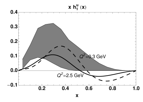
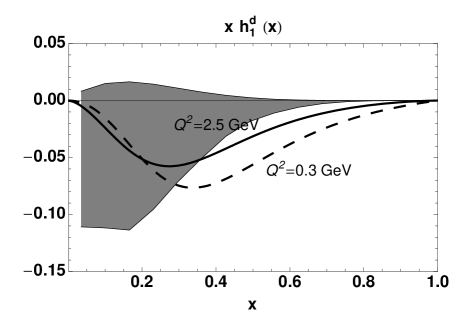
Refer to caption
Refer to caption
Figure 8: The transversity distribution xh1(x)𝑥subscript1𝑥xh_{1}(x) for up (left panel) and down quark (right panel). Dashed (solid) line for the model result before (after) the evolution at LO using the code of Ref. Hirai:1997mm up to the scale of the parametrization from Ref. Anselmino:2007fs , whose uncertainty band due to errors in the fit parameter is represented by the shaded area.

III.4 Transversity

In Fig. 8, the predictions of the spectator diquark model for the transversity distribution are compared with the only available parametrization of Ref. Anselmino:2007fs . In the left panel, xh1u(x)𝑥superscriptsubscript1𝑢𝑥xh_{1}^{u}(x) is shown, whereas xh1d(x)𝑥superscriptsubscript1𝑑𝑥xh_{1}^{d}(x) is shown in the right panel. All the model results at the assumed original scale Q02=0.3superscriptsubscript𝑄020.3Q_{0}^{2}=0.3 GeV2 are represented by the dashed line. The solid line indicates the result after applying the DGLAP evolution at LO up to the scale Q2=2.5superscript𝑄22.5Q^{2}=2.5 GeV2 using the code from Ref. Hirai:1997mm . The latter scale pertains the parametrization of Ref. Anselmino:2007fs , whose errors in the fit parameters produce the uncertainty band represented by the shaded area. The model is in reasonable agreement with the parametrization, with the maxima in the correct position and a somewhat too small result for the up quark at small x𝑥x. It should also be kept in mind that the present data reach at most x0.4𝑥0.4x\approx 0.4 Airapetian:2004tw ; Ageev:2006da and, moreover, the ansatz of Ref. Anselmino:2007fs does not allow for a sign change.444We point out that new fits of the transversity distribution functions have been presented at some conferences Anselmino:2008sj but not published yet.

Interestingly, for the up quark the model predicts a change of sign at x0.5similar-to𝑥0.5x\sim 0.5. To our knowledge, no other model of transversity displays this feature (see Ref. Barone:2001sp and references therein; see also recent calculations in Refs. Pasquini:2005dk ; Wakamatsu:2007nc ; Cloet:2007em ). The reason for this sign change is that the contribution of the vector diquark is negative, as evident from Eq.(79). In our model, at moderate x𝑥x the scalar diquark contribution is dominant, whereas at sufficiently high x𝑥x the contribution of the vector diquark becomes in absolute size bigger, thus leading to the sign change. Other versions of the diquark model, even with vector diquarks, may not show this property. This is already evident from inspecting the results (listed in the appendices) for different choices of the diquark polarization sum. We don’t think that our model calculation should be trusted more than others. Nevertheless, it might be interesting to contemplate the possibility of a sign change when choosing a form for the parametrization of the transversity function in “global fits.”
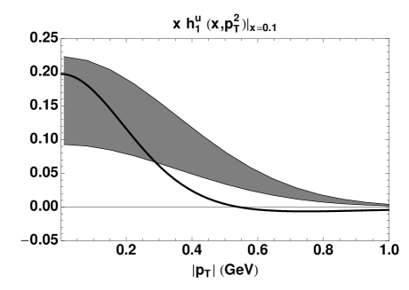
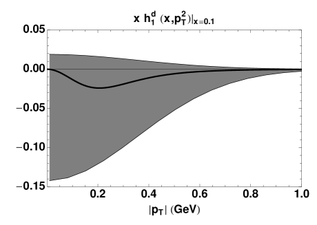
Refer to caption
Refer to caption
Figure 9: Same as in the previous figure, but for the 𝒑Tsubscript𝒑𝑇{\bm{p}}_{\scriptscriptstyle T} dependence of transversity at x=0.1𝑥0.1x=0.1.

In Fig. 9, the same comparison is performed as in the previous figure, but for the 𝒑Tsubscript𝒑𝑇{\bm{p}}_{\scriptscriptstyle T} dependence of the transversity at x=0.1𝑥0.1x=0.1, as it is deduced from Eqs. (68,69). Again, there is a reasonable agreement between model predictions and parametrizations but for the trend of the result for the up quark at |𝒑T|>0.3subscript𝒑𝑇0.3|{\bm{p}}_{\scriptscriptstyle T}|>0.3 GeV/c𝑐c. However, we stress that the comparison may be affected by the different scale of the model results (Q2=0.3superscript𝑄20.3Q^{2}=0.3 GeV2) and the one at which the parametrizations are extracted (Q2=2.5superscript𝑄22.5Q^{2}=2.5 GeV2). The proper evolution of the TMDs has not been considered yet. It is interesting to point out that in our model h1u(x,𝒑T2)superscriptsubscript1𝑢𝑥superscriptsubscript𝒑𝑇2h_{1}^{u}(x,{\bm{p}}_{\scriptscriptstyle T}^{2}) changes sign at 𝒑T0.5similar-tosubscript𝒑𝑇0.5{\bm{p}}_{\scriptscriptstyle T}\sim 0.5 GeV. This is due to the fact that the vector diquark contribution is always negative and dominant at high 𝒑Tsubscript𝒑𝑇{\bm{p}}_{\scriptscriptstyle T}. For the down quark, we note that h1d(x,0)=0superscriptsubscript1𝑑𝑥00h_{1}^{d}(x,0)=0, because the vector-diquark contribution to h1subscript1h_{1} is entirely given by LCWFs with nonvanishing orbital angular momentum.
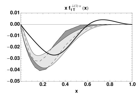
Refer to caption
Refer to caption
Figure 10: The first 𝒑Tsubscript𝒑𝑇{\bm{p}}_{\scriptscriptstyle T}-moment xf1T(1)(x)𝑥superscriptsubscript𝑓1𝑇perpendicular-toabsent1𝑥xf_{1T}^{\perp\,(1)}(x) of the Sivers function; left (right) panel for up (down) quark. Solid line for the results of the spectator diquark model. Darker shaded area for the uncertainty band due to the statistical error of the quark parametrizations from Ref. Anselmino:2008sg , lighter one from Ref. Collins:2005wb .

III.5 Sivers function

In Fig. 10, the xf1T(1)(x)𝑥superscriptsubscript𝑓1𝑇perpendicular-toabsent1𝑥xf_{1T}^{\perp\,(1)}(x) moment of the Sivers function, predicted using Eqs. (104) and (105), is given by the solid line and it is compared with two different parametrizations of the same observable. The darker shaded area represents the uncertainty due to the statistical errors in the parametrization of Ref. Anselmino:2008sg , while the lighter shaded area corresponds to the same for Ref. Collins:2005wb . Left panel refers to the up quark, right panel to down quark. First of all, we observe the agreement between the signs of the various flavor components, which also agree with the findings from calculations on the lattice Gockeler:2006zu . Also the maxima are reached at approximately the same x0.3similar-to𝑥0.3x\sim 0.3 as the parametrizations. Instead, the “strength” of the asymmetry (related to the modulus of each moment) is too much weaker for the down quark, while it seems reasonable for the up one. Again, it must be stressed that no evolution was applied in the displayed model results.
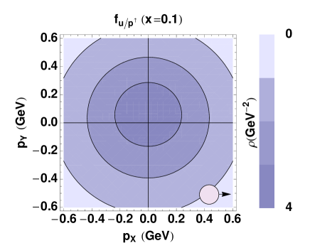
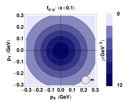
Refer to caption
Refer to caption
Figure 11: The model result for the spin density of unpolarized quarks in transversely polarized protons (see text for the precise definition) in 𝒑Tsubscript𝒑𝑇\bm{p}_{\scriptscriptstyle T} space at x=0.1𝑥0.1x=0.1. Left panel for up quark, right panel for down quark. The circle with the arrow indicates the direction of the proton polarization.

According to the Trento conventions Bacchetta:2004jz , we define the spin density of unpolarized quarks with flavor q𝑞q in transversely polarized protons as

fq/p(x,𝒑T)=f1q(x,𝒑T2)f1Tq(x,𝒑T2)(𝑷^×𝒑T)𝑺M.subscript𝑓𝑞superscript𝑝𝑥subscript𝒑𝑇superscriptsubscript𝑓1𝑞𝑥superscriptsubscript𝒑𝑇2superscriptsubscript𝑓1𝑇perpendicular-toabsent𝑞𝑥superscriptsubscript𝒑𝑇2^𝑷subscript𝒑𝑇𝑺𝑀f_{q/p^{\uparrow}}(x,\bm{p}_{\scriptscriptstyle T})=f_{1}^{q}(x,\bm{p}_{\scriptscriptstyle T}^{2})-f_{1T}^{\perp\,q}(x,\bm{p}_{\scriptscriptstyle T}^{2})\,\frac{(\hat{\bm{P}}\times\bm{p}_{\scriptscriptstyle T})\,\cdot\,\bm{S}}{M}\;. (130)

In a SIDIS experiment, typically 𝑷^^𝑷\hat{\bm{P}} is antialigned to the 𝒛^^𝒛\hat{\bm{z}} axis that points in the direction of the momentum transfer 𝒒𝒒\bm{q}. Hence, if the proton polarization is chosen along the 𝒙^^𝒙\hat{\bm{x}} axis, the spin density (130) shows an asymmetry in momentum space along the pysubscript𝑝𝑦p_{y} direction, whose size is driven by the Sivers function. In Fig. 11, we show fq/p(0.1,𝒑T)subscript𝑓𝑞superscript𝑝0.1subscript𝒑𝑇f_{q/p^{\uparrow}}(0.1,\bm{p}_{\scriptscriptstyle T}) for q=u𝑞𝑢q=u (left panel) and q=d𝑞𝑑q=d (right panel). Since the Sivers function for the up (down) quark is negative (positive), the density is deformed towards positive (negative) values of pysubscript𝑝𝑦p_{y}. This feature is in agreement with the lattice results of Ref. Gockeler:2006zu and with the signs of the anomalous magnetic moments κqsuperscript𝜅𝑞\kappa^{q} Burkardt:2002ks .

III.6 Boer-Mulders function

Refer to caption
Refer to caption
Figure 12: The xh1(1)(x)𝑥superscriptsubscript1perpendicular-toabsent1𝑥xh_{1}^{\perp\,(1)}(x) (left) and xh1(1/2)(x)𝑥superscriptsubscript1perpendicular-toabsent12𝑥xh_{1}^{\perp\,(1/2)}(x) (right) moments of the Boer-Mulders function. Solid and dashed lines for up and down quarks, respectively.

In Fig. 12, the xh1(1)(x)𝑥superscriptsubscript1perpendicular-toabsent1𝑥xh_{1}^{\perp\,(1)}(x) and xh1(1/2)(x)𝑥superscriptsubscript1perpendicular-toabsent12𝑥xh_{1}^{\perp\,(1/2)}(x) moments of the Boer-Mulders function, as deduced from Eqs. (106,107) and (110,111), are displayed in the left and right panel, respectively. The solid lines correspond to the results for the up quark; dashed lines for the down quark. For the Boer-Mulders function, the only available parametrization appeared recently in Zhang:2008nu , but the overall normalization depends on a parameter ω𝜔\omega that cannot be fixed with available experimental information. Our result agrees in sign and shape with that extraction. The absolute values of our functions correspond to ω0.3𝜔0.3\omega\approx 0.3. We remark that there is full agreement between the sign of the u𝑢u and d𝑑d components and the aforementioned lattice calculations Gockeler:2006zu , as observed also in a different version of the spectator model Gamberg:2007wm and in the bag model Yuan:2003wk . This agreement seems to be a general feature, as argued in Ref. Burkardt:2007xm 555A different result for the sign of the down quark Boer-Mulders function was obtained in Ref. Bacchetta:2003rz , probably due to a mistake in that calculation (see App. B.4).

In Fig. 13, we show, again at x=0.1𝑥0.1x=0.1, the spin density of transversely polarized quarks with flavor q𝑞q in unpolarized protons, related to the Boer-Mulders effect by Bacchetta:2004jz

fq/p(x,𝒑T)=12[f1q(x,𝒑T2)h1q(x,𝒑T2)(𝑷^×𝒑T)𝑺qM],subscript𝑓superscript𝑞𝑝𝑥subscript𝒑𝑇12delimited-[]superscriptsubscript𝑓1𝑞𝑥superscriptsubscript𝒑𝑇2superscriptsubscript1perpendicular-toabsent𝑞𝑥superscriptsubscript𝒑𝑇2^𝑷subscript𝒑𝑇subscript𝑺𝑞𝑀f_{q^{\uparrow}/p}(x,\bm{p}_{\scriptscriptstyle T})=\frac{1}{2}\,\left[f_{1}^{q}(x,\bm{p}_{\scriptscriptstyle T}^{2})-h_{1}^{\perp\,q}(x,\bm{p}_{\scriptscriptstyle T}^{2})\,\frac{(\hat{\bm{P}}\times\bm{p}_{\scriptscriptstyle T})\,\cdot\,\bm{S}_{q}}{M}\right]\;, (131)

where now the quark polarization 𝑺qsubscript𝑺𝑞\bm{S}_{q} points along 𝒙^^𝒙\hat{\bm{x}}. Since the Boer-Mulders function is negative for both flavors (see Fig. 12), the related spin density is always deformed towards positive pysubscript𝑝𝑦p_{y}, again in agreement with the lattice results Gockeler:2006zu .
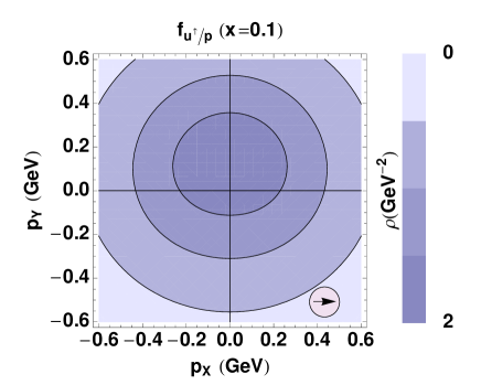
Refer to caption
Refer to caption
Figure 13: The model result for the spin density of transversely polarized quarks in unpolarized protons (see text for the precise definition) in 𝒑Tsubscript𝒑𝑇\bm{p}_{\scriptscriptstyle T} space at x=0.1𝑥0.1x=0.1. Left panel for up quark, right panel for down quark. The arrow inside the circle indicates the direction of the quark polarization.

IV Conclusions

We have presented a systematic calculation of all leading-twist parton distributions in the nucleon in a diquark spectator model. We have generated the relative phase necessary to produce T-odd structures by approximating the gauge link operator with a one gluon-exchange interaction. All results have been presented in analytic form and interpreted in terms of overlaps of light-cone wavefunctions.

We tried to extend and improve the spectator model calculations presented in Refs. Jakob:1997wg ; Bacchetta:2003rz ; Gamberg:2007wm by considering several choices of the axial-vector diquark polarization states and of the nucleon-quark-diquark form factor. We listed the analytic expressions for all possible choices in the appendices. We critically reconsidered some of the limits of the model and the choice of model parameters used in the past literature. In particular, we showed that the spectator diquark model is not able to reproduce both the quark number and momentum sum rule at the same time, because the diquark is considered as a charged parton, hence active in the sum rules. We argued that the proton wave function does not show the usual SU(4)=SU(2)tensor-product\otimesSU(2) symmetry Jakob:1997wg , since the quark-diquark system in its ground state can have a nonvanishing relative orbital angular momentum.

For numerical studies, we chose the version of the model that in our opinion is more sensible and practical, i.e., the one where only light-cone transverse polarizations of the diquark are present and a dipolar form factor is used. We identified nine free parameters of the model and we fixed them by reproducing the phenomenological parametrization of unpolarized Chekanov:2002pv and longitudinally polarized Gluck:2000dy parton distributions at the lowest available scale, i.e. Q2=0.3superscript𝑄20.3Q^{2}=0.3 and 0.260.260.26 GeV2, respectively.

Whenever possible, results have been compared with available parametrizations. For the chiral-odd transversity distribution, there is only one available from Ref. Anselmino:2007fs , which was deduced from SSA data at Q2=2.5superscript𝑄22.5Q^{2}=2.5 GeV2. The 𝒑Tsubscript𝒑𝑇\bm{p}_{\scriptscriptstyle T}-integrated model result, once evolved to this scale using the code from Ref. Hirai:1997mm at LO, displays a satisfactory overall agreement. The f1T(1)(x)superscriptsubscript𝑓1𝑇perpendicular-toabsent1𝑥f_{1T}^{\perp\,(1)}(x) moment of the chiral-even T-odd Sivers function f1Tsuperscriptsubscript𝑓1𝑇perpendicular-tof_{1T}^{\perp} was compared with the parametrizations of Refs. Anselmino:2008sg ; Collins:2005wb . There is agreement between the signs of the various flavor components and between the positions of the maxima in x𝑥x, but the absolute value of the function is somewhat too small for the down quark. The comparison is affected by the difference of the scales, since evolution equations for the Sivers function have not been used. We also plotted the h1(1)(x)superscriptsubscript1perpendicular-toabsent1𝑥h_{1}^{\perp\,(1)}(x) and h1(1/2)(x)superscriptsubscript1perpendicular-toabsent12𝑥h_{1}^{\perp\,(1/2)}(x) moments of the chiral-odd T-odd Boer-Mulders function h1superscriptsubscript1perpendicular-toh_{1}^{\perp}. We have also shown the quark spin densities defined in the Trento conventions Bacchetta:2004jz , as produced in turn by the Sivers or the Boer-Mulders effects. For unpolarized quarks in transversely polarized protons, the spin density fq/psubscript𝑓𝑞superscript𝑝f_{q/p^{\uparrow}} is linked to f1Tsuperscriptsubscript𝑓1𝑇perpendicular-tof_{1T}^{\perp}, while for transversely polarized quarks in unpolarized protons the fq/psubscript𝑓superscript𝑞𝑝f_{q^{\uparrow}/p} is linked to h1superscriptsubscript1perpendicular-toh_{1}^{\perp}. For transverse polarizations along the 𝒙^^𝒙\hat{\bm{x}} axis, the contour plot in the quark momentum space of such densities at x=0.1𝑥0.1x=0.1 displays a distortion in the pysubscript𝑝𝑦p_{y} direction, whose sign is consistent with the lattice findings for the corresponding spin densities in impact parameter space Gockeler:2006zu .

Using the model parton densities discussed above, various spin, beam, and azimuthal asymmetries in semi-inclusive hadronic reactions can be predicted, which are of interest for several experimental collaborations. Model calculations can be useful to interpret experimental measurements, helping us to explore spin-orbit parton correlations inside hadrons and shed light on the well-known puzzle of the proton spin sum rule.

Acknowledgments

F. C. and M. R. would like to thank B. Pasquini for useful discussions.

This work is part of the European Integrated Infrastructure Initiative in Hadronic Physics project under Contract No. RII3-CT-2004-506078.

Authored by Jefferson Science Associates, LLC under U.S. DOE Contract No. DE-AC05-06OR23177. The U.S. Government retains a non-exclusive, paid-up, irrevocable, world-wide license to publish or reproduce this manuscript for U.S. Government purposes.

Appendix A T-even functions in different variations of the model

In this Appendix we list the leading-twist T-even parton densities obtained in the context of our spectator diquark model, for all the choices of axial-vector diquark polarization sum and nucleon-quark-diquark vertex. To avoid overloading the notation, we will use the same ones for the parameters involved (gXsubscript𝑔𝑋g_{X}, MXsubscript𝑀𝑋M_{X}, ΛXsubscriptΛ𝑋\Lambda_{X}). However, it must be kept in mind that the numerical value of these parameters can be different in the various versions of the model.

A.1 Scalar diquark

The results for the scalar diquark are

f1q(s)(x,𝒑T2)superscriptsubscript𝑓1𝑞𝑠𝑥superscriptsubscript𝒑𝑇2\displaystyle f_{1}^{q(s)}(x,{\bm{p}}_{\scriptscriptstyle T}^{2}) =gs2(2π)3[(m+xM)2+𝒑T2](1x)2[𝒑T2+Ls2(m2)]2absentsuperscriptsubscript𝑔𝑠2superscript2𝜋3delimited-[]superscript𝑚𝑥𝑀2superscriptsubscript𝒑𝑇21𝑥2superscriptdelimited-[]superscriptsubscript𝒑𝑇2superscriptsubscript𝐿𝑠2superscript𝑚22\displaystyle=\frac{g_{s}^{2}}{(2\pi)^{3}}\,\frac{[(m+xM)^{2}+{\bm{p}}_{\scriptscriptstyle T}^{2}]\,(1-x)}{2\,[{\bm{p}}_{\scriptscriptstyle T}^{2}+L_{s}^{2}(m^{2})]^{2}} (132)
g1Lq(s)(x,𝒑T2)superscriptsubscript𝑔1𝐿𝑞𝑠𝑥superscriptsubscript𝒑𝑇2\displaystyle g_{1L}^{q(s)}(x,{\bm{p}}_{\scriptscriptstyle T}^{2}) =gs2(2π)3[(m+xM)2𝒑T2](1x)2[𝒑T2+Ls2(m2)]2,absentsuperscriptsubscript𝑔𝑠2superscript2𝜋3delimited-[]superscript𝑚𝑥𝑀2superscriptsubscript𝒑𝑇21𝑥2superscriptdelimited-[]superscriptsubscript𝒑𝑇2superscriptsubscript𝐿𝑠2superscript𝑚22\displaystyle=\frac{g_{s}^{2}}{(2\pi)^{3}}\,\frac{[(m+xM)^{2}-{\bm{p}}_{\scriptscriptstyle T}^{2}]\,(1-x)}{2\,[{\bm{p}}_{\scriptscriptstyle T}^{2}+L_{s}^{2}(m^{2})]^{2}}\;, (133)
g1Tq(s)(x,𝒑T2)superscriptsubscript𝑔1𝑇𝑞𝑠𝑥superscriptsubscript𝒑𝑇2\displaystyle g_{1T}^{q(s)}(x,{\bm{p}}_{\scriptscriptstyle T}^{2}) =gs2(2π)3M(m+xM)(1x)[𝒑T2+Ls2(m2)]2,absentsuperscriptsubscript𝑔𝑠2superscript2𝜋3𝑀𝑚𝑥𝑀1𝑥superscriptdelimited-[]superscriptsubscript𝒑𝑇2superscriptsubscript𝐿𝑠2superscript𝑚22\displaystyle=\frac{g_{s}^{2}}{(2\pi)^{3}}\,\frac{M\,(m+xM)\,(1-x)}{[{\bm{p}}_{\scriptscriptstyle T}^{2}+L_{s}^{2}(m^{2})]^{2}}\;, (134)
h1Lq(s)(x,𝒑T2)superscriptsubscript1𝐿perpendicular-toabsent𝑞𝑠𝑥superscriptsubscript𝒑𝑇2\displaystyle h_{1L}^{\perp\,q(s)}(x,{\bm{p}}_{\scriptscriptstyle T}^{2}) =g1Tq(s)(x,𝒑T2),absentsuperscriptsubscript𝑔1𝑇𝑞𝑠𝑥superscriptsubscript𝒑𝑇2\displaystyle=-g_{1T}^{q(s)}(x,{\bm{p}}_{\scriptscriptstyle T}^{2})\;, (135)
h1Tq(s)(x,𝒑T2)superscriptsubscript1𝑇𝑞𝑠𝑥superscriptsubscript𝒑𝑇2\displaystyle h_{1T}^{q(s)}(x,{\bm{p}}_{\scriptscriptstyle T}^{2}) =f1q(s)(x,𝒑T2),absentsuperscriptsubscript𝑓1𝑞𝑠𝑥superscriptsubscript𝒑𝑇2\displaystyle=f_{1}^{q(s)}(x,{\bm{p}}_{\scriptscriptstyle T}^{2})\;, (136)
h1Tq(s)(x,𝒑T2)superscriptsubscript1𝑇perpendicular-toabsent𝑞𝑠𝑥superscriptsubscript𝒑𝑇2\displaystyle h_{1T}^{\perp\,q(s)}(x,{\bm{p}}_{\scriptscriptstyle T}^{2}) =gs2(2π)3M2(1x)[𝒑T2+Ls2(m2)]2,absentsuperscriptsubscript𝑔𝑠2superscript2𝜋3superscript𝑀21𝑥superscriptdelimited-[]superscriptsubscript𝒑𝑇2superscriptsubscript𝐿𝑠2superscript𝑚22\displaystyle=-\frac{g_{s}^{2}}{(2\pi)^{3}}\,\frac{M^{2}\,(1-x)}{[{\bm{p}}_{\scriptscriptstyle T}^{2}+L_{s}^{2}(m^{2})]^{2}}\;, (137)

where we recall that M𝑀M is the nucleon mass and m𝑚m is the mass of the parton. From the latter two densities, we construct the contribution of the scalar diquark to the transversity:

h1q(s)(x,𝒑T2)=h1Tq(s)(x,𝒑T2)+𝒑T22M2h1Tq(s)(x,𝒑T2)=gs2(2π)3(m+xM)2(1x)2[𝒑T2+Ls2(m2)]2=12(f1q(s)(x,𝒑T2)+g1q(s)(x,𝒑T2)).superscriptsubscript1𝑞𝑠𝑥superscriptsubscript𝒑𝑇2superscriptsubscript1𝑇𝑞𝑠𝑥superscriptsubscript𝒑𝑇2superscriptsubscript𝒑𝑇22superscript𝑀2superscriptsubscript1𝑇perpendicular-toabsent𝑞𝑠𝑥superscriptsubscript𝒑𝑇2superscriptsubscript𝑔𝑠2superscript2𝜋3superscript𝑚𝑥𝑀21𝑥2superscriptdelimited-[]superscriptsubscript𝒑𝑇2superscriptsubscript𝐿𝑠2superscript𝑚2212superscriptsubscript𝑓1𝑞𝑠𝑥superscriptsubscript𝒑𝑇2superscriptsubscript𝑔1𝑞𝑠𝑥superscriptsubscript𝒑𝑇2\begin{split}h_{1}^{q(s)}(x,{\bm{p}}_{\scriptscriptstyle T}^{2})&=h_{1T}^{q(s)}(x,{\bm{p}}_{\scriptscriptstyle T}^{2})+\frac{{\bm{p}}_{\scriptscriptstyle T}^{2}}{2M^{2}}\,h_{1T}^{\perp\,q(s)}(x,{\bm{p}}_{\scriptscriptstyle T}^{2})\\ &=\frac{g_{s}^{2}}{(2\pi)^{3}}\,\frac{(m+xM)^{2}\,(1-x)}{2\,[{\bm{p}}_{\scriptscriptstyle T}^{2}+L_{s}^{2}(m^{2})]^{2}}=\frac{1}{2}\,\left(f_{1}^{q(s)}(x,{\bm{p}}_{\scriptscriptstyle T}^{2})+g_{1}^{q(s)}(x,{\bm{p}}_{\scriptscriptstyle T}^{2})\right)\;.\end{split} (138)

The above results are valid for a point-like nucleon-quark-diquark coupling. For the other form factors it is sufficient to apply the replacements

gs2superscriptsubscript𝑔𝑠2\displaystyle g_{s}^{2} gs2(1x)2[𝒑T2+Ls2(m2)]2[𝒑T2+Ls2(Λs2)]4absentsuperscriptsubscript𝑔𝑠2superscript1𝑥2superscriptdelimited-[]superscriptsubscript𝒑𝑇2superscriptsubscript𝐿𝑠2superscript𝑚22superscriptdelimited-[]superscriptsubscript𝒑𝑇2superscriptsubscript𝐿𝑠2superscriptsubscriptΛ𝑠24\displaystyle\to g_{s}^{2}(1-x)^{2}\frac{[{\bm{p}}_{\scriptscriptstyle T}^{2}+L_{s}^{2}(m^{2})]^{2}}{[{\bm{p}}_{\scriptscriptstyle T}^{2}+L_{s}^{2}(\Lambda_{s}^{2})]^{4}} dipolar form factor, (139)
gs2superscriptsubscript𝑔𝑠2\displaystyle g_{s}^{2} gs2e[𝒑T2+LX2(m2)]/[(1x)ΛX2]absentsuperscriptsubscript𝑔𝑠2superscript𝑒delimited-[]superscriptsubscript𝒑𝑇2superscriptsubscript𝐿𝑋2superscript𝑚2delimited-[]1𝑥superscriptsubscriptΛ𝑋2\displaystyle\to g_{s}^{2}e^{\,-[{\bm{p}}_{\scriptscriptstyle T}^{2}+L_{X}^{2}(m^{2})]/[(1-x)\,\Lambda_{X}^{2}]} exponential form factor. (140)

The integrated results are obviously different for the three form-factor choices. In all cases the transversity function saturates the Soffer bound, i.e.,

h1q(s)(x)=12(f1q(s)(x)+g1q(s)(x)).superscriptsubscript1𝑞𝑠𝑥12superscriptsubscript𝑓1𝑞𝑠𝑥superscriptsubscript𝑔1𝑞𝑠𝑥h_{1}^{q(s)}(x)=\frac{1}{2}\,\left(f_{1}^{q(s)}(x)+g_{1}^{q(s)}(x)\right). (141)
  • Point-like coupling (to avoid divergences we assume that the 𝒑T2superscriptsubscript𝒑𝑇2\bm{p}_{\scriptscriptstyle T}^{2} integration is extended up to a finite cutoff Λs2superscriptsubscriptΛ𝑠2\Lambda_{s}^{2})

    f1q(s)(x)superscriptsubscript𝑓1𝑞𝑠𝑥\displaystyle f_{1}^{q(s)}(x) =gs2(1x)(2π)2(m+xM)2Λs2Ls2(m2)Λs2+Ls2(m2)[Λs2+Ls2(m2)]log(Λs2Ls2(m2)+1)4Ls2(m2)[Λs2+Ls2(m2)],absentsuperscriptsubscript𝑔𝑠21𝑥superscript2𝜋2superscript𝑚𝑥𝑀2superscriptsubscriptΛ𝑠2superscriptsubscript𝐿𝑠2superscript𝑚2superscriptsubscriptΛ𝑠2superscriptsubscript𝐿𝑠2superscript𝑚2delimited-[]superscriptsubscriptΛ𝑠2superscriptsubscript𝐿𝑠2superscript𝑚2superscriptsubscriptΛ𝑠2superscriptsubscript𝐿𝑠2superscript𝑚214superscriptsubscript𝐿𝑠2superscript𝑚2delimited-[]superscriptsubscriptΛ𝑠2superscriptsubscript𝐿𝑠2superscript𝑚2\displaystyle=\frac{g_{s}^{2}\,(1-x)}{(2\pi)^{2}}\,\frac{(m+xM)^{2}\,\Lambda_{s}^{2}-L_{s}^{2}(m^{2})\,\Lambda_{s}^{2}+L_{s}^{2}(m^{2})\,[\Lambda_{s}^{2}+L_{s}^{2}(m^{2})]\,\log\left(\frac{\Lambda_{s}^{2}}{L_{s}^{2}(m^{2})}+1\right)}{4\,L_{s}^{2}(m^{2})\,[\Lambda_{s}^{2}+L_{s}^{2}(m^{2})]}\;, (142)
    g1q(s)(x)superscriptsubscript𝑔1𝑞𝑠𝑥\displaystyle g_{1}^{q(s)}(x) =gs2(1x)(2π)2(m+xM)2Λs2+Ls2(m2)Λs2Ls2(m2)[Λs2+Ls2(m2)]log(Λs2Ls2(m2)+1)4Ls2(m2)[Λs2+Ls2(m2)],absentsuperscriptsubscript𝑔𝑠21𝑥superscript2𝜋2superscript𝑚𝑥𝑀2superscriptsubscriptΛ𝑠2superscriptsubscript𝐿𝑠2superscript𝑚2superscriptsubscriptΛ𝑠2superscriptsubscript𝐿𝑠2superscript𝑚2delimited-[]superscriptsubscriptΛ𝑠2superscriptsubscript𝐿𝑠2superscript𝑚2superscriptsubscriptΛ𝑠2superscriptsubscript𝐿𝑠2superscript𝑚214superscriptsubscript𝐿𝑠2superscript𝑚2delimited-[]superscriptsubscriptΛ𝑠2superscriptsubscript𝐿𝑠2superscript𝑚2\displaystyle=\frac{g_{s}^{2}\,(1-x)}{(2\pi)^{2}}\,\frac{(m+xM)^{2}\,\Lambda_{s}^{2}+L_{s}^{2}(m^{2})\,\Lambda_{s}^{2}-L_{s}^{2}(m^{2})\,[\Lambda_{s}^{2}+L_{s}^{2}(m^{2})]\,\log\left(\frac{\Lambda_{s}^{2}}{L_{s}^{2}(m^{2})}+1\right)}{4\,L_{s}^{2}(m^{2})\,[\Lambda_{s}^{2}+L_{s}^{2}(m^{2})]}\;, (143)
  • Dipolar form factor [same as Eqs. (74) and (76)]

    f1q(s)(x)superscriptsubscript𝑓1𝑞𝑠𝑥\displaystyle f_{1}^{q(s)}(x) =gs2(2π)2[2(m+xM)2+Ls2(Λs2)](1x)324Ls6(Λs2)absentsuperscriptsubscript𝑔𝑠2superscript2𝜋2delimited-[]2superscript𝑚𝑥𝑀2superscriptsubscript𝐿𝑠2superscriptsubscriptΛ𝑠2superscript1𝑥324superscriptsubscript𝐿𝑠6superscriptsubscriptΛ𝑠2\displaystyle=\frac{g_{s}^{2}}{(2\pi)^{2}}\,\frac{[2\,(m+xM)^{2}+L_{s}^{2}(\Lambda_{s}^{2})]\,(1-x)^{3}}{24\,L_{s}^{6}(\Lambda_{s}^{2})} (144)
    g1q(s)(x)superscriptsubscript𝑔1𝑞𝑠𝑥\displaystyle g_{1}^{q(s)}(x) =gs2(2π)2[2(m+xM)2Ls2(Λs2)](1x)324Ls6(Λs2)absentsuperscriptsubscript𝑔𝑠2superscript2𝜋2delimited-[]2superscript𝑚𝑥𝑀2superscriptsubscript𝐿𝑠2superscriptsubscriptΛ𝑠2superscript1𝑥324superscriptsubscript𝐿𝑠6superscriptsubscriptΛ𝑠2\displaystyle=\frac{g_{s}^{2}}{(2\pi)^{2}}\,\frac{[2\,(m+xM)^{2}-L_{s}^{2}(\Lambda_{s}^{2})]\,(1-x)^{3}}{24\,L_{s}^{6}(\Lambda_{s}^{2})} (145)
  • Exponential form factor

    f1q(s)(x)=gs2(2π)214{e2Ls2(m2)/[(1x)Λs2]1xLs2(m2)[(m+xM)2Ls2(m2)]Γ(0,2Ls2(m2)(1x)Λs2)2[(m+xM)2Ls2(m2)](1x)Λs2Λs2},superscriptsubscript𝑓1𝑞𝑠𝑥superscriptsubscript𝑔𝑠2superscript2𝜋214superscript𝑒2superscriptsubscript𝐿𝑠2superscript𝑚2delimited-[]1𝑥superscriptsubscriptΛ𝑠21𝑥superscriptsubscript𝐿𝑠2superscript𝑚2delimited-[]superscript𝑚𝑥𝑀2superscriptsubscript𝐿𝑠2superscript𝑚2Γ02superscriptsubscript𝐿𝑠2superscript𝑚21𝑥superscriptsubscriptΛ𝑠22delimited-[]superscript𝑚𝑥𝑀2superscriptsubscript𝐿𝑠2superscript𝑚21𝑥superscriptsubscriptΛ𝑠2superscriptsubscriptΛ𝑠2\displaystyle\begin{split}f_{1}^{q(s)}(x)&=\frac{g_{s}^{2}}{(2\pi)^{2}}\,\frac{1}{4}\,\Bigg{\{}e^{\,-2\,L_{s}^{2}(m^{2})/[(1-x)\,\Lambda_{s}^{2}]}\,\frac{1-x}{L_{s}^{2}(m^{2})}\,\bigl{[}(m+xM)^{2}-L_{s}^{2}(m^{2})\bigr{]}\\ &\hskip 85.35826pt-\Gamma\left(0,\frac{2L_{s}^{2}(m^{2})}{(1-x)\,\Lambda_{s}^{2}}\right)\,\frac{2\,\bigl{[}(m+xM)^{2}-L_{s}^{2}(m^{2})\bigr{]}-(1-x)\,\Lambda_{s}^{2}}{\Lambda_{s}^{2}}\Bigg{\}}\;,\end{split} (146)
    g1q(s)(x)=gs2(2π)214{e2Ls2(m2)/[(1x)Λs2]1xLs2(m2)[(m+xM)2+Ls2(m2)]Γ(0,2Ls2(m2)(1x)Λs2)2[(m+xM)2+Ls2(m2)]+Λs2(1x)Λs2},superscriptsubscript𝑔1𝑞𝑠𝑥superscriptsubscript𝑔𝑠2superscript2𝜋214superscript𝑒2superscriptsubscript𝐿𝑠2superscript𝑚2delimited-[]1𝑥superscriptsubscriptΛ𝑠21𝑥superscriptsubscript𝐿𝑠2superscript𝑚2delimited-[]superscript𝑚𝑥𝑀2superscriptsubscript𝐿𝑠2superscript𝑚2Γ02superscriptsubscript𝐿𝑠2superscript𝑚21𝑥superscriptsubscriptΛ𝑠22delimited-[]superscript𝑚𝑥𝑀2superscriptsubscript𝐿𝑠2superscript𝑚2superscriptsubscriptΛ𝑠21𝑥superscriptsubscriptΛ𝑠2\displaystyle\begin{split}g_{1}^{q(s)}(x)&=\frac{g_{s}^{2}}{(2\pi)^{2}}\,\frac{1}{4}\,\Bigg{\{}e^{\,-2\,L_{s}^{2}(m^{2})/[(1-x)\,\Lambda_{s}^{2}]}\,\frac{1-x}{L_{s}^{2}(m^{2})}\,\bigl{[}(m+xM)^{2}+L_{s}^{2}(m^{2})\bigr{]}\\ &\hskip 56.9055pt-\Gamma\left(0,\frac{2\,L_{s}^{2}(m^{2})}{(1-x)\,\Lambda_{s}^{2}}\right)\,\frac{2\,[(m+xM)^{2}+L_{s}^{2}(m^{2})]+\Lambda_{s}^{2}\,(1-x)}{\Lambda_{s}^{2}}\Bigg{\}}\;,\end{split} (147)

    where ΓΓ\Gamma is the incomplete ΓΓ\Gamma function, defined as

    Γ(a,z)=zta1et𝑑t.Γ𝑎𝑧superscriptsubscript𝑧superscript𝑡𝑎1superscript𝑒𝑡differential-d𝑡\Gamma(a,z)=\int_{z}^{\infty}t^{a-1}\,e^{-t}dt\;. (148)

A.2 Axial-vector diquark with light-cone transverse polarization only

The unintegrated parton densities are

f1q(a)(x,𝒑T2)superscriptsubscript𝑓1𝑞𝑎𝑥superscriptsubscript𝒑𝑇2\displaystyle f_{1}^{q(a)}(x,{\bm{p}}_{\scriptscriptstyle T}^{2}) =ga2(2π)3𝒑T2(1+x2)+(m+xM)2(1x)22[𝒑T2+La2(m2)]2(1x)absentsuperscriptsubscript𝑔𝑎2superscript2𝜋3superscriptsubscript𝒑𝑇21superscript𝑥2superscript𝑚𝑥𝑀2superscript1𝑥22superscriptdelimited-[]superscriptsubscript𝒑𝑇2superscriptsubscript𝐿𝑎2superscript𝑚221𝑥\displaystyle=\frac{g_{a}^{2}}{(2\pi)^{3}}\,\frac{{\bm{p}}_{\scriptscriptstyle T}^{2}\,(1+x^{2})+(m+xM)^{2}\,(1-x)^{2}}{2\,[{\bm{p}}_{\scriptscriptstyle T}^{2}+L_{a}^{2}(m^{2})]^{2}\,(1-x)}
g1Lq(a)(x,𝒑T2)superscriptsubscript𝑔1𝐿𝑞𝑎𝑥superscriptsubscript𝒑𝑇2\displaystyle g_{1L}^{q(a)}(x,{\bm{p}}_{\scriptscriptstyle T}^{2}) =ga2(2π)3𝒑T2(1+x2)(m+xM)2(1x)22[𝒑T2+La2(m2)]2(1x),absentsuperscriptsubscript𝑔𝑎2superscript2𝜋3superscriptsubscript𝒑𝑇21superscript𝑥2superscript𝑚𝑥𝑀2superscript1𝑥22superscriptdelimited-[]superscriptsubscript𝒑𝑇2superscriptsubscript𝐿𝑎2superscript𝑚221𝑥\displaystyle=\frac{g_{a}^{2}}{(2\pi)^{3}}\,\frac{{\bm{p}}_{\scriptscriptstyle T}^{2}\,(1+x^{2})-(m+xM)^{2}\,(1-x)^{2}}{2\,[{\bm{p}}_{\scriptscriptstyle T}^{2}+L_{a}^{2}(m^{2})]^{2}\,(1-x)}\;,
g1Tq(a)(x,𝒑T2)superscriptsubscript𝑔1𝑇𝑞𝑎𝑥superscriptsubscript𝒑𝑇2\displaystyle g_{1T}^{q(a)}(x,{\bm{p}}_{\scriptscriptstyle T}^{2}) =ga2(2π)3Mx(m+xM)[𝒑T2+La2(m2)]2,absentsuperscriptsubscript𝑔𝑎2superscript2𝜋3𝑀𝑥𝑚𝑥𝑀superscriptdelimited-[]superscriptsubscript𝒑𝑇2superscriptsubscript𝐿𝑎2superscript𝑚22\displaystyle=\frac{g_{a}^{2}}{(2\pi)^{3}}\,\frac{M\,x\,(m+xM)}{[{\bm{p}}_{\scriptscriptstyle T}^{2}+L_{a}^{2}(m^{2})]^{2}}\;,
h1Lq(a)(x,𝒑T2)superscriptsubscript1𝐿perpendicular-toabsent𝑞𝑎𝑥superscriptsubscript𝒑𝑇2\displaystyle h_{1L}^{\perp\,q(a)}(x,{\bm{p}}_{\scriptscriptstyle T}^{2}) =g1Tq(a)(x,𝒑T2)/x,absentsuperscriptsubscript𝑔1𝑇𝑞𝑎𝑥superscriptsubscript𝒑𝑇2𝑥\displaystyle=g_{1T}^{q(a)}(x,{\bm{p}}_{\scriptscriptstyle T}^{2})/x\;,
h1Tq(a)(x,𝒑T2)superscriptsubscript1𝑇𝑞𝑎𝑥superscriptsubscript𝒑𝑇2\displaystyle h_{1T}^{q(a)}(x,{\bm{p}}_{\scriptscriptstyle T}^{2}) =ga2(2π)3x𝒑T2[𝒑T2+La2(m2)]2(1x),absentsuperscriptsubscript𝑔𝑎2superscript2𝜋3𝑥superscriptsubscript𝒑𝑇2superscriptdelimited-[]superscriptsubscript𝒑𝑇2superscriptsubscript𝐿𝑎2superscript𝑚221𝑥\displaystyle=-\frac{g_{a}^{2}}{(2\pi)^{3}}\,\frac{x\,{\bm{p}}_{\scriptscriptstyle T}^{2}}{[{\bm{p}}_{\scriptscriptstyle T}^{2}+L_{a}^{2}(m^{2})]^{2}\,(1-x)}\;,
h1Tq(a)(x,𝒑T2)superscriptsubscript1𝑇perpendicular-toabsent𝑞𝑎𝑥superscriptsubscript𝒑𝑇2\displaystyle h_{1T}^{\perp\,q(a)}(x,{\bm{p}}_{\scriptscriptstyle T}^{2}) =0,absent0\displaystyle=0\;,
h1q(a)(x,𝒑T2)superscriptsubscript1𝑞𝑎𝑥superscriptsubscript𝒑𝑇2\displaystyle h_{1}^{q(a)}(x,{\bm{p}}_{\scriptscriptstyle T}^{2}) =h1Tq(a)(x,𝒑T2).absentsuperscriptsubscript1𝑇𝑞𝑎𝑥superscriptsubscript𝒑𝑇2\displaystyle=h_{1T}^{q(a)}(x,{\bm{p}}_{\scriptscriptstyle T}^{2})\;. (149)

The above results are valid for a point-like nucleon-quark-diquark coupling. For the other form factors it is sufficient to apply the replacements in Eqs. (139) and (140).

The integrated results are

  • Point-like coupling (to avoid divergences we assume that the 𝒑T2superscriptsubscript𝒑𝑇2\bm{p}_{\scriptscriptstyle T}^{2} integration is extended up to a finite cutoff Λa2superscriptsubscriptΛ𝑎2\Lambda_{a}^{2})

    f1q(a)(x)superscriptsubscript𝑓1𝑞𝑎𝑥\displaystyle f_{1}^{q(a)}(x) =ga2(2π)214La2(m2)[Λa2+La2(m2)](1x)[xΛa2[(M2m2)(1x2)+2mM(1x)2Ma2(1+x2)]\displaystyle=\frac{g_{a}^{2}}{(2\pi)^{2}}\,\frac{1}{4\,L_{a}^{2}(m^{2})\,[\Lambda_{a}^{2}+L_{a}^{2}(m^{2})]\,(1-x)}\,\Bigg{[}x\,\Lambda_{a}^{2}\,\left[(M^{2}-m^{2})\,(1-x^{2})+2mM\,(1-x)^{2}-M_{a}^{2}\,(1+x^{2})\right]
    +La2(m2)[Λa2+La2(m2)](1+x2)log(Λa2La2(m2)+1)],\displaystyle\quad+L_{a}^{2}(m^{2})\,[\Lambda_{a}^{2}+L_{a}^{2}(m^{2})]\,(1+x^{2})\,\log\left(\frac{\Lambda_{a}^{2}}{L_{a}^{2}(m^{2})}+1\right)\Bigg{]}\;,
    g1q(a)(x)superscriptsubscript𝑔1𝑞𝑎𝑥\displaystyle g_{1}^{q(a)}(x) =ga2(2π)214La2(m2)[Λa2+La2(m2)](1x){La2(m2)[Λa2+La2(m2)](1+x2)log(Λa2La2(m2)+1)\displaystyle=\frac{g_{a}^{2}}{(2\pi)^{2}}\,\frac{1}{4\,L_{a}^{2}(m^{2})\,[\Lambda_{a}^{2}+L_{a}^{2}(m^{2})]\,(1-x)}\,\Bigg{\{}L_{a}^{2}(m^{2})\,[\Lambda_{a}^{2}+L_{a}^{2}(m^{2})]\,(1+x^{2})\,\log\left(\frac{\Lambda_{a}^{2}}{L_{a}^{2}(m^{2})}+1\right)
    Λa2[(1x)mM[x(1x)(2Mm)+2m]+x(1x)M3(x2x21)+x(1+x2)MMa2]},\displaystyle\quad-\Lambda_{a}^{2}\,\Big{[}(1-x)\,mM\,[x(1-x)\,(2M-m)+2m]+x(1-x)\,M^{3}\,(x-2x^{2}-1)+x(1+x^{2})\,MM_{a}^{2}\Big{]}\Bigg{\}}\;,
    h1q(a)(x)superscriptsubscript1𝑞𝑎𝑥\displaystyle h_{1}^{q(a)}(x) =ga2(2π)2x[Λa2[(1x)(xM2m2)xMa2]+La2(m2)[Λa2+La2(m2)]log(Λa2La2(m2)+1)]2La2(m2)[Λa2+La2(m2)](1x).absentsuperscriptsubscript𝑔𝑎2superscript2𝜋2𝑥delimited-[]superscriptsubscriptΛ𝑎2delimited-[]1𝑥𝑥superscript𝑀2superscript𝑚2𝑥superscriptsubscript𝑀𝑎2superscriptsubscript𝐿𝑎2superscript𝑚2delimited-[]superscriptsubscriptΛ𝑎2superscriptsubscript𝐿𝑎2superscript𝑚2superscriptsubscriptΛ𝑎2superscriptsubscript𝐿𝑎2superscript𝑚212superscriptsubscript𝐿𝑎2superscript𝑚2delimited-[]superscriptsubscriptΛ𝑎2superscriptsubscript𝐿𝑎2superscript𝑚21𝑥\displaystyle=-\frac{g_{a}^{2}}{(2\pi)^{2}}\,\frac{x\left[\Lambda_{a}^{2}[(1-x)\,(xM^{2}-m^{2})-xM_{a}^{2}]+L_{a}^{2}(m^{2})\,[\Lambda_{a}^{2}+L_{a}^{2}(m^{2})]\,\log\left(\frac{\Lambda_{a}^{2}}{L_{a}^{2}(m^{2})}+1\right)\right]}{2\,L_{a}^{2}(m^{2})\,[\Lambda_{a}^{2}+L_{a}^{2}(m^{2})]\,(1-x)}\;. (150)
  • Dipolar form factor [same as Eqs. (75,77, 79)]

    f1q(a)(x)superscriptsubscript𝑓1𝑞𝑎𝑥\displaystyle f_{1}^{q(a)}(x) =ga2(2π)2[2(m+xM)2(1x)2+(1+x2)La2(Λa2)](1x)24La6(Λa2),absentsuperscriptsubscript𝑔𝑎2superscript2𝜋2delimited-[]2superscript𝑚𝑥𝑀2superscript1𝑥21superscript𝑥2superscriptsubscript𝐿𝑎2superscriptsubscriptΛ𝑎21𝑥24superscriptsubscript𝐿𝑎6superscriptsubscriptΛ𝑎2\displaystyle=\frac{g_{a}^{2}}{(2\pi)^{2}}\,\frac{[2\,(m+xM)^{2}\,(1-x)^{2}+(1+x^{2})\,L_{a}^{2}(\Lambda_{a}^{2})]\,(1-x)}{24\,L_{a}^{6}(\Lambda_{a}^{2})}\;,
    g1q(a)(x)superscriptsubscript𝑔1𝑞𝑎𝑥\displaystyle g_{1}^{q(a)}(x) =ga2(2π)2[2(m+xM)2(1x)2(1+x2)La2(Λa2)](1x)24La6(Λa2),absentsuperscriptsubscript𝑔𝑎2superscript2𝜋2delimited-[]2superscript𝑚𝑥𝑀2superscript1𝑥21superscript𝑥2superscriptsubscript𝐿𝑎2superscriptsubscriptΛ𝑎21𝑥24superscriptsubscript𝐿𝑎6superscriptsubscriptΛ𝑎2\displaystyle=-\frac{g_{a}^{2}}{(2\pi)^{2}}\,\frac{[2\,(m+xM)^{2}\,(1-x)^{2}-(1+x^{2})\,L_{a}^{2}(\Lambda_{a}^{2})]\,(1-x)}{24\,L_{a}^{6}(\Lambda_{a}^{2})}\;,
    h1q(a)(x)superscriptsubscript1𝑞𝑎𝑥\displaystyle h_{1}^{q(a)}(x) =ga2(2π)2x(1x)12La4(Λa2).absentsuperscriptsubscript𝑔𝑎2superscript2𝜋2𝑥1𝑥12superscriptsubscript𝐿𝑎4superscriptsubscriptΛ𝑎2\displaystyle=-\frac{g_{a}^{2}}{(2\pi)^{2}}\,\frac{x(1-x)}{12\,L_{a}^{4}(\Lambda_{a}^{2})}\;. (151)
  • Exponential form factor

    f1q(a)(x)superscriptsubscript𝑓1𝑞𝑎𝑥\displaystyle f_{1}^{q(a)}(x) =ga2(2π)214Λa2La2(m2)(1x)2{Λa2La2(m2)(1x)(1+x2)Γ(0,2La2(m2)(1x)Λa2)\displaystyle=\frac{g_{a}^{2}}{(2\pi)^{2}}\,\frac{1}{4\Lambda_{a}^{2}\,L_{a}^{2}(m^{2})\,(1-x)^{2}}\,\Bigg{\{}\Lambda_{a}^{2}\,L_{a}^{2}(m^{2})\,(1-x)\,(1+x^{2})\,\Gamma\left(0,2\,\frac{L_{a}^{2}(m^{2})}{(1-x)\,\Lambda_{a}^{2}}\right)
    +[(m+xM)2(1x)2La2(m2)(1+x2)]delimited-[]superscript𝑚𝑥𝑀2superscript1𝑥2superscriptsubscript𝐿𝑎2superscript𝑚21superscript𝑥2\displaystyle\qquad\quad+\left[(m+xM)^{2}\,(1-x)^{2}-L_{a}^{2}(m^{2})\,(1+x^{2})\right]
    ×[(1x)Λa2e2La2(m2)/[(1x)Λa2]2La2(m2)Γ(0,2La2(m2)(1x)Λa2)]},\displaystyle\qquad\qquad\times\left[(1-x)\,\Lambda_{a}^{2}\,e^{\,-2\,L_{a}^{2}(m^{2})/[(1-x)\,\Lambda_{a}^{2}]}-2L_{a}^{2}(m^{2})\,\Gamma\left(0,2\,\frac{L_{a}^{2}(m^{2})}{(1-x)\,\Lambda_{a}^{2}}\right)\right]\Bigg{\}}\;,
    g1q(a)(x)superscriptsubscript𝑔1𝑞𝑎𝑥\displaystyle g_{1}^{q(a)}(x) =ga2(2π)214Λa2La2(m2)(1x)2{Λa2La2(m2)(1x)(1+x2)Γ(0,2La2(m2)(1x)Λa2)\displaystyle=\frac{g_{a}^{2}}{(2\pi)^{2}}\,\frac{1}{4\Lambda_{a}^{2}\,L_{a}^{2}(m^{2})\,(1-x)^{2}}\,\Bigg{\{}\Lambda_{a}^{2}\,L_{a}^{2}(m^{2})\,(1-x)\,(1+x^{2})\,\Gamma\left(0,2\,\frac{L_{a}^{2}(m^{2})}{(1-x)\,\Lambda_{a}^{2}}\right)
    +[(m+xM)2(1x)2+La2(m2)(1+x2)]delimited-[]superscript𝑚𝑥𝑀2superscript1𝑥2superscriptsubscript𝐿𝑎2superscript𝑚21superscript𝑥2\displaystyle\qquad\quad+\left[(m+xM)^{2}\,(1-x)^{2}+L_{a}^{2}(m^{2})\,(1+x^{2})\right]
    ×[2La2(m2)Γ(0,2La2(m2)(1x)Λa2)(1x)Λa2e2La2(m2)/[(1x)Λa2]]},\displaystyle\qquad\qquad\times\left[2L_{a}^{2}(m^{2})\,\Gamma\left(0,2\,\frac{L_{a}^{2}(m^{2})}{(1-x)\,\Lambda_{a}^{2}}\right)-(1-x)\,\Lambda_{a}^{2}\,e^{\,-2\,L_{a}^{2}(m^{2})/[(1-x)\,\Lambda_{a}^{2}]}\right]\Bigg{\}}\;,
    h1q(a)(x)superscriptsubscript1𝑞𝑎𝑥\displaystyle h_{1}^{q(a)}(x) =ga2(2π)2x2Λa2(1x)2{Λa2(1x)[e2La2(m2)/[(1x)Λa2]Γ(0,2La2(m2)(1x)Λa2)]\displaystyle=\frac{g_{a}^{2}}{(2\pi)^{2}}\,\frac{x}{2\Lambda_{a}^{2}\,(1-x)^{2}}\,\Bigg{\{}\Lambda_{a}^{2}\,(1-x)\,\left[e^{\,-2\,L_{a}^{2}(m^{2})/[(1-x)\,\Lambda_{a}^{2}]}-\Gamma\left(0,2\,\frac{L_{a}^{2}(m^{2})}{(1-x)\,\Lambda_{a}^{2}}\right)\right]
    2La2(m2)Γ(0,2La2(m2)(1x)Λa2)}.\displaystyle\hskip 113.81102pt-2L_{a}^{2}(m^{2})\,\Gamma\left(0,2\,\frac{L_{a}^{2}(m^{2})}{(1-x)\,\Lambda_{a}^{2}}\right)\Bigg{\}}\;. (152)

A.3 Axial-vector diquark including also longitudinal polarization

The unintegrated parton densities are

f1q(a)(x,𝒑T2)superscriptsubscript𝑓1𝑞𝑎𝑥superscriptsubscript𝒑𝑇2\displaystyle f_{1}^{q(a)}(x,{\bm{p}}_{\scriptscriptstyle T}^{2}) =ga2(2π)314[𝒑T2+La2(m2)]2Ma2(1x)[𝒑T4+xMa2(2𝒑T2+xMa2)\displaystyle=\frac{g_{a}^{2}}{(2\pi)^{3}}\,\frac{1}{4\,[{\bm{p}}_{\scriptscriptstyle T}^{2}+L_{a}^{2}(m^{2})]^{2}\,M_{a}^{2}\,(1-x)}\,\Bigg{[}{\bm{p}}_{\scriptscriptstyle T}^{4}+xM_{a}^{2}\,(2{\bm{p}}_{\scriptscriptstyle T}^{2}+xM_{a}^{2})
+(1x)2[𝒑T2(M2+m2+2Ma2)+2m2Ma2+6xmMMa2+2x2M2Ma2+m2M2(1x)2]],\displaystyle\qquad+(1-x)^{2}\,\left[{\bm{p}}_{\scriptscriptstyle T}^{2}\,(M^{2}+m^{2}+2M_{a}^{2})+2m^{2}M_{a}^{2}+6xmMM_{a}^{2}+2x^{2}M^{2}M_{a}^{2}+m^{2}M^{2}\,(1-x)^{2}\right]\Bigg{]}\;,
g1Lq(a)(x,𝒑T2)superscriptsubscript𝑔1𝐿𝑞𝑎𝑥superscriptsubscript𝒑𝑇2\displaystyle g_{1L}^{q(a)}(x,{\bm{p}}_{\scriptscriptstyle T}^{2}) =ga2(2π)314[𝒑T2+La2(m2)]2Ma2(1x)[𝒑T4+xMa2(2𝒑T2+xMa2)\displaystyle=\frac{g_{a}^{2}}{(2\pi)^{3}}\,\frac{1}{4\,[{\bm{p}}_{\scriptscriptstyle T}^{2}+L_{a}^{2}(m^{2})]^{2}\,M_{a}^{2}\,(1-x)}\,\Bigg{[}{\bm{p}}_{\scriptscriptstyle T}^{4}+xM_{a}^{2}\,(2{\bm{p}}_{\scriptscriptstyle T}^{2}+xM_{a}^{2})
+(1x)2[𝒑T2(2Ma2m2M24mM)2m2Ma22xmMMa22x2M2Ma2+m2M2(1x)2]],\displaystyle+(1-x)^{2}\,\left[{\bm{p}}_{\scriptscriptstyle T}^{2}\,(2M_{a}^{2}-m^{2}-M^{2}-4mM)-2m^{2}M_{a}^{2}-2xmMM_{a}^{2}-2x^{2}M^{2}M_{a}^{2}+m^{2}M^{2}\,(1-x)^{2}\right]\Bigg{]}\;,
g1Tq(a)(x,𝒑T2)superscriptsubscript𝑔1𝑇𝑞𝑎𝑥superscriptsubscript𝒑𝑇2\displaystyle g_{1T}^{q(a)}(x,{\bm{p}}_{\scriptscriptstyle T}^{2}) =ga2M(2π)3(m+M)𝒑T2mM(m+M)(1x)2+xMa2[M(2x1)+m]2[𝒑T2+La2(m2)]2Ma2,absentsuperscriptsubscript𝑔𝑎2𝑀superscript2𝜋3𝑚𝑀superscriptsubscript𝒑𝑇2𝑚𝑀𝑚𝑀superscript1𝑥2𝑥superscriptsubscript𝑀𝑎2delimited-[]𝑀2𝑥1𝑚2superscriptdelimited-[]superscriptsubscript𝒑𝑇2superscriptsubscript𝐿𝑎2superscript𝑚22superscriptsubscript𝑀𝑎2\displaystyle=\frac{g_{a}^{2}\,M}{(2\pi)^{3}}\,\frac{(m+M)\,{\bm{p}}_{\scriptscriptstyle T}^{2}-mM\,(m+M)\,(1-x)^{2}+xM_{a}^{2}\,[M(2x-1)+m]}{2\,[{\bm{p}}_{\scriptscriptstyle T}^{2}+L_{a}^{2}(m^{2})]^{2}\,M_{a}^{2}}\;,
h1Lq(a)(x,𝒑T2)superscriptsubscript1𝐿perpendicular-toabsent𝑞𝑎𝑥superscriptsubscript𝒑𝑇2\displaystyle h_{1L}^{\perp\,q(a)}(x,{\bm{p}}_{\scriptscriptstyle T}^{2}) =ga2M(2π)3(m+M)𝒑T2mM(m+M)(1x)2+xMMa2mMa2(x2)2[𝒑T2+La2(m2)]2Ma2,absentsuperscriptsubscript𝑔𝑎2𝑀superscript2𝜋3𝑚𝑀superscriptsubscript𝒑𝑇2𝑚𝑀𝑚𝑀superscript1𝑥2𝑥𝑀superscriptsubscript𝑀𝑎2𝑚superscriptsubscript𝑀𝑎2𝑥22superscriptdelimited-[]superscriptsubscript𝒑𝑇2superscriptsubscript𝐿𝑎2superscript𝑚22superscriptsubscript𝑀𝑎2\displaystyle=\frac{g_{a}^{2}\,M}{(2\pi)^{3}}\,\frac{(m+M)\,{\bm{p}}_{\scriptscriptstyle T}^{2}-mM\,(m+M)\,(1-x)^{2}+xMM_{a}^{2}-mM_{a}^{2}(x-2)}{2\,[{\bm{p}}_{\scriptscriptstyle T}^{2}+L_{a}^{2}(m^{2})]^{2}\,M_{a}^{2}}\;,
h1Tq(a)(x,𝒑T2)superscriptsubscript1𝑇𝑞𝑎𝑥superscriptsubscript𝒑𝑇2\displaystyle h_{1T}^{q(a)}(x,{\bm{p}}_{\scriptscriptstyle T}^{2}) =ga2(2π)3𝒑T4+[2xMa2+(m2+M2)(1x)2]𝒑T2+[xMa2+mM(1x)2]24[𝒑T2+La2(m2)]2Ma2(1x),absentsuperscriptsubscript𝑔𝑎2superscript2𝜋3superscriptsubscript𝒑𝑇4delimited-[]2𝑥superscriptsubscript𝑀𝑎2superscript𝑚2superscript𝑀2superscript1𝑥2superscriptsubscript𝒑𝑇2superscriptdelimited-[]𝑥superscriptsubscript𝑀𝑎2𝑚𝑀superscript1𝑥224superscriptdelimited-[]superscriptsubscript𝒑𝑇2superscriptsubscript𝐿𝑎2superscript𝑚22superscriptsubscript𝑀𝑎21𝑥\displaystyle=-\frac{g_{a}^{2}}{(2\pi)^{3}}\,\frac{{\bm{p}}_{\scriptscriptstyle T}^{4}+[2xM_{a}^{2}+(m^{2}+M^{2})\,(1-x)^{2}]\,{\bm{p}}_{\scriptscriptstyle T}^{2}+[xM_{a}^{2}+mM\,(1-x)^{2}]^{2}}{4\,[{\bm{p}}_{\scriptscriptstyle T}^{2}+L_{a}^{2}(m^{2})]^{2}\,M_{a}^{2}\,(1-x)}\;,
h1Tq(a)(x,𝒑T2)superscriptsubscript1𝑇perpendicular-toabsent𝑞𝑎𝑥superscriptsubscript𝒑𝑇2\displaystyle h_{1T}^{\perp\,q(a)}(x,{\bm{p}}_{\scriptscriptstyle T}^{2}) =ga2(2π)3M2(m+M)2(1x)2[𝒑T2+La2(m2)]2Ma2,absentsuperscriptsubscript𝑔𝑎2superscript2𝜋3superscript𝑀2superscript𝑚𝑀21𝑥2superscriptdelimited-[]superscriptsubscript𝒑𝑇2superscriptsubscript𝐿𝑎2superscript𝑚22superscriptsubscript𝑀𝑎2\displaystyle=\frac{g_{a}^{2}}{(2\pi)^{3}}\,\frac{M^{2}\,(m+M)^{2}\,(1-x)}{2\,[{\bm{p}}_{\scriptscriptstyle T}^{2}+L_{a}^{2}(m^{2})]^{2}\,M_{a}^{2}}\;,
h1q(a)(x,𝒑T2)superscriptsubscript1𝑞𝑎𝑥superscriptsubscript𝒑𝑇2\displaystyle h_{1}^{q(a)}(x,{\bm{p}}_{\scriptscriptstyle T}^{2}) =ga2(2π)3𝒑T4+[2xMa22mM(1x)2]𝒑T2+[xMa2+mM(1x)2]24Ma2(1x)[𝒑T2+xMa2+(1x)(m2xM2)]2.absentsuperscriptsubscript𝑔𝑎2superscript2𝜋3superscriptsubscript𝒑𝑇4delimited-[]2𝑥superscriptsubscript𝑀𝑎22𝑚𝑀superscript1𝑥2superscriptsubscript𝒑𝑇2superscriptdelimited-[]𝑥superscriptsubscript𝑀𝑎2𝑚𝑀superscript1𝑥224superscriptsubscript𝑀𝑎21𝑥superscriptdelimited-[]superscriptsubscript𝒑𝑇2𝑥superscriptsubscript𝑀𝑎21𝑥superscript𝑚2𝑥superscript𝑀22\displaystyle=-\frac{g_{a}^{2}}{(2\pi)^{3}}\,\frac{{\bm{p}}_{\scriptscriptstyle T}^{4}+[2xM_{a}^{2}-2mM\,(1-x)^{2}]\,{\bm{p}}_{\scriptscriptstyle T}^{2}+[xM_{a}^{2}+mM\,(1-x)^{2}]^{2}}{4M_{a}^{2}\,(1-x)\,[{\bm{p}}_{\scriptscriptstyle T}^{2}+xM_{a}^{2}+(1-x)\,(m^{2}-xM^{2})]^{2}}\;. (153)

The above results are valid for a point-like nucleon-quark-diquark coupling. For the other form factors it is sufficient to apply the replacements in Eqs. (139) and (140).

The integrated results are

  • Point-like coupling (to avoid divergences we assume that the 𝒑T2superscriptsubscript𝒑𝑇2\bm{p}_{\scriptscriptstyle T}^{2} integration is extended up to a finite cutoff Λa2superscriptsubscriptΛ𝑎2\Lambda_{a}^{2})

    f1q(a)(x)superscriptsubscript𝑓1𝑞𝑎𝑥\displaystyle f_{1}^{q(a)}(x) =ga2(2π)218La2(m2)[Λa2+La2(m2)]Ma2(1x)[Λa2[La4(m2)+Λa2La2(m2)]\displaystyle=\frac{g_{a}^{2}}{(2\pi)^{2}}\,\frac{1}{8\,L_{a}^{2}(m^{2})\,[\Lambda_{a}^{2}+L_{a}^{2}(m^{2})]\,M_{a}^{2}\,(1-x)}\,\Bigg{[}\Lambda_{a}^{2}\,[L_{a}^{4}(m^{2})+\Lambda_{a}^{2}\,L_{a}^{2}(m^{2})]
    +(1x)2[2Ma2[m2La2(m2)]+x[(m2M2)2Ma2(m26mM+M2)]+x2 2M2Ma2]superscript1𝑥2delimited-[]2superscriptsubscript𝑀𝑎2delimited-[]superscript𝑚2superscriptsubscript𝐿𝑎2superscript𝑚2𝑥delimited-[]superscriptsuperscript𝑚2superscript𝑀22superscriptsubscript𝑀𝑎2superscript𝑚26𝑚𝑀superscript𝑀2superscript𝑥22superscript𝑀2superscriptsubscript𝑀𝑎2\displaystyle\quad+(1-x)^{2}\,\left[2M_{a}^{2}\,[m^{2}-L_{a}^{2}(m^{2})]+x\,[(m^{2}-M^{2})^{2}-M_{a}^{2}\,(m^{2}-6mM+M^{2})]+x^{2}\,2M^{2}M_{a}^{2}\right]
    +La2(m2)[Λa2+La2(m2)](1x)log(Λa2La2(m2)+1)[(1+x)(m2M2)2Ma2(1x)]],\displaystyle\quad+L_{a}^{2}(m^{2})\,[\Lambda_{a}^{2}+L_{a}^{2}(m^{2})]\,(1-x)\,\log\left(\frac{\Lambda_{a}^{2}}{L_{a}^{2}(m^{2})}+1\right)\,[(1+x)\,(m^{2}-M^{2})-2M_{a}^{2}\,(1-x)]\Bigg{]}\;,
    g1q(a)(x)superscriptsubscript𝑔1𝑞𝑎𝑥\displaystyle g_{1}^{q(a)}(x) =ga2(2π)218La2(m2)[Λa2+La2(m2)]MMa2x(1x){xMLa2(m2)Λa2[Λa2+La2(m2)]+Λa2(1x)2\displaystyle=\frac{g_{a}^{2}}{(2\pi)^{2}}\,\frac{1}{8\,L_{a}^{2}(m^{2})\,[\Lambda_{a}^{2}+L_{a}^{2}(m^{2})]\,MM_{a}^{2}\,x\,(1-x)}\,\Bigg{\{}xML_{a}^{2}(m^{2})\,\Lambda_{a}^{2}\,[\Lambda_{a}^{2}+L_{a}^{2}(m^{2})]\,+\Lambda_{a}^{2}\,(1-x)^{2}\,
    ×[La2(m2)[mM2(2x1)+m2M(x2)m3+xM(M22Ma2)]\displaystyle\quad\times\Bigg{[}L_{a}^{2}(m^{2})\,\left[mM^{2}\,(2x-1)+m^{2}M\,(x-2)-m^{3}+xM\,(M^{2}-2M_{a}^{2})\right]
    +m5(1x)m4M(x2)+m3Ma2x+m3M2(1x2)+m2M3x(x22x1)superscript𝑚51𝑥superscript𝑚4𝑀𝑥2superscript𝑚3superscriptsubscript𝑀𝑎2𝑥superscript𝑚3superscript𝑀21superscript𝑥2superscript𝑚2superscript𝑀3𝑥superscript𝑥22𝑥1\displaystyle\qquad+m^{5}\,(1-x)-m^{4}M\,(x-2)+m^{3}M_{a}^{2}x+m^{3}M^{2}\,(1-x^{2})+m^{2}M^{3}x\,(x^{2}-2x-1)
    +mM2Ma2x+mM4x(2x2x1)+x3M3(M22Ma2)]\displaystyle\qquad+mM^{2}M_{a}^{2}x+mM^{4}x\,(2x^{2}-x-1)+x^{3}M^{3}\,(M^{2}-2M_{a}^{2})\Bigg{]}
    +(1x)La2(m2)[Λa2+La2(m2)]log(Λa2La2(m2)+1)1𝑥superscriptsubscript𝐿𝑎2superscript𝑚2delimited-[]superscriptsubscriptΛ𝑎2superscriptsubscript𝐿𝑎2superscript𝑚2superscriptsubscriptΛ𝑎2superscriptsubscript𝐿𝑎2superscript𝑚21\displaystyle\quad+(1-x)\,L_{a}^{2}(m^{2})\,[\Lambda_{a}^{2}+L_{a}^{2}(m^{2})]\,\log\left(\frac{\Lambda_{a}^{2}}{L_{a}^{2}(m^{2})}+1\right)
    ×[La2(m2)(m+M)m3(1x)+m2M(x22x1)xm(3M2(1x)+Ma2)\displaystyle\qquad\times\Bigg{[}L_{a}^{2}(m^{2})\,(m+M)-m^{3}\,(1-x)+m^{2}M\,(x^{2}-2x-1)-xm\,(3M^{2}\,(1-x)+M_{a}^{2})
    +xM(Ma2(12x)+2xM2)]},\displaystyle\qquad\quad+xM\,(M_{a}^{2}(1-2x)+2xM^{2})\Bigg{]}\Bigg{\}}\;,
    h1q(a)(x)superscriptsubscript1𝑞𝑎𝑥\displaystyle h_{1}^{q(a)}(x) =ga2(2π)218La2(m2)[Λa2+La2(m2)]Ma2(1x)[La2(m2)Λa2(La2(m2)+Λa2)\displaystyle=-\frac{g_{a}^{2}}{(2\pi)^{2}}\,\frac{1}{8\,L_{a}^{2}(m^{2})\,[\Lambda_{a}^{2}+L_{a}^{2}(m^{2})]\,M_{a}^{2}\,(1-x)}\,\Bigg{[}L_{a}^{2}(m^{2})\,\Lambda_{a}^{2}\,(L_{a}^{2}(m^{2})+\Lambda_{a}^{2})
    +(1x)2Λa2[(m+M)2La2(m2)+x(mM)2((m+M)2Ma2)]superscript1𝑥2superscriptsubscriptΛ𝑎2delimited-[]superscript𝑚𝑀2superscriptsubscript𝐿𝑎2superscript𝑚2𝑥superscript𝑚𝑀2superscript𝑚𝑀2superscriptsubscript𝑀𝑎2\displaystyle\quad+(1-x)^{2}\,\Lambda_{a}^{2}\,[(m+M)^{2}\,L_{a}^{2}(m^{2})+x\,(m-M)^{2}\,((m+M)^{2}-M_{a}^{2})]
    2La2(m2)(La2(m2)+Λa2)(m+M)(mxM)(1x)log(Λa2La2(m2)+1)].\displaystyle\quad-2L_{a}^{2}(m^{2})\,(L_{a}^{2}(m^{2})+\Lambda_{a}^{2})\,(m+M)\,(m-xM)\,(1-x)\,\log\left(\frac{\Lambda_{a}^{2}}{L_{a}^{2}(m^{2})}+1\right)\Bigg{]}\;. (154)
  • Dipolar form factor

    f1q(a)(x)superscriptsubscript𝑓1𝑞𝑎𝑥\displaystyle f_{1}^{q(a)}(x) =ga2(2π)21x48La6(Λa2)Ma2[2La4(Λa2)+2xMa2(La2(Λa2)+xMa2)\displaystyle=\frac{g_{a}^{2}}{(2\pi)^{2}}\,\frac{1-x}{48\,L_{a}^{6}(\Lambda_{a}^{2})\,M_{a}^{2}}\,\Bigg{[}2L_{a}^{4}(\Lambda_{a}^{2})+2xM_{a}^{2}\,(L_{a}^{2}(\Lambda_{a}^{2})+xM_{a}^{2})
    +(1x)2[(2Ma2+m2+M2)La2(Λa2)+4m2Ma2+x 12mMMa2+x2 4M2Ma2+2m2M2(1x)2]],\displaystyle\quad+(1-x)^{2}\,\left[(2M_{a}^{2}+m^{2}+M^{2})\,L_{a}^{2}(\Lambda_{a}^{2})+4m^{2}M_{a}^{2}+x\,12mMM_{a}^{2}+x^{2}\,4M^{2}M_{a}^{2}+2m^{2}M^{2}\,(1-x)^{2}\right]\Bigg{]}\;,
    g1q(a)(x)superscriptsubscript𝑔1𝑞𝑎𝑥\displaystyle g_{1}^{q(a)}(x) =ga2(2π)21x48La6(Λa2)Ma2[2La4(Λa2)+2xMa2(La2(Λa2)+xMa2)\displaystyle=\frac{g_{a}^{2}}{(2\pi)^{2}}\,\frac{1-x}{48\,L_{a}^{6}(\Lambda_{a}^{2})\,M_{a}^{2}}\,\Bigg{[}2L_{a}^{4}(\Lambda_{a}^{2})+2xM_{a}^{2}\,(L_{a}^{2}(\Lambda_{a}^{2})+xM_{a}^{2})
    +(1x)2[(2Ma2m2M24mM)La2(Λa2)4m2Ma2x 4mMMa2x2 4M2Ma2\displaystyle\quad+(1-x)^{2}\,\left[(2M_{a}^{2}-m^{2}-M^{2}-4mM)\,L_{a}^{2}(\Lambda_{a}^{2})-4m^{2}M_{a}^{2}-x\,4mMM_{a}^{2}-x^{2}\,4M^{2}M_{a}^{2}\right.
    +2m2M2(1x)2]],\displaystyle\left.\quad\qquad\qquad+2m^{2}M^{2}\,(1-x)^{2}\right]\Bigg{]}\;,
    h1q(a)(x)superscriptsubscript1𝑞𝑎𝑥\displaystyle h_{1}^{q(a)}(x) =ga2(2π)21x24La6(Λa2)Ma2[La4(Λa2)+[xMa2mM(1x)2]La2(Λa2)+[xMa2+mM(1x)2]2].absentsuperscriptsubscript𝑔𝑎2superscript2𝜋21𝑥24superscriptsubscript𝐿𝑎6superscriptsubscriptΛ𝑎2superscriptsubscript𝑀𝑎2delimited-[]superscriptsubscript𝐿𝑎4superscriptsubscriptΛ𝑎2delimited-[]𝑥superscriptsubscript𝑀𝑎2𝑚𝑀superscript1𝑥2superscriptsubscript𝐿𝑎2superscriptsubscriptΛ𝑎2superscriptdelimited-[]𝑥superscriptsubscript𝑀𝑎2𝑚𝑀superscript1𝑥22\displaystyle=-\frac{g_{a}^{2}}{(2\pi)^{2}}\,\frac{1-x}{24\,L_{a}^{6}(\Lambda_{a}^{2})\,M_{a}^{2}}\,\left[L_{a}^{4}(\Lambda_{a}^{2})+[xM_{a}^{2}-mM\,(1-x)^{2}]\,L_{a}^{2}(\Lambda_{a}^{2})+[xM_{a}^{2}+mM\,(1-x)^{2}]^{2}\right]\;. (155)
  • Exponential form factor

    f1q(a)(x)superscriptsubscript𝑓1𝑞𝑎𝑥\displaystyle f_{1}^{q(a)}(x) =ga2(2π)2116La2(m2)Λa2Ma2(1x)2absentsuperscriptsubscript𝑔𝑎2superscript2𝜋2116superscriptsubscript𝐿𝑎2superscript𝑚2superscriptsubscriptΛ𝑎2superscriptsubscript𝑀𝑎2superscript1𝑥2\displaystyle=\frac{g_{a}^{2}}{(2\pi)^{2}}\,\frac{1}{16\,L_{a}^{2}(m^{2})\,\Lambda_{a}^{2}\,M_{a}^{2}\,(1-x)^{2}}
    ×{2[Λa2(1x)e2[𝒑T2+La2(m2)]/[(1x)Λa2]2La2(m2)Γ(0,2La2(m2)(1x)Λa2)]\displaystyle\;\times\Bigg{\{}2\,\left[\Lambda_{a}^{2}\,(1-x)\,e^{\,-2\,[{\bm{p}}_{\scriptscriptstyle T}^{2}+L_{a}^{2}(m^{2})]/[(1-x)\,\Lambda_{a}^{2}]}-2\,L_{a}^{2}(m^{2})\,\Gamma\left(0,\frac{2\,L_{a}^{2}(m^{2})}{(1-x)\,\Lambda_{a}^{2}}\right)\right]
    ×[(1x)2[m2(2Ma2+M2(1x)2)La2(m2)(2Ma2+m2+M2)+2xMMa2(xM+3m)]\displaystyle\quad\times\Bigg{[}(1-x)^{2}\,\Big{[}m^{2}\,(2M_{a}^{2}+M^{2}\,(1-x)^{2})-L_{a}^{2}(m^{2})\,(2M_{a}^{2}+m^{2}+M^{2})+2xMM_{a}^{2}\,(xM+3m)\Big{]}
    +(1x)xMa2(xM2m2)+La2(m2)(La2(m2)xMa2)]\displaystyle\qquad+(1-x)\,xM_{a}^{2}\,(xM^{2}-m^{2})+L_{a}^{2}(m^{2})\,(L_{a}^{2}(m^{2})-xM_{a}^{2})\Bigg{]}
    +Λa2La2(m2)(1x)[(1x)2 2Γ(0,2La2(m2)(1x)Λa2)(m2+M2+2Ma2)\displaystyle\;+\Lambda_{a}^{2}\,L_{a}^{2}(m^{2})\,(1-x)\,\Bigg{[}(1-x)^{2}\,2\Gamma\left(0,\frac{2\,L_{a}^{2}(m^{2})}{(1-x)\,\Lambda_{a}^{2}}\right)\,(m^{2}+M^{2}+2M_{a}^{2})
    +(1x)Λa2e2[𝒑T2+La2(m2)]/[(1x)Λa2]+4Γ(0,2La2(m2)(1x)Λa2)[xMa2La2(m2)]]}\displaystyle\qquad\quad+(1-x)\,\Lambda_{a}^{2}\,e^{\,-2\,[{\bm{p}}_{\scriptscriptstyle T}^{2}+L_{a}^{2}(m^{2})]/[(1-x)\,\Lambda_{a}^{2}]}+4\,\Gamma\left(0,\frac{2\,L_{a}^{2}(m^{2})}{(1-x)\,\Lambda_{a}^{2}}\right)\,[xM_{a}^{2}-L_{a}^{2}(m^{2})]\Bigg{]}\Bigg{\}}
    g1q(a)(x)superscriptsubscript𝑔1𝑞𝑎𝑥\displaystyle g_{1}^{q(a)}(x) =ga2(2π)2116La2(m2)Λa2Ma2(1x)2absentsuperscriptsubscript𝑔𝑎2superscript2𝜋2116superscriptsubscript𝐿𝑎2superscript𝑚2superscriptsubscriptΛ𝑎2superscriptsubscript𝑀𝑎2superscript1𝑥2\displaystyle=\frac{g_{a}^{2}}{(2\pi)^{2}}\,\frac{1}{16\,L_{a}^{2}(m^{2})\,\Lambda_{a}^{2}\,M_{a}^{2}\,(1-x)^{2}}
    ×{[Λa2(1x)e2[𝒑T2+La2(m2)]/[(1x)Λa2]2La2(m2)Γ(0,2La2(m2)(1x)Λa2)]\displaystyle\;\times\Bigg{\{}\left[\Lambda_{a}^{2}\,(1-x)\,e^{\,-2\,[{\bm{p}}_{\scriptscriptstyle T}^{2}+L_{a}^{2}(m^{2})]/[(1-x)\,\Lambda_{a}^{2}]}-2\,L_{a}^{2}(m^{2})\,\Gamma\left(0,\frac{2\,L_{a}^{2}(m^{2})}{(1-x)\,\Lambda_{a}^{2}}\right)\right]
    ×[(1x)4 2m2M2(1x)2[2mM[xMa2La2(m2)]La2(m2)(m+M)2]\displaystyle\quad\times\Bigg{[}(1-x)^{4}\,2m^{2}M^{2}-(1-x)^{2}\,\left[2mM[xM_{a}^{2}-L_{a}^{2}(m^{2})]-L_{a}^{2}(m^{2})\,(m+M)^{2}\right]
    +(1x)[Λa2La2(m2)+2Ma2(m2(x2)+(2x1)x2M2)]1𝑥delimited-[]superscriptsubscriptΛ𝑎2superscriptsubscript𝐿𝑎2superscript𝑚22superscriptsubscript𝑀𝑎2superscript𝑚2𝑥22𝑥1superscript𝑥2superscript𝑀2\displaystyle\qquad+(1-x)\,\left[\Lambda_{a}^{2}\,L_{a}^{2}(m^{2})+2M_{a}^{2}\,(m^{2}\,(x-2)+(2x-1)\,x^{2}M^{2})\right]
    +2La2(m2)[La2(m2)xMa22Ma2(1x)2]]\displaystyle\qquad+2L_{a}^{2}(m^{2})\,\left[L_{a}^{2}(m^{2})-xM_{a}^{2}-2M_{a}^{2}\,(1-x)^{2}\right]\Bigg{]}
    2La2(m2)Λa2(1x)Γ(0,2La2(m2)(1x)Λa2)[La2(m2)2xMa2+(1x)2[(m+M)2+2mM2Ma2]]},\displaystyle\;-2L_{a}^{2}(m^{2})\,\Lambda_{a}^{2}\,(1-x)\,\Gamma\left(0,\frac{2\,L_{a}^{2}(m^{2})}{(1-x)\,\Lambda_{a}^{2}}\right)\,\left[L_{a}^{2}(m^{2})-2xM_{a}^{2}+(1-x)^{2}\,[(m+M)^{2}+2mM-2M_{a}^{2}]\right]\Bigg{\}}\;,
    h1q(a)(x)superscriptsubscript1𝑞𝑎𝑥\displaystyle h_{1}^{q(a)}(x) =ga2(2π)2116La2(m2)Λa2Ma2(1x)2{[Λa2(1x)[sinh(2𝒑T2+La2(m2)(1x)Λa2)cosh(2𝒑T2+La2(m2)(1x)Λa2)]\displaystyle=\frac{g_{a}^{2}}{(2\pi)^{2}}\,\frac{1}{16\,L_{a}^{2}(m^{2})\,\Lambda_{a}^{2}\,M_{a}^{2}\,(1-x)^{2}}\,\Bigg{\{}\Bigg{[}\Lambda_{a}^{2}\,(1-x)\,\left[\sinh\left(2\,\frac{{\bm{p}}_{\scriptscriptstyle T}^{2}+L_{a}^{2}(m^{2})}{(1-x)\,\Lambda_{a}^{2}}\right)-\cosh\left(2\,\frac{{\bm{p}}_{\scriptscriptstyle T}^{2}+L_{a}^{2}(m^{2})}{(1-x)\,\Lambda_{a}^{2}}\right)\right]
    +2La2(m2)Γ(0,2La2(m2)(1x)Λa2)][(1x)4 2m2M2+(1x)2 4mM[xMa2+La2(m2)]\displaystyle\qquad\quad+2\,L_{a}^{2}(m^{2})\,\Gamma\left(0,\frac{2\,L_{a}^{2}(m^{2})}{(1-x)\,\Lambda_{a}^{2}}\right)\Bigg{]}\;\Bigg{[}(1-x)^{4}\,2m^{2}M^{2}+(1-x)^{2}\,4mM\,[xM_{a}^{2}+L_{a}^{2}(m^{2})]
    +(1x)[Λa2La2(m2)+2xMa2(xM2m2)]+2La2(m2)(La2(m2)xMa2)]\displaystyle\qquad\qquad\quad+(1-x)\,\left[\Lambda_{a}^{2}\,L_{a}^{2}(m^{2})+2xM_{a}^{2}\,(xM^{2}-m^{2})\right]+2L_{a}^{2}(m^{2})\,(L_{a}^{2}(m^{2})-xM_{a}^{2})\Bigg{]}
    +2La2(m2)Λa2(1x)Γ(0,2La2(m2)(1x)Λa2)[La2(m2)2xMa2+(1x)2 2mM]}.\displaystyle\;+2L_{a}^{2}(m^{2})\,\Lambda_{a}^{2}\,(1-x)\,\Gamma\left(0,\frac{2\,L_{a}^{2}(m^{2})}{(1-x)\,\Lambda_{a}^{2}}\right)\,\left[L_{a}^{2}(m^{2})-2xM_{a}^{2}+(1-x)^{2}\,2mM\right]\Bigg{\}}\;. (156)

A.4 Axial-vector diquark including also time-like polarization

The unintegrated parton densities are

f1q(a)(x,𝒑T2)superscriptsubscript𝑓1𝑞𝑎𝑥superscriptsubscript𝒑𝑇2\displaystyle f_{1}^{q(a)}(x,{\bm{p}}_{\scriptscriptstyle T}^{2}) =ga2(2π)3[𝒑T2+(m+xM)2+2mMx](1x)2[𝒑T2+La2(m2)]2absentsuperscriptsubscript𝑔𝑎2superscript2𝜋3delimited-[]superscriptsubscript𝒑𝑇2superscript𝑚𝑥𝑀22𝑚𝑀𝑥1𝑥2superscriptdelimited-[]superscriptsubscript𝒑𝑇2superscriptsubscript𝐿𝑎2superscript𝑚22\displaystyle=\frac{g_{a}^{2}}{(2\pi)^{3}}\,\frac{[{\bm{p}}_{\scriptscriptstyle T}^{2}+(m+xM)^{2}+2mMx]\,(1-x)}{2\,[{\bm{p}}_{\scriptscriptstyle T}^{2}+L_{a}^{2}(m^{2})]^{2}}
g1Lq(a)(x,𝒑T2)superscriptsubscript𝑔1𝐿𝑞𝑎𝑥superscriptsubscript𝒑𝑇2\displaystyle g_{1L}^{q(a)}(x,{\bm{p}}_{\scriptscriptstyle T}^{2}) =ga2(2π)3[𝒑T2+m2+x2M2](1x)2[𝒑T2+La2(m2)]2,absentsuperscriptsubscript𝑔𝑎2superscript2𝜋3delimited-[]superscriptsubscript𝒑𝑇2superscript𝑚2superscript𝑥2superscript𝑀21𝑥2superscriptdelimited-[]superscriptsubscript𝒑𝑇2superscriptsubscript𝐿𝑎2superscript𝑚22\displaystyle=-\frac{g_{a}^{2}}{(2\pi)^{3}}\,\frac{[-{\bm{p}}_{\scriptscriptstyle T}^{2}+m^{2}+x^{2}M^{2}]\,(1-x)}{2\,[{\bm{p}}_{\scriptscriptstyle T}^{2}+L_{a}^{2}(m^{2})]^{2}}\;,
g1Tq(a)(x,𝒑T2)superscriptsubscript𝑔1𝑇𝑞𝑎𝑥superscriptsubscript𝒑𝑇2\displaystyle g_{1T}^{q(a)}(x,{\bm{p}}_{\scriptscriptstyle T}^{2}) =ga2(2π)3M2x(1x)[𝒑T2+La2(m2)]2,absentsuperscriptsubscript𝑔𝑎2superscript2𝜋3superscript𝑀2𝑥1𝑥superscriptdelimited-[]superscriptsubscript𝒑𝑇2superscriptsubscript𝐿𝑎2superscript𝑚22\displaystyle=-\frac{g_{a}^{2}}{(2\pi)^{3}}\,\frac{M^{2}\,x(1-x)}{[{\bm{p}}_{\scriptscriptstyle T}^{2}+L_{a}^{2}(m^{2})]^{2}}\;,
h1Lq(a)(x,𝒑T2)superscriptsubscript1𝐿perpendicular-toabsent𝑞𝑎𝑥superscriptsubscript𝒑𝑇2\displaystyle h_{1L}^{\perp\,q(a)}(x,{\bm{p}}_{\scriptscriptstyle T}^{2}) =ga2(2π)3mM(1x)[𝒑T2+La2(m2)]2,absentsuperscriptsubscript𝑔𝑎2superscript2𝜋3𝑚𝑀1𝑥superscriptdelimited-[]superscriptsubscript𝒑𝑇2superscriptsubscript𝐿𝑎2superscript𝑚22\displaystyle=\frac{g_{a}^{2}}{(2\pi)^{3}}\,\frac{mM\,(1-x)}{[{\bm{p}}_{\scriptscriptstyle T}^{2}+L_{a}^{2}(m^{2})]^{2}}\;,
h1Tq(a)(x,𝒑T2)superscriptsubscript1𝑇𝑞𝑎𝑥superscriptsubscript𝒑𝑇2\displaystyle h_{1T}^{q(a)}(x,{\bm{p}}_{\scriptscriptstyle T}^{2}) =xh1Lq(a)(x,𝒑T2),absent𝑥superscriptsubscript1𝐿perpendicular-toabsent𝑞𝑎𝑥superscriptsubscript𝒑𝑇2\displaystyle=-x\,h_{1L}^{\perp\,q(a)}(x,{\bm{p}}_{\scriptscriptstyle T}^{2})\;,
h1Tq(a)(x,𝒑T2)superscriptsubscript1𝑇perpendicular-toabsent𝑞𝑎𝑥superscriptsubscript𝒑𝑇2\displaystyle h_{1T}^{\perp\,q(a)}(x,{\bm{p}}_{\scriptscriptstyle T}^{2}) =0,absent0\displaystyle=0\;,
h1q(a)(x,𝒑T2)superscriptsubscript1𝑞𝑎𝑥superscriptsubscript𝒑𝑇2\displaystyle h_{1}^{q(a)}(x,{\bm{p}}_{\scriptscriptstyle T}^{2}) h1Tq(a)(x,𝒑T2).absentsuperscriptsubscript1𝑇𝑞𝑎𝑥superscriptsubscript𝒑𝑇2\displaystyle\equiv h_{1T}^{q(a)}(x,{\bm{p}}_{\scriptscriptstyle T}^{2})\;. (157)

The above results are valid for a point-like nucleon-quark-diquark coupling. For the other form factors it is sufficient to apply the replacements in Eqs. (139) and (140). The result for f1subscript𝑓1f_{1} with dipolar form factor corresponds to that obtained in Ref. Bacchetta:2003rz .

The integrated results are

  • Point-like coupling (to avoid divergences we assume that the 𝒑T2superscriptsubscript𝒑𝑇2\bm{p}_{\scriptscriptstyle T}^{2} integration is extended up to a finite cutoff Λa2superscriptsubscriptΛ𝑎2\Lambda_{a}^{2})

    f1q(a)(x)superscriptsubscript𝑓1𝑞𝑎𝑥\displaystyle f_{1}^{q(a)}(x) =ga2(1x)(2π)2[(m+M)2+2mMMa2]xΛa2+La2(m2)[Λa2+La2(m2)]log(Λa2La2(m2)+1)4La2(m2)[Λa2+La2(m2)],absentsuperscriptsubscript𝑔𝑎21𝑥superscript2𝜋2delimited-[]superscript𝑚𝑀22𝑚𝑀superscriptsubscript𝑀𝑎2𝑥superscriptsubscriptΛ𝑎2superscriptsubscript𝐿𝑎2superscript𝑚2delimited-[]superscriptsubscriptΛ𝑎2superscriptsubscript𝐿𝑎2superscript𝑚2superscriptsubscriptΛ𝑎2superscriptsubscript𝐿𝑎2superscript𝑚214superscriptsubscript𝐿𝑎2superscript𝑚2delimited-[]superscriptsubscriptΛ𝑎2superscriptsubscript𝐿𝑎2superscript𝑚2\displaystyle=\frac{g_{a}^{2}\,(1-x)}{(2\pi)^{2}}\,\frac{[(m+M)^{2}+2mM-M_{a}^{2}]\,x\,\Lambda_{a}^{2}+L_{a}^{2}(m^{2})\,[\Lambda_{a}^{2}+L_{a}^{2}(m^{2})]\,\log\left(\frac{\Lambda_{a}^{2}}{L_{a}^{2}(m^{2})}+1\right)}{4\,L_{a}^{2}(m^{2})\,[\Lambda_{a}^{2}+L_{a}^{2}(m^{2})]}\;,
    g1q(a)(x)superscriptsubscript𝑔1𝑞𝑎𝑥\displaystyle g_{1}^{q(a)}(x) =ga2(1x)(2π)2Λa2(La2(m2)+m2+x2M2)La2(m2)[Λa2+La2(m2)]log(Λa2La2(m2)+1)4La2(m2)[Λa2+La2(m2)],absentsuperscriptsubscript𝑔𝑎21𝑥superscript2𝜋2superscriptsubscriptΛ𝑎2superscriptsubscript𝐿𝑎2superscript𝑚2superscript𝑚2superscript𝑥2superscript𝑀2superscriptsubscript𝐿𝑎2superscript𝑚2delimited-[]superscriptsubscriptΛ𝑎2superscriptsubscript𝐿𝑎2superscript𝑚2superscriptsubscriptΛ𝑎2superscriptsubscript𝐿𝑎2superscript𝑚214superscriptsubscript𝐿𝑎2superscript𝑚2delimited-[]superscriptsubscriptΛ𝑎2superscriptsubscript𝐿𝑎2superscript𝑚2\displaystyle=-\frac{g_{a}^{2}\,(1-x)}{(2\pi)^{2}}\,\frac{\Lambda_{a}^{2}\,(L_{a}^{2}(m^{2})+m^{2}+x^{2}M^{2})-L_{a}^{2}(m^{2})\,[\Lambda_{a}^{2}+L_{a}^{2}(m^{2})]\,\log\left(\frac{\Lambda_{a}^{2}}{L_{a}^{2}(m^{2})}+1\right)}{4\,L_{a}^{2}(m^{2})\,[\Lambda_{a}^{2}+L_{a}^{2}(m^{2})]}\;,
    h1q(a)(x)superscriptsubscript1𝑞𝑎𝑥\displaystyle h_{1}^{q(a)}(x) =ga2(1x)Λa2(2π)2xmM2La2(m2)[Λa2+La2(m2)].absentsuperscriptsubscript𝑔𝑎21𝑥superscriptsubscriptΛ𝑎2superscript2𝜋2𝑥𝑚𝑀2superscriptsubscript𝐿𝑎2superscript𝑚2delimited-[]superscriptsubscriptΛ𝑎2superscriptsubscript𝐿𝑎2superscript𝑚2\displaystyle=-\frac{g_{a}^{2}\,(1-x)\,\Lambda_{a}^{2}}{(2\pi)^{2}}\,\frac{xmM}{2\,L_{a}^{2}(m^{2})\,[\Lambda_{a}^{2}+L_{a}^{2}(m^{2})]}\;. (158)
  • Dipolar form factor

    f1q(a)(x)superscriptsubscript𝑓1𝑞𝑎𝑥\displaystyle f_{1}^{q(a)}(x) =ga2(2π)2[La2(Λa2)+2[(m+xM)2+2xmM]](1x)324La6(Λa2),absentsuperscriptsubscript𝑔𝑎2superscript2𝜋2delimited-[]superscriptsubscript𝐿𝑎2superscriptsubscriptΛ𝑎22delimited-[]superscript𝑚𝑥𝑀22𝑥𝑚𝑀superscript1𝑥324superscriptsubscript𝐿𝑎6superscriptsubscriptΛ𝑎2\displaystyle=\frac{g_{a}^{2}}{(2\pi)^{2}}\,\frac{\left[L_{a}^{2}(\Lambda_{a}^{2})+2\,[(m+xM)^{2}+2xmM]\right]\,(1-x)^{3}}{24\,L_{a}^{6}(\Lambda_{a}^{2})}\;,
    g1q(a)(x)superscriptsubscript𝑔1𝑞𝑎𝑥\displaystyle g_{1}^{q(a)}(x) =ga2(2π)2[La2(Λa2)2(m2+x2M2)](1x)324La6(Λa2),absentsuperscriptsubscript𝑔𝑎2superscript2𝜋2delimited-[]superscriptsubscript𝐿𝑎2superscriptsubscriptΛ𝑎22superscript𝑚2superscript𝑥2superscript𝑀2superscript1𝑥324superscriptsubscript𝐿𝑎6superscriptsubscriptΛ𝑎2\displaystyle=\frac{g_{a}^{2}}{(2\pi)^{2}}\,\frac{[L_{a}^{2}(\Lambda_{a}^{2})-2\,(m^{2}+x^{2}M^{2})]\,(1-x)^{3}}{24\,L_{a}^{6}(\Lambda_{a}^{2})}\;,
    h1q(a)(x)superscriptsubscript1𝑞𝑎𝑥\displaystyle h_{1}^{q(a)}(x) =ga2(2π)2mMx(1x)36La6(Λa2).absentsuperscriptsubscript𝑔𝑎2superscript2𝜋2𝑚𝑀𝑥superscript1𝑥36superscriptsubscript𝐿𝑎6superscriptsubscriptΛ𝑎2\displaystyle=-\frac{g_{a}^{2}}{(2\pi)^{2}}\,\frac{mM\,x\,(1-x)^{3}}{6\,L_{a}^{6}(\Lambda_{a}^{2})}\;. (159)
  • Exponential form factor

    f1q(a)(x)superscriptsubscript𝑓1𝑞𝑎𝑥\displaystyle f_{1}^{q(a)}(x) =ga2(2π)214{e2La2(m2)/[(1x)Λa2][(m+xM)2+2mxMLa2(m2)](1x)La2(m2)\displaystyle=\frac{g_{a}^{2}}{(2\pi)^{2}}\,\frac{1}{4}\,\Bigg{\{}e^{\,-2\,L_{a}^{2}(m^{2})/[(1-x)\,\Lambda_{a}^{2}]}\,\;\frac{[(m+xM)^{2}+2mxM-L_{a}^{2}(m^{2})]\,(1-x)}{L_{a}^{2}(m^{2})}
    Γ(0,2La2(m2)(1x)Λa2)2[(m+xM)2+2mxMLa2(m2)](1x)Λa2Λa2},\displaystyle\hskip 56.9055pt-\Gamma\left(0,2\,\frac{L_{a}^{2}(m^{2})}{(1-x)\,\Lambda_{a}^{2}}\right)\,\frac{2\,[(m+xM)^{2}+2mxM-L_{a}^{2}(m^{2})]-(1-x)\,\Lambda_{a}^{2}}{\Lambda_{a}^{2}}\Bigg{\}}\;,
    g1q(a)(x)superscriptsubscript𝑔1𝑞𝑎𝑥\displaystyle g_{1}^{q(a)}(x) =ga2(2π)214{Γ(0,2La2(m2)(1x)Λa2)2[m2+x2M2+La2(m2)]+(1x)Λa2Λa2\displaystyle=\frac{g_{a}^{2}}{(2\pi)^{2}}\,\frac{1}{4}\,\Bigg{\{}\Gamma\left(0,2\,\frac{L_{a}^{2}(m^{2})}{(1-x)\,\Lambda_{a}^{2}}\right)\,\frac{2\,[m^{2}+x^{2}M^{2}+L_{a}^{2}(m^{2})]+(1-x)\,\Lambda_{a}^{2}}{\Lambda_{a}^{2}}
    e2La2(m2)/[(1x)Λa2](1x)[m2+x2M2+La2(m2)]La2(m2)},\displaystyle\hskip 56.9055pt-e^{\,-2\,L_{a}^{2}(m^{2})/[(1-x)\,\Lambda_{a}^{2}]}\,\;\frac{(1-x)\,[m^{2}+x^{2}M^{2}+L_{a}^{2}(m^{2})]}{L_{a}^{2}(m^{2})}\Bigg{\}}\;,
    h1q(a)(x)superscriptsubscript1𝑞𝑎𝑥\displaystyle h_{1}^{q(a)}(x) =ga2(2π)2mxM2{2Λa2Γ(0,2La2(m2)(1x)Λa2)e2La2(m2)/[(1x)Λa2]1xLa2(m2)}.absentsuperscriptsubscript𝑔𝑎2superscript2𝜋2𝑚𝑥𝑀22superscriptsubscriptΛ𝑎2Γ02superscriptsubscript𝐿𝑎2superscript𝑚21𝑥superscriptsubscriptΛ𝑎2superscript𝑒2superscriptsubscript𝐿𝑎2superscript𝑚2delimited-[]1𝑥superscriptsubscriptΛ𝑎21𝑥superscriptsubscript𝐿𝑎2superscript𝑚2\displaystyle=\frac{g_{a}^{2}}{(2\pi)^{2}}\,\frac{mxM}{2}\,\left\{\frac{2}{\Lambda_{a}^{2}}\,\Gamma\left(0,\frac{2\,L_{a}^{2}(m^{2})}{(1-x)\,\Lambda_{a}^{2}}\right)-e^{\,-2\,L_{a}^{2}(m^{2})/[(1-x)\,\Lambda_{a}^{2}]}\,\frac{1-x}{L_{a}^{2}(m^{2})}\right\}\;. (160)

Appendix B T-odd functions in different variations of the model

As a continuation of App. A, here we list the Sivers and Boer-Mulders functions, namely the leading-twist T-odd parton densities obtained in the context of our spectator diquark model, again for all the combinations of diquark propagators and nucleon-quark-diquark vertices.

B.1 Scalar diquark

For scalar diquarks, we have

f1Tq(s)(x,𝒑T2)superscriptsubscript𝑓1𝑇perpendicular-toabsent𝑞𝑠𝑥superscriptsubscript𝒑𝑇2\displaystyle f_{1T}^{\perp\,q(s)}(x,{\bm{p}}_{\scriptscriptstyle T}^{2}) =gs(p2)41(2π)3Mec22(1x)P+2ImJ1sp2m2absentsubscript𝑔𝑠superscript𝑝241superscript2𝜋3𝑀superscriptsubscript𝑒𝑐221𝑥superscript𝑃2Imsuperscriptsubscript𝐽1𝑠superscript𝑝2superscript𝑚2\displaystyle=-\frac{g_{s}(p^{2})}{4}\,\frac{1}{(2\pi)^{3}}\,\frac{M\,e_{c}^{2}}{2(1-x)P^{+}}\,\frac{2\,\mathrm{Im}\,J_{1}^{s}}{p^{2}-m^{2}}
h1q(s)(x,𝒑T2)superscriptsubscript1perpendicular-toabsent𝑞𝑠𝑥superscriptsubscript𝒑𝑇2\displaystyle h_{1}^{\perp\,q(s)}(x,{\bm{p}}_{\scriptscriptstyle T}^{2}) =f1Tq(s)(x,𝒑T2),absentsuperscriptsubscript𝑓1𝑇perpendicular-toabsent𝑞𝑠𝑥superscriptsubscript𝒑𝑇2\displaystyle=f_{1T}^{\perp\,q(s)}(x,{\bm{p}}_{\scriptscriptstyle T}^{2})\;, (161)

where the J1ssuperscriptsubscript𝐽1𝑠J_{1}^{s} integral is defined as

(εTijpTiSTj)J1s=d4l(2π)4gs((pl)2)(D1+iε)(D2iε)(D3+iε)(D4+iε) Tr[(p/l/+m)(P/+M)γ5S/(p/+m)(2P2p+l)ρnργ+]=d4l(2π)4gs((pl)2)(D1+iε)(D2iε)(D3+iε)(D4+iε) 4i(l++2(1x)P+) (l+MεTijpTiSTjP+(m+xM)εTijlTiSTj),\begin{split}\left(\varepsilon_{\scriptscriptstyle T}^{ij}p_{\scriptscriptstyle Ti}S_{\scriptscriptstyle Tj}\right)J_{1}^{s}&=\int\frac{d^{4}l}{(2\pi)^{4}}\,\frac{g_{s}\bigl{(}(p-l)^{2}\bigr{)}}{(D_{1}+i\varepsilon)\,(D_{2}-i\varepsilon)\,(D_{3}+i\varepsilon)\,(D_{4}+i\varepsilon)}\\ &\mbox{\hskip 56.9055pt}\mathrm{Tr}\bigg{[}(\kern 1.99997ptp\kern-4.49997pt/-\kern 1.99997ptl\kern-4.49997pt/+m)\,(\kern 1.99997ptP\kern-5.0pt/+M)\,\gamma_{5}\,\kern 1.99997ptS\kern-5.0pt/\,(\kern 1.99997ptp\kern-4.49997pt/+m)\,(2P-2p+l)_{\rho}\,n_{-}^{\rho}\;\gamma^{+}\bigg{]}\\ &=\int\frac{d^{4}l}{(2\pi)^{4}}\,\frac{g_{s}\bigl{(}(p-l)^{2}\bigr{)}}{(D_{1}+i\varepsilon)\,(D_{2}-i\varepsilon)\,(D_{3}+i\varepsilon)\,(D_{4}+i\varepsilon)}\;4i\Big{(}l^{+}+2(1-x)P^{+}\Big{)}\\ &\mbox{\hskip 56.9055pt}\Big{(}l^{+}M\,\varepsilon_{\scriptscriptstyle T}^{ij}p_{\scriptscriptstyle Ti}S_{\scriptscriptstyle Tj}-P^{+}(m+xM)\,\varepsilon_{\scriptscriptstyle T}^{ij}\,l_{\scriptscriptstyle Ti}S_{\scriptscriptstyle Tj}\Big{)},\end{split}

with D1,D2,D3,D4subscript𝐷1subscript𝐷2subscript𝐷3subscript𝐷4D_{1},D_{2},D_{3},D_{4} defined in Eq. (85). The imaginary part of J1ssuperscriptsubscript𝐽1𝑠J_{1}^{s} can be extracted by using the Cutkosky cutting rules on the loop diagram of Fig. 3, which in the present case amount to put on shell the eikonalized virtual quark propagator D2subscript𝐷2D_{2} and the virtual scalar diquark propagator D4subscript𝐷4D_{4}. The resulting δ𝛿\delta functions (see below) reduce the integral in Eq. (B.1) to a bidimensional integral in d2𝒍Tsuperscript𝑑2subscript𝒍𝑇d^{2}{\bm{l}}_{\scriptscriptstyle T}. In general, for a n𝑛n-dimensional integral dnllρf(l,p)superscript𝑑𝑛𝑙subscript𝑙𝜌𝑓𝑙𝑝\int d^{n}l\,l_{\rho}f(l,p) the term lρsubscript𝑙𝜌l_{\rho} can be replaced by the expression pρ(lp)/p2subscript𝑝𝜌𝑙𝑝superscript𝑝2p_{\rho}(l\cdot p)/p^{2}. For the present case n=2𝑛2n=2 and with the identification lρ=lTi,pρ=pTiformulae-sequencesubscript𝑙𝜌subscript𝑙𝑇𝑖subscript𝑝𝜌subscript𝑝𝑇𝑖l_{\rho}=l_{\scriptscriptstyle Ti},\,p_{\rho}=p_{\scriptscriptstyle Ti}, we finally can write

2ImJ1s=d4l(2π)4gs((pl)2)D1D3 4(l++2(1x)P+)(l+MP+(m+xM)𝒍T𝒑T𝒑T2)(2πi)δ(D2)(2πi)δ(D4)=4P+(m+xM)(1x)gs1.2Imsuperscriptsubscript𝐽1𝑠superscript𝑑4𝑙superscript2𝜋4subscript𝑔𝑠superscript𝑝𝑙2subscript𝐷1subscript𝐷34superscript𝑙21𝑥superscript𝑃superscript𝑙𝑀superscript𝑃𝑚𝑥𝑀subscript𝒍𝑇subscript𝒑𝑇superscriptsubscript𝒑𝑇22𝜋𝑖𝛿subscript𝐷22𝜋𝑖𝛿subscript𝐷44superscript𝑃𝑚𝑥𝑀1𝑥subscript𝑔𝑠subscript1\begin{split}2\,\mathrm{Im}\,J_{1}^{s}&=\int\frac{d^{4}l}{(2\pi)^{4}}\,\frac{g_{s}\bigl{(}(p-l)^{2}\bigr{)}}{D_{1}\,D_{3}}\,4\,\left(l^{+}+2(1-x)P^{+}\right)\,\left(l^{+}M-P^{+}(m+xM)\,\frac{{\bm{l}}_{\scriptscriptstyle T}\cdot{\bm{p}}_{\scriptscriptstyle T}}{{\bm{p}}_{\scriptscriptstyle T}^{2}}\right)\,(2\pi i)\,\delta(D_{2})\,(-2\pi i)\,\delta(D_{4})\\ &=-4P^{+}\,(m+xM)\,(1-x)\,g_{s}\,\mathcal{I}_{1}\;.\end{split} (162)

The explicit expression of 1subscript1\mathcal{I}_{1} clearly depends on the choice of the nucleon-quark-scalar diquark vertex form factor.

The Boer-Mulders calculation gives exactly the same results as the Sivers one, in the scalar diquark framework, since the relevant trace over Dirac-Lorentz structures is now given by

Tr[(p/l/+m)(P/+M)(p/+m)(2P2p+l)ρnρiσi+γ5]=4i(l++2(1x)P+)(l+MεTijpTjP+(m+xM)εTijlTj).\mathrm{Tr}\Bigl{[}(\kern 1.99997ptp\kern-4.49997pt/-\kern 1.99997ptl\kern-4.49997pt/+m)\,(\kern 1.99997ptP\kern-5.0pt/+M)\,(\kern 1.99997ptp\kern-4.49997pt/+m)\,(2P-2p+l)_{\rho}\,n_{-}^{\rho}i\sigma^{i+}\gamma_{5}\Bigr{]}=-4i\Bigl{(}l^{+}+2(1-x)P^{+}\Big{)}\Big{(}l^{+}M\,\varepsilon_{\scriptscriptstyle T}^{ij}p_{\scriptscriptstyle Tj}-P^{+}(m+xM)\,\varepsilon_{\scriptscriptstyle T}^{ij}\,l_{\scriptscriptstyle Tj}\Bigr{)}\;. (163)
  • Point-like coupling

    2ImJ1s=gsd4l(2π)41D1D3 4(l++2(1x)P+)(l+MP+(m+xM)𝒍T𝒑T𝒑T2)(2πi)δ(D2)(2πi)δ(D4)=4P+(m+xM)(1x)gs1p.l.=gsP+(m+xM)(1x)π𝒑T2log(Ls2(m2)+𝒑T2Ls2(m2)),2Imsuperscriptsubscript𝐽1𝑠subscript𝑔𝑠superscript𝑑4𝑙superscript2𝜋41subscript𝐷1subscript𝐷34superscript𝑙21𝑥superscript𝑃superscript𝑙𝑀superscript𝑃𝑚𝑥𝑀subscript𝒍𝑇subscript𝒑𝑇superscriptsubscript𝒑𝑇22𝜋𝑖𝛿subscript𝐷22𝜋𝑖𝛿subscript𝐷44superscript𝑃𝑚𝑥𝑀1𝑥subscript𝑔𝑠superscriptsubscript1formulae-sequence𝑝𝑙subscript𝑔𝑠superscript𝑃𝑚𝑥𝑀1𝑥𝜋superscriptsubscript𝒑𝑇2superscriptsubscript𝐿𝑠2superscript𝑚2superscriptsubscript𝒑𝑇2superscriptsubscript𝐿𝑠2superscript𝑚2\begin{split}2\,\mathrm{Im}\,J_{1}^{s}&=g_{s}\int\frac{d^{4}l}{(2\pi)^{4}}\,\frac{1}{D_{1}\,D_{3}}\,4\,\left(l^{+}+2(1-x)P^{+}\right)\,\left(l^{+}M-P^{+}(m+xM)\,\frac{{\bm{l}}_{\scriptscriptstyle T}\cdot{\bm{p}}_{\scriptscriptstyle T}}{{\bm{p}}_{\scriptscriptstyle T}^{2}}\right)\,(2\pi i)\,\delta(D_{2})\,(-2\pi i)\,\delta(D_{4})\\ &=-4P^{+}\,(m+xM)\,(1-x)\,g_{s}\,\mathcal{I}_{1}^{p.l.}=-g_{s}\,\frac{P^{+}\,(m+xM)\,(1-x)}{\pi{\bm{p}}_{\scriptscriptstyle T}^{2}}\,\log\left(\frac{L_{s}^{2}(m^{2})+{\bm{p}}_{\scriptscriptstyle T}^{2}}{L_{s}^{2}(m^{2})}\right)\;,\end{split} (164)

    where 1p.l.superscriptsubscript1formulae-sequence𝑝𝑙\mathcal{I}_{1}^{p.l.} is calculated in App. C.

    Using Eq. (8), the final result is then

    f1Tq(s)(x,𝒑T2)superscriptsubscript𝑓1𝑇perpendicular-toabsent𝑞𝑠𝑥superscriptsubscript𝒑𝑇2\displaystyle f_{1T}^{\perp\,q(s)}(x,{\bm{p}}_{\scriptscriptstyle T}^{2}) =gs24Mec2(2π)4(m+xM)(1x)𝒑T2[Ls2(m2)+𝒑T2)]log(Ls2(m2)+𝒑T2Ls2(m2))\displaystyle=-\frac{g_{s}^{2}}{4}\,\frac{M\,e_{c}^{2}}{(2\pi)^{4}}\,\frac{(m+xM)\,(1-x)}{{\bm{p}}_{\scriptscriptstyle T}^{2}\,[L_{s}^{2}(m^{2})+{\bm{p}}_{\scriptscriptstyle T}^{2})]}\,\log\left(\frac{L_{s}^{2}(m^{2})+{\bm{p}}_{\scriptscriptstyle T}^{2}}{L_{s}^{2}(m^{2})}\right)
    h1q(s)(x,𝒑T2)superscriptsubscript1perpendicular-toabsent𝑞𝑠𝑥superscriptsubscript𝒑𝑇2\displaystyle h_{1}^{\perp\,q(s)}(x,{\bm{p}}_{\scriptscriptstyle T}^{2}) =f1Tq(s)(x,𝒑T2).absentsuperscriptsubscript𝑓1𝑇perpendicular-toabsent𝑞𝑠𝑥superscriptsubscript𝒑𝑇2\displaystyle=f_{1T}^{\perp\,q(s)}(x,{\bm{p}}_{\scriptscriptstyle T}^{2})\;. (165)
  • Dipolar form factor. The final results, already given in Eq. (98) and (100), are

    f1Tq(s)(x,𝒑T2)superscriptsubscript𝑓1𝑇perpendicular-toabsent𝑞𝑠𝑥superscriptsubscript𝒑𝑇2\displaystyle f_{1T}^{\perp\,q(s)}(x,{\bm{p}}_{\scriptscriptstyle T}^{2}) =gs24Mec2(2π)4(1x)3(m+xM)Ls2(Λs2)[𝒑T2+Ls2(Λs2)]3absentsuperscriptsubscript𝑔𝑠24𝑀superscriptsubscript𝑒𝑐2superscript2𝜋4superscript1𝑥3𝑚𝑥𝑀superscriptsubscript𝐿𝑠2superscriptsubscriptΛ𝑠2superscriptdelimited-[]superscriptsubscript𝒑𝑇2superscriptsubscript𝐿𝑠2superscriptsubscriptΛ𝑠23\displaystyle=-\frac{g_{s}^{2}}{4}\,\frac{M\,e_{c}^{2}}{(2\pi)^{4}}\,\frac{(1-x)^{3}\,(m+xM)}{L_{s}^{2}(\Lambda_{s}^{2})\,[{\bm{p}}_{\scriptscriptstyle T}^{2}+L_{s}^{2}(\Lambda_{s}^{2})]^{3}}
    h1q(s)(x,𝒑T2)superscriptsubscript1perpendicular-toabsent𝑞𝑠𝑥superscriptsubscript𝒑𝑇2\displaystyle h_{1}^{\perp\,q(s)}(x,{\bm{p}}_{\scriptscriptstyle T}^{2}) =f1Tq(s)(x,𝒑T2)absentsuperscriptsubscript𝑓1𝑇perpendicular-toabsent𝑞𝑠𝑥superscriptsubscript𝒑𝑇2\displaystyle=f_{1T}^{\perp\,q(s)}(x,{\bm{p}}_{\scriptscriptstyle T}^{2}) (166)
  • Exponential form factor

    2ImJ1s=gsd4l(2π)4e[(pl)2m2]/Λs2D1D3 4(l++2(1x)P+)(l+MP+(m+xM)𝒍T𝒑T𝒑T2)(2πi)δ(D2)(2πi)δ(D4)=4P+(m+xM)(1x)gs1exp=gsP+(m+xM)(1x)π𝒑T2[Γ(0,Ls2(m2)(1x)Λs2)Γ(0,Ls2(m2)+𝒑T2(1x)Λs2)],2Imsuperscriptsubscript𝐽1𝑠subscript𝑔𝑠superscript𝑑4𝑙superscript2𝜋4superscript𝑒delimited-[]superscript𝑝𝑙2superscript𝑚2superscriptsubscriptΛ𝑠2subscript𝐷1subscript𝐷34superscript𝑙21𝑥superscript𝑃superscript𝑙𝑀superscript𝑃𝑚𝑥𝑀subscript𝒍𝑇subscript𝒑𝑇superscriptsubscript𝒑𝑇22𝜋𝑖𝛿subscript𝐷22𝜋𝑖𝛿subscript𝐷44superscript𝑃𝑚𝑥𝑀1𝑥subscript𝑔𝑠superscriptsubscript1𝑒𝑥𝑝subscript𝑔𝑠superscript𝑃𝑚𝑥𝑀1𝑥𝜋superscriptsubscript𝒑𝑇2delimited-[]Γ0superscriptsubscript𝐿𝑠2superscript𝑚21𝑥superscriptsubscriptΛ𝑠2Γ0superscriptsubscript𝐿𝑠2superscript𝑚2superscriptsubscript𝒑𝑇21𝑥superscriptsubscriptΛ𝑠2\begin{split}2\,\mathrm{Im}\,J_{1}^{s}&=g_{s}\int\frac{d^{4}l}{(2\pi)^{4}}\,\frac{e^{[(p-l)^{2}-m^{2}]/\Lambda_{s}^{2}}}{D_{1}\,D_{3}}\,4\left(l^{+}+2(1-x)P^{+}\right)\left(l^{+}M-P^{+}(m+xM)\,\frac{{\bm{l}}_{\scriptscriptstyle T}\cdot{\bm{p}}_{\scriptscriptstyle T}}{{\bm{p}}_{\scriptscriptstyle T}^{2}}\right)\,(2\pi i)\,\delta(D_{2})\,(-2\pi i)\,\delta(D_{4})\\ &=-4P^{+}\,(m+xM)\,(1-x)\,g_{s}\,\mathcal{I}_{1}^{exp}\\ &=-g_{s}\,\frac{P^{+}\,(m+xM)\,(1-x)}{\pi{\bm{p}}_{\scriptscriptstyle T}^{2}}\,\left[\Gamma\left(0,\frac{L_{s}^{2}(m^{2})}{(1-x)\,\Lambda_{s}^{2}}\right)-\Gamma\left(0,\frac{L_{s}^{2}(m^{2})+{\bm{p}}_{\scriptscriptstyle T}^{2}}{(1-x)\,\Lambda_{s}^{2}}\right)\right]\;,\end{split}

    and 1expsuperscriptsubscript1𝑒𝑥𝑝\mathcal{I}_{1}^{exp} is calculated in App. C.

    The final results are then

    f1Tq(s)(x,𝒑T2)superscriptsubscript𝑓1𝑇perpendicular-toabsent𝑞𝑠𝑥superscriptsubscript𝒑𝑇2\displaystyle f_{1T}^{\perp\,q(s)}(x,{\bm{p}}_{\scriptscriptstyle T}^{2}) =gs24Mec2(2π)4(m+xM)(1x)𝒑T2[Ls2(m2)+𝒑T2]e[𝒑T2+Ls2(m2)]/[(1x)Λs2]absentsuperscriptsubscript𝑔𝑠24𝑀superscriptsubscript𝑒𝑐2superscript2𝜋4𝑚𝑥𝑀1𝑥superscriptsubscript𝒑𝑇2delimited-[]superscriptsubscript𝐿𝑠2superscript𝑚2superscriptsubscript𝒑𝑇2superscript𝑒delimited-[]superscriptsubscript𝒑𝑇2superscriptsubscript𝐿𝑠2superscript𝑚2delimited-[]1𝑥superscriptsubscriptΛ𝑠2\displaystyle=-\frac{g_{s}^{2}}{4}\,\frac{M\,e_{c}^{2}}{(2\pi)^{4}}\,\frac{(m+xM)\,(1-x)}{{\bm{p}}_{\scriptscriptstyle T}^{2}\,[L_{s}^{2}(m^{2})+{\bm{p}}_{\scriptscriptstyle T}^{2}]}\,e^{-[{\bm{p}}_{\scriptscriptstyle T}^{2}+L_{s}^{2}(m^{2})]/[(1-x)\,\Lambda_{s}^{2}]}
    ×[Γ(0,Ls2(m2)(1x)Λs2)Γ(0,Ls2(m2)+𝒑T2(1x)Λs2)],absentdelimited-[]Γ0superscriptsubscript𝐿𝑠2superscript𝑚21𝑥superscriptsubscriptΛ𝑠2Γ0superscriptsubscript𝐿𝑠2superscript𝑚2superscriptsubscript𝒑𝑇21𝑥superscriptsubscriptΛ𝑠2\displaystyle\qquad\times\left[\Gamma\left(0,\frac{L_{s}^{2}(m^{2})}{(1-x)\,\Lambda_{s}^{2}}\right)-\Gamma\left(0,\frac{L_{s}^{2}(m^{2})+{\bm{p}}_{\scriptscriptstyle T}^{2}}{(1-x)\,\Lambda_{s}^{2}}\right)\right]\;,
    h1q(s)(x,𝒑T2)superscriptsubscript1perpendicular-toabsent𝑞𝑠𝑥superscriptsubscript𝒑𝑇2\displaystyle h_{1}^{\perp\,q(s)}(x,{\bm{p}}_{\scriptscriptstyle T}^{2}) =f1Tq(s)(x,𝒑T2).absentsuperscriptsubscript𝑓1𝑇perpendicular-toabsent𝑞𝑠𝑥superscriptsubscript𝒑𝑇2\displaystyle=f_{1T}^{\perp\,q(s)}(x,{\bm{p}}_{\scriptscriptstyle T}^{2})\;. (167)

B.2 Axial-vector diquark with light-cone transverse polarization only

We have

f1Tq(a)(x,𝒑T2)superscriptsubscript𝑓1𝑇perpendicular-toabsent𝑞𝑎𝑥superscriptsubscript𝒑𝑇2\displaystyle f_{1T}^{\perp\,q(a)}(x,{\bm{p}}_{\scriptscriptstyle T}^{2}) =ga(p2)41(2π)3Mec24(1x)P+2ImJ1ap2m2absentsubscript𝑔𝑎superscript𝑝241superscript2𝜋3𝑀superscriptsubscript𝑒𝑐241𝑥superscript𝑃2Imsuperscriptsubscript𝐽1𝑎superscript𝑝2superscript𝑚2\displaystyle=\frac{g_{a}(p^{2})}{4}\,\frac{1}{(2\pi)^{3}}\,\frac{M\,e_{c}^{2}}{4(1-x)P^{+}}\,\frac{2\,\mathrm{Im}\,J_{1}^{a}}{p^{2}-m^{2}}
h1q(a)(x,𝒑T2)superscriptsubscript1perpendicular-toabsent𝑞𝑎𝑥superscriptsubscript𝒑𝑇2\displaystyle h_{1}^{\perp\,q(a)}(x,{\bm{p}}_{\scriptscriptstyle T}^{2}) =ga(p2)41(2π)3Mec24(1x)P+2ImJ1(a)p2m2,absentsubscript𝑔𝑎superscript𝑝241superscript2𝜋3𝑀superscriptsubscript𝑒𝑐241𝑥superscript𝑃2Imsuperscriptsubscript𝐽1𝑎superscript𝑝2superscript𝑚2\displaystyle=\frac{g_{a}(p^{2})}{4}\,\frac{1}{(2\pi)^{3}}\,\frac{M\,e_{c}^{2}}{4(1-x)P^{+}}\,\frac{2\,\mathrm{Im}\,J_{1}^{\prime(a)}}{p^{2}-m^{2}}\;, (168)

where now the J1asuperscriptsubscript𝐽1𝑎J_{1}^{a} and J1asuperscriptsubscript𝐽1𝑎J_{1}^{\prime\,a} integrals are defined as

(εTijpTiSTj)J1asuperscriptsubscript𝜀𝑇𝑖𝑗subscript𝑝𝑇𝑖subscript𝑆𝑇𝑗superscriptsubscript𝐽1𝑎\displaystyle\left(\varepsilon_{\scriptscriptstyle T}^{ij}p_{\scriptscriptstyle Ti}S_{\scriptscriptstyle Tj}\right)J_{1}^{a} =\displaystyle= d4l(2π)4ga((pl)2)(D1+iε)(D2iε)(D3+iε)(D4+iε)superscript𝑑4𝑙superscript2𝜋4subscript𝑔𝑎superscript𝑝𝑙2subscript𝐷1𝑖𝜀subscript𝐷2𝑖𝜀subscript𝐷3𝑖𝜀subscript𝐷4𝑖𝜀\displaystyle\int\frac{d^{4}l}{(2\pi)^{4}}\,\frac{g_{a}\bigl{(}(p-l)^{2}\bigr{)}}{(D_{1}+i\varepsilon)\,(D_{2}-i\varepsilon)\,(D_{3}+i\varepsilon)\,(D_{4}+i\varepsilon)} (169)
Tr[(p/l/+m)γμγ5(P/+M)γ5S/γαγ5(p/+m)dμν(plP)dσα(Pp)\displaystyle\qquad\mathrm{Tr}\bigg{[}(\kern 1.99997ptp\kern-4.49997pt/-\kern 1.99997ptl\kern-4.49997pt/+m)\,\gamma^{\mu}\,\gamma_{5}\,(\kern 1.99997ptP\kern-5.0pt/+M)\,\gamma_{5}\,\kern 1.99997ptS\kern-5.0pt/\,\gamma^{\alpha}\,\gamma_{5}\,(\kern 1.99997ptp\kern-4.49997pt/+m)\,d_{\mu\nu}(p-l-P)\,d_{\sigma\alpha}(P-p)
[(2P2p+l)ρgνσ(Pp+(1+κa)l)σgρν(Ppκal)νgρσ]nργ+]\displaystyle\qquad\left[(2P-2p+l)_{\rho}\,g^{\nu\sigma}-(P-p+(1+\kappa_{a})l)^{\sigma}g_{\rho}^{\nu}-(P-p-\kappa_{a}l)^{\nu}\,g_{\rho}^{\sigma}\right]n_{-}^{\rho}\;\gamma^{+}\bigg{]}

and

(εTijpTj)J1asuperscriptsubscript𝜀𝑇𝑖𝑗subscript𝑝𝑇𝑗superscriptsubscript𝐽1𝑎\displaystyle\left(-\varepsilon_{\scriptscriptstyle T}^{ij}p_{\scriptscriptstyle Tj}\right)J_{1}^{\prime\,a} =\displaystyle= d4l(2π)4ga((pl)2)(D1+iε)(D2iε)(D3+iε)(D4+iε)superscript𝑑4𝑙superscript2𝜋4subscript𝑔𝑎superscript𝑝𝑙2subscript𝐷1𝑖𝜀subscript𝐷2𝑖𝜀subscript𝐷3𝑖𝜀subscript𝐷4𝑖𝜀\displaystyle\int\frac{d^{4}l}{(2\pi)^{4}}\,\frac{g_{a}\bigl{(}(p-l)^{2}\bigr{)}}{(D_{1}+i\varepsilon)\,(D_{2}-i\varepsilon)\,(D_{3}+i\varepsilon)\,(D_{4}+i\varepsilon)} (170)
Tr[(p/l/+m)γμγ5(P/+M)γαγ5(p/+m)dμν(plP)dσα(Pp)\displaystyle\qquad\mathrm{Tr}\bigg{[}(\kern 1.99997ptp\kern-4.49997pt/-\kern 1.99997ptl\kern-4.49997pt/+m)\,\gamma^{\mu}\,\gamma_{5}\,(\kern 1.99997ptP\kern-5.0pt/+M)\,\gamma^{\alpha}\,\gamma_{5}\,(\kern 1.99997ptp\kern-4.49997pt/+m)\,d_{\mu\nu}(p-l-P)\,d_{\sigma\alpha}(P-p)
[(2P2p+l)ρgνσ(Pp+(1+κa)l)σgρν(Ppκal)νgρσ]nρiσi+γ5],\displaystyle\qquad\left[(2P-2p+l)_{\rho}\,g^{\nu\sigma}-(P-p+(1+\kappa_{a})l)^{\sigma}g_{\rho}^{\nu}-(P-p-\kappa_{a}l)^{\nu}\,g_{\rho}^{\sigma}\right]n_{-}^{\rho}\;i\sigma^{i+}\gamma_{5}\bigg{]}\;,

and the explicit expressions of the dμν(plP)subscript𝑑𝜇𝜈𝑝𝑙𝑃d_{\mu\nu}(p-l-P) and dσα(Pp)subscript𝑑𝜎𝛼𝑃𝑝d_{\sigma\alpha}(P-p) structures are those expressed in the first line in Eq. (10).

  • Point-like coupling (to avoid divergences we assume that the 𝒑T2superscriptsubscript𝒑𝑇2\bm{p}_{\scriptscriptstyle T}^{2} integration is extended up to a finite cutoff Λa2superscriptsubscriptΛ𝑎2\Lambda_{a}^{2})

    2ImJ1a2Imsuperscriptsubscript𝐽1𝑎\displaystyle 2\,\mathrm{Im}\,J_{1}^{a} =8P+x(m+xM)ga1p.l.=ga2P+x(m+xM)π𝒑T2log(La2(m2)+𝒑T2La2(m2))absent8superscript𝑃𝑥𝑚𝑥𝑀subscript𝑔𝑎superscriptsubscript1formulae-sequence𝑝𝑙subscript𝑔𝑎2superscript𝑃𝑥𝑚𝑥𝑀𝜋superscriptsubscript𝒑𝑇2superscriptsubscript𝐿𝑎2superscript𝑚2superscriptsubscript𝒑𝑇2superscriptsubscript𝐿𝑎2superscript𝑚2\displaystyle=-8P^{+}x\,(m+xM)\,g_{a}\,\mathcal{I}_{1}^{p.l.}=-g_{a}\,\frac{2P^{+}\,x\,(m+xM)}{\pi{\bm{p}}_{\scriptscriptstyle T}^{2}}\,\log\left(\frac{L_{a}^{2}(m^{2})+{\bm{p}}_{\scriptscriptstyle T}^{2}}{L_{a}^{2}(m^{2})}\right)
    2ImJ1a2Imsuperscriptsubscript𝐽1𝑎\displaystyle 2\,\mathrm{Im}\,J_{1}^{\prime\,a} =8P+(m+xM)ga1p.l.=ga2P+(m+xM)π𝒑T2log(La2(m2)+𝒑T2La2(m2)),absent8superscript𝑃𝑚𝑥𝑀subscript𝑔𝑎superscriptsubscript1formulae-sequence𝑝𝑙subscript𝑔𝑎2superscript𝑃𝑚𝑥𝑀𝜋superscriptsubscript𝒑𝑇2superscriptsubscript𝐿𝑎2superscript𝑚2superscriptsubscript𝒑𝑇2superscriptsubscript𝐿𝑎2superscript𝑚2\displaystyle=8P^{+}\,(m+xM)\,g_{a}\,\mathcal{I}_{1}^{p.l.}=g_{a}\,\frac{2P^{+}\,(m+xM)}{\pi{\bm{p}}_{\scriptscriptstyle T}^{2}}\,\log\left(\frac{L_{a}^{2}(m^{2})+{\bm{p}}_{\scriptscriptstyle T}^{2}}{L_{a}^{2}(m^{2})}\right)\;, (171)

    where 1p.l.superscriptsubscript1formulae-sequence𝑝𝑙\mathcal{I}_{1}^{p.l.} is the same integral as in Eq. (164) but with the substitution Ls(m2)La(m2)subscript𝐿𝑠superscript𝑚2subscript𝐿𝑎superscript𝑚2L_{s}(m^{2})\leftrightarrow L_{a}(m^{2}).

    Using again Eq. (8), the final result is

    f1Tq(a)(x,𝒑T2)superscriptsubscript𝑓1𝑇perpendicular-toabsent𝑞𝑎𝑥superscriptsubscript𝒑𝑇2\displaystyle f_{1T}^{\perp\,q(a)}(x,{\bm{p}}_{\scriptscriptstyle T}^{2}) =ga24Mec2(2π)4x(m+xM)𝒑T2[La2(m2)+𝒑T2]log(La2(m2)+𝒑T2La2(m2))absentsuperscriptsubscript𝑔𝑎24𝑀superscriptsubscript𝑒𝑐2superscript2𝜋4𝑥𝑚𝑥𝑀superscriptsubscript𝒑𝑇2delimited-[]superscriptsubscript𝐿𝑎2superscript𝑚2superscriptsubscript𝒑𝑇2superscriptsubscript𝐿𝑎2superscript𝑚2superscriptsubscript𝒑𝑇2superscriptsubscript𝐿𝑎2superscript𝑚2\displaystyle=\frac{g_{a}^{2}}{4}\,\frac{M\,e_{c}^{2}}{(2\pi)^{4}}\,\frac{x\,(m+xM)}{{\bm{p}}_{\scriptscriptstyle T}^{2}\,[L_{a}^{2}(m^{2})+{\bm{p}}_{\scriptscriptstyle T}^{2}]}\,\log\left(\frac{L_{a}^{2}(m^{2})+{\bm{p}}_{\scriptscriptstyle T}^{2}}{L_{a}^{2}(m^{2})}\right)
    h1q(a)(x,𝒑T2)superscriptsubscript1perpendicular-toabsent𝑞𝑎𝑥superscriptsubscript𝒑𝑇2\displaystyle h_{1}^{\perp\,q(a)}(x,{\bm{p}}_{\scriptscriptstyle T}^{2}) =1xf1Tq(a)(x,𝒑T2).absent1𝑥superscriptsubscript𝑓1𝑇perpendicular-toabsent𝑞𝑎𝑥superscriptsubscript𝒑𝑇2\displaystyle=-\frac{1}{x}\,f_{1T}^{\perp\,q(a)}(x,{\bm{p}}_{\scriptscriptstyle T}^{2})\;. (172)
  • Dipolar form factor. The final results, already given in Eq. (99) and (101), are

    f1Tq(a)(x,𝒑T2)superscriptsubscript𝑓1𝑇perpendicular-toabsent𝑞𝑎𝑥superscriptsubscript𝒑𝑇2\displaystyle f_{1T}^{\perp\,q(a)}(x,{\bm{p}}_{\scriptscriptstyle T}^{2}) =ga24Mec2(2π)4(1x)2x(m+xM)La2(Λa2)[𝒑T2+La2(Λa2)]3absentsuperscriptsubscript𝑔𝑎24𝑀superscriptsubscript𝑒𝑐2superscript2𝜋4superscript1𝑥2𝑥𝑚𝑥𝑀superscriptsubscript𝐿𝑎2superscriptsubscriptΛ𝑎2superscriptdelimited-[]superscriptsubscript𝒑𝑇2superscriptsubscript𝐿𝑎2superscriptsubscriptΛ𝑎23\displaystyle=\frac{g_{a}^{2}}{4}\,\frac{M\,e_{c}^{2}}{(2\pi)^{4}}\,\frac{(1-x)^{2}\,x\,(m+xM)}{L_{a}^{2}(\Lambda_{a}^{2})\,[{\bm{p}}_{\scriptscriptstyle T}^{2}+L_{a}^{2}(\Lambda_{a}^{2})]^{3}}
    h1q(a)(x,𝒑T2)superscriptsubscript1perpendicular-toabsent𝑞𝑎𝑥superscriptsubscript𝒑𝑇2\displaystyle h_{1}^{\perp\,q(a)}(x,{\bm{p}}_{\scriptscriptstyle T}^{2}) =1xf1Tq(a)(x,𝒑T2).absent1𝑥superscriptsubscript𝑓1𝑇perpendicular-toabsent𝑞𝑎𝑥superscriptsubscript𝒑𝑇2\displaystyle=-\frac{1}{x}\,f_{1T}^{\perp\,q(a)}(x,{\bm{p}}_{\scriptscriptstyle T}^{2})\;. (173)
  • Exponential form factor

    2ImJ1a2Imsuperscriptsubscript𝐽1𝑎\displaystyle 2\,\mathrm{Im}\,J_{1}^{a} =8P+x(m+xM)ga1expabsent8superscript𝑃𝑥𝑚𝑥𝑀subscript𝑔𝑎superscriptsubscript1𝑒𝑥𝑝\displaystyle=-8P^{+}x\,(m+xM)\,g_{a}\,\mathcal{I}_{1}^{exp}
    =ga2P+x(m+xM)π𝒑T2[Γ(0,La2(m2)(1x)Λa2)Γ(0,La2(m2)+𝒑T2(1x)Λa2)],absentsubscript𝑔𝑎2superscript𝑃𝑥𝑚𝑥𝑀𝜋superscriptsubscript𝒑𝑇2delimited-[]Γ0superscriptsubscript𝐿𝑎2superscript𝑚21𝑥superscriptsubscriptΛ𝑎2Γ0superscriptsubscript𝐿𝑎2superscript𝑚2superscriptsubscript𝒑𝑇21𝑥superscriptsubscriptΛ𝑎2\displaystyle=-g_{a}\,\frac{2P^{+}\,x\,(m+xM)}{\pi{\bm{p}}_{\scriptscriptstyle T}^{2}}\,\left[\Gamma\left(0,\frac{L_{a}^{2}(m^{2})}{(1-x)\,\Lambda_{a}^{2}}\right)-\Gamma\left(0,\frac{L_{a}^{2}(m^{2})+{\bm{p}}_{\scriptscriptstyle T}^{2}}{(1-x)\,\Lambda_{a}^{2}}\right)\right]\;,
    2ImJ1a2Imsuperscriptsubscript𝐽1𝑎\displaystyle 2\,\mathrm{Im}\,J_{1}^{\prime\,a} =8P+(m+xM)ga1expabsent8superscript𝑃𝑚𝑥𝑀subscript𝑔𝑎superscriptsubscript1𝑒𝑥𝑝\displaystyle=8P^{+}\,(m+xM)\,g_{a}\,\mathcal{I}_{1}^{exp}
    =ga2P+(m+xM)π𝒑T2[Γ(0,La2(m2)(1x)Λa2)Γ(0,La2(m2)+𝒑T2(1x)Λa2)].absentsubscript𝑔𝑎2superscript𝑃𝑚𝑥𝑀𝜋superscriptsubscript𝒑𝑇2delimited-[]Γ0superscriptsubscript𝐿𝑎2superscript𝑚21𝑥superscriptsubscriptΛ𝑎2Γ0superscriptsubscript𝐿𝑎2superscript𝑚2superscriptsubscript𝒑𝑇21𝑥superscriptsubscriptΛ𝑎2\displaystyle=g_{a}\,\frac{2P^{+}\,(m+xM)}{\pi{\bm{p}}_{\scriptscriptstyle T}^{2}}\,\left[\Gamma\left(0,\frac{L_{a}^{2}(m^{2})}{(1-x)\,\Lambda_{a}^{2}}\right)-\Gamma\left(0,\frac{L_{a}^{2}(m^{2})+{\bm{p}}_{\scriptscriptstyle T}^{2}}{(1-x)\,\Lambda_{a}^{2}}\right)\right]\;. (174)

    The final result is, then,

    f1Tq(a)(x,𝒑T2)superscriptsubscript𝑓1𝑇perpendicular-toabsent𝑞𝑎𝑥superscriptsubscript𝒑𝑇2\displaystyle f_{1T}^{\perp\,q(a)}(x,{\bm{p}}_{\scriptscriptstyle T}^{2}) =ga24Mec2(2π)4x(m+xM)𝒑T2[La2(m2)+𝒑T2]e[𝒑T2+La2(m2)]/[(1x)Λa2]absentsuperscriptsubscript𝑔𝑎24𝑀superscriptsubscript𝑒𝑐2superscript2𝜋4𝑥𝑚𝑥𝑀superscriptsubscript𝒑𝑇2delimited-[]superscriptsubscript𝐿𝑎2superscript𝑚2superscriptsubscript𝒑𝑇2superscript𝑒delimited-[]superscriptsubscript𝒑𝑇2superscriptsubscript𝐿𝑎2superscript𝑚2delimited-[]1𝑥superscriptsubscriptΛ𝑎2\displaystyle=\frac{g_{a}^{2}}{4}\,\frac{M\,e_{c}^{2}}{(2\pi)^{4}}\,\frac{x\,(m+xM)}{{\bm{p}}_{\scriptscriptstyle T}^{2}\,[L_{a}^{2}(m^{2})+{\bm{p}}_{\scriptscriptstyle T}^{2}]}\,e^{-[{\bm{p}}_{\scriptscriptstyle T}^{2}+L_{a}^{2}(m^{2})]/[(1-x)\,\Lambda_{a}^{2}]}
    ×[Γ(0,La2(m2)(1x)Λa2)Γ(0,La2(m2)+𝒑T2(1x)Λa2)],absentdelimited-[]Γ0superscriptsubscript𝐿𝑎2superscript𝑚21𝑥superscriptsubscriptΛ𝑎2Γ0superscriptsubscript𝐿𝑎2superscript𝑚2superscriptsubscript𝒑𝑇21𝑥superscriptsubscriptΛ𝑎2\displaystyle\qquad\times\left[\Gamma\left(0,\frac{L_{a}^{2}(m^{2})}{(1-x)\,\Lambda_{a}^{2}}\right)-\Gamma\left(0,\frac{L_{a}^{2}(m^{2})+{\bm{p}}_{\scriptscriptstyle T}^{2}}{(1-x)\,\Lambda_{a}^{2}}\right)\right]\;,
    h1q(a)(x,𝒑T2)superscriptsubscript1perpendicular-toabsent𝑞𝑎𝑥superscriptsubscript𝒑𝑇2\displaystyle h_{1}^{\perp\,q(a)}(x,{\bm{p}}_{\scriptscriptstyle T}^{2}) =1xf1Tq(a)(x,𝒑T2).absent1𝑥superscriptsubscript𝑓1𝑇perpendicular-toabsent𝑞𝑎𝑥superscriptsubscript𝒑𝑇2\displaystyle=-\frac{1}{x}\,f_{1T}^{\perp\,q(a)}(x,{\bm{p}}_{\scriptscriptstyle T}^{2})\;. (175)

B.3 Axial-vector diquark including also longitudinal polarization

We have

f1Tq(a)(x,𝒑T2)superscriptsubscript𝑓1𝑇perpendicular-toabsent𝑞𝑎𝑥superscriptsubscript𝒑𝑇2\displaystyle f_{1T}^{\perp\,q(a)}(x,{\bm{p}}_{\scriptscriptstyle T}^{2}) =ga(p2)41(2π)3Mec24(1x)P+2ImJ1ap2m2absentsubscript𝑔𝑎superscript𝑝241superscript2𝜋3𝑀superscriptsubscript𝑒𝑐241𝑥superscript𝑃2Imsuperscriptsubscript𝐽1𝑎superscript𝑝2superscript𝑚2\displaystyle=\frac{g_{a}(p^{2})}{4}\,\frac{1}{(2\pi)^{3}}\,\frac{M\,e_{c}^{2}}{4(1-x)P^{+}}\,\frac{2\,\mathrm{Im}\,J_{1}^{a}}{p^{2}-m^{2}}
h1q(a)(x,𝒑T2)superscriptsubscript1perpendicular-toabsent𝑞𝑎𝑥superscriptsubscript𝒑𝑇2\displaystyle h_{1}^{\perp\,q(a)}(x,{\bm{p}}_{\scriptscriptstyle T}^{2}) =ga(p2)41(2π)3Mec24(1x)P+2ImJ1ap2m2,absentsubscript𝑔𝑎superscript𝑝241superscript2𝜋3𝑀superscriptsubscript𝑒𝑐241𝑥superscript𝑃2Imsuperscriptsubscript𝐽1𝑎superscript𝑝2superscript𝑚2\displaystyle=\frac{g_{a}(p^{2})}{4}\,\frac{1}{(2\pi)^{3}}\,\frac{M\,e_{c}^{2}}{4(1-x)P^{+}}\,\frac{2\,\mathrm{Im}\,J_{1}^{\prime\,a}}{p^{2}-m^{2}}\;, (176)

where the J1asuperscriptsubscript𝐽1𝑎J_{1}^{a} and J1asuperscriptsubscript𝐽1𝑎J_{1}^{\prime\,a} integrals are defined as in Eqs. (169) and (170), respectively, but now the second line in Eq. (10) is employed for the dμν(plP)subscript𝑑𝜇𝜈𝑝𝑙𝑃d_{\mu\nu}(p-l-P) and dσα(Pp)subscript𝑑𝜎𝛼𝑃𝑝d_{\sigma\alpha}(P-p) Lorentz structures.

  • Point-like coupling (to avoid divergences we assume that the 𝒑T2superscriptsubscript𝒑𝑇2\bm{p}_{\scriptscriptstyle T}^{2} integration is extended up to a finite cutoff Λa2superscriptsubscriptΛ𝑎2\Lambda_{a}^{2})

    2ImJ1a2Imsuperscriptsubscript𝐽1𝑎\displaystyle 2\,\mathrm{Im}\,J_{1}^{a} =gad4l(2π)41D1D3(2πi)δ(D2)(2πi)δ(D4)absentsubscript𝑔𝑎superscript𝑑4𝑙superscript2𝜋41subscript𝐷1subscript𝐷32𝜋𝑖𝛿subscript𝐷22𝜋𝑖𝛿subscript𝐷4\displaystyle=g_{a}\int\frac{d^{4}l}{(2\pi)^{4}}\,\frac{1}{D_{1}\,D_{3}}\,(2\pi i)\,\delta(D_{2})\,(-2\pi i)\,\delta(D_{4})
    ×{X(x,𝒑T2)(1+𝒍T22Ma2)𝒍T(𝒑T12𝒍T)+\displaystyle\times\Bigg{\{}X(x,{\bm{p}}_{\scriptscriptstyle T}^{2})\,\left(1+\frac{{\bm{l}}_{\scriptscriptstyle T}^{2}}{2M_{a}^{2}}\right)\,{\bm{l}}_{\scriptscriptstyle T}\cdot\left({\bm{p}}_{\scriptscriptstyle T}-\frac{1}{2}\,{\bm{l}}_{\scriptscriptstyle T}\right)+
    (𝒍T𝒑T𝒑T2)[Y1(x,𝒑T2)+Y2(x,𝒑T2)(𝒍T𝒑T)+Y3(x,𝒑T2)𝒍T2]+limit-fromsubscript𝒍𝑇subscript𝒑𝑇superscriptsubscript𝒑𝑇2delimited-[]subscript𝑌1𝑥superscriptsubscript𝒑𝑇2subscript𝑌2𝑥superscriptsubscript𝒑𝑇2subscript𝒍𝑇subscript𝒑𝑇subscript𝑌3𝑥superscriptsubscript𝒑𝑇2superscriptsubscript𝒍𝑇2\displaystyle\qquad\left(\frac{{\bm{l}}_{\scriptscriptstyle T}\cdot{\bm{p}}_{\scriptscriptstyle T}}{{\bm{p}}_{\scriptscriptstyle T}^{2}}\right)\,\bigg{[}Y_{1}(x,{\bm{p}}_{\scriptscriptstyle T}^{2})\,+Y_{2}(x,{\bm{p}}_{\scriptscriptstyle T}^{2})\,({\bm{l}}_{\scriptscriptstyle T}\cdot{\bm{p}}_{\scriptscriptstyle T})+Y_{3}(x,{\bm{p}}_{\scriptscriptstyle T}^{2})\,{\bm{l}}_{\scriptscriptstyle T}^{2}\bigg{]}+
    W(x,𝒑T2)(𝒍T𝑺T𝑺T2)𝑺T[𝒍T2𝒑T]},\displaystyle\qquad W(x,{\bm{p}}_{\scriptscriptstyle T}^{2})\,\left(\frac{{\bm{l}}_{\scriptscriptstyle T}\cdot{\bm{S}}_{\scriptscriptstyle T}}{{\bm{S}}_{\scriptscriptstyle T}^{2}}\right){\bm{S}}_{\scriptscriptstyle T}\cdot\left[{\bm{l}}_{\scriptscriptstyle T}-2{\bm{p}}_{\scriptscriptstyle T}\right]\Bigg{\}}\;,
    2ImJ1a2Imsuperscriptsubscript𝐽1𝑎\displaystyle 2\,\mathrm{Im}\,J_{1}^{\prime\,a} =gad4l(2π)41D1D3(2πi)δ(D2)(2πi)δ(D4)absentsubscript𝑔𝑎superscript𝑑4𝑙superscript2𝜋41subscript𝐷1subscript𝐷32𝜋𝑖𝛿subscript𝐷22𝜋𝑖𝛿subscript𝐷4\displaystyle=g_{a}\int\frac{d^{4}l}{(2\pi)^{4}}\,\frac{1}{D_{1}\,D_{3}}\,(2\pi i)\,\delta(D_{2})\,(-2\pi i)\,\delta(D_{4})
    ×{X(x,𝒑T2)(1+𝒍T22Ma2)𝒍T(𝒑T12𝒍T)+\displaystyle\times\Bigg{\{}-X(x,{\bm{p}}_{\scriptscriptstyle T}^{2})\,\left(1+\frac{{\bm{l}}_{\scriptscriptstyle T}^{2}}{2M_{a}^{2}}\right)\,{\bm{l}}_{\scriptscriptstyle T}\cdot\left({\bm{p}}_{\scriptscriptstyle T}-\frac{1}{2}\,{\bm{l}}_{\scriptscriptstyle T}\right)+
    (𝒍T𝒑T𝒑T2)[Y1(x,𝒑T2)Y2(x,𝒑T2)(𝒍T𝒑T)Y3(x,𝒑T2)𝒍T2+\displaystyle\qquad\left(\frac{{\bm{l}}_{\scriptscriptstyle T}\cdot{\bm{p}}_{\scriptscriptstyle T}}{{\bm{p}}_{\scriptscriptstyle T}^{2}}\right)\,\Bigg{[}Y_{1}(x,{\bm{p}}_{\scriptscriptstyle T}^{2})\,-Y_{2}(x,{\bm{p}}_{\scriptscriptstyle T}^{2})\,({\bm{l}}_{\scriptscriptstyle T}\cdot{\bm{p}}_{\scriptscriptstyle T})-Y_{3}(x,{\bm{p}}_{\scriptscriptstyle T}^{2})\,{\bm{l}}_{\scriptscriptstyle T}^{2}+
    +2Ma2[(m+xM)(1x)xm]+Ma2[m(κa1)M(1+κa)x]𝒍T2]},\displaystyle\qquad\qquad+2M_{a}^{2}\,[(m+xM)\,(1-x)-xm]+M_{a}^{2}\,[m\,(\kappa_{a}-1)-M(1+\kappa_{a})\,x]\,{\bm{l}}_{\scriptscriptstyle T}^{2}\Bigg{]}\Bigg{\}}\;, (177)

    where the integrals X,W,Yi,i=13𝑋𝑊subscript𝑌𝑖𝑖13X,W,Y_{i},\,i=1-3 are listed in App. C. Unfortunately, most of the above combinations are divergent under the d𝒍T𝑑subscript𝒍𝑇d{\bm{l}}_{\scriptscriptstyle T} integration. This is a typical pathology when choosing the point-like form factor for the nucleon-quark-diquark vertex, without any ad-hoc cut-off.

  • Dipolar form factor

    2ImJ1a2Imsuperscriptsubscript𝐽1𝑎\displaystyle 2\,\mathrm{Im}\,J_{1}^{a} =gad4l(2π)41D1(D3)2(2πi)δ(D2)(2πi)δ(D4)absentsubscript𝑔𝑎superscript𝑑4𝑙superscript2𝜋41subscript𝐷1superscriptsubscript𝐷322𝜋𝑖𝛿subscript𝐷22𝜋𝑖𝛿subscript𝐷4\displaystyle=g_{a}\int\frac{d^{4}l}{(2\pi)^{4}}\,\frac{1}{D_{1}\,(D_{3})^{2}}\,(2\pi i)\,\delta(D_{2})\,(-2\pi i)\,\delta(D_{4})
    ×{X(x,𝒑T2)(112𝒍T2+𝒍T𝒑T𝒑T2𝒍T22Ma2𝒍T44Ma4)+\displaystyle\times\Bigg{\{}X(x,{\bm{p}}_{\scriptscriptstyle T}^{2})\,\left(1-\frac{1}{2}\,{\bm{l}}_{\scriptscriptstyle T}^{2}+\displaystyle{\frac{{\bm{l}}_{\scriptscriptstyle T}\cdot{\bm{p}}_{\scriptscriptstyle T}}{{\bm{p}}_{\scriptscriptstyle T}^{2}}}\,\displaystyle{\frac{{\bm{l}}_{\scriptscriptstyle T}^{2}}{2M_{a}^{2}}}-\displaystyle{\frac{{\bm{l}}_{\scriptscriptstyle T}^{4}}{4M_{a}^{4}}}\right)+
    W(x,𝒑T2)(𝒍T𝑺T𝑺T2)𝑺T[𝒍T2𝒑T]+limit-from𝑊𝑥superscriptsubscript𝒑𝑇2subscript𝒍𝑇subscript𝑺𝑇superscriptsubscript𝑺𝑇2subscript𝑺𝑇delimited-[]subscript𝒍𝑇2subscript𝒑𝑇\displaystyle\qquad W(x,{\bm{p}}_{\scriptscriptstyle T}^{2})\left(\frac{{\bm{l}}_{\scriptscriptstyle T}\cdot{\bm{S}}_{\scriptscriptstyle T}}{{\bm{S}}_{\scriptscriptstyle T}^{2}}\right){\bm{S}}_{\scriptscriptstyle T}\cdot\left[{\bm{l}}_{\scriptscriptstyle T}-2{\bm{p}}_{\scriptscriptstyle T}\right]+
    (𝒍T𝒑T𝒑T2)[Y1(x,𝒑T2)+Y2(x,𝒑T2)𝒍T𝒑T𝒑T2+Y3(x,𝒑T2)𝒍T2]},\displaystyle\qquad\left(\frac{{\bm{l}}_{\scriptscriptstyle T}\cdot{\bm{p}}_{\scriptscriptstyle T}}{{\bm{p}}_{\scriptscriptstyle T}^{2}}\right)\left[Y_{1}(x,{\bm{p}}_{\scriptscriptstyle T}^{2})+Y_{2}(x,{\bm{p}}_{\scriptscriptstyle T}^{2})\,\frac{{\bm{l}}_{\scriptscriptstyle T}\cdot{\bm{p}}_{\scriptscriptstyle T}}{{\bm{p}}_{\scriptscriptstyle T}^{2}}+Y_{3}(x,{\bm{p}}_{\scriptscriptstyle T}^{2})\,{\bm{l}}_{\scriptscriptstyle T}^{2}\right]\Bigg{\}}\;,
    2ImJ1a2Imsuperscriptsubscript𝐽1𝑎\displaystyle 2\,\mathrm{Im}\,J_{1}^{\prime\,a} =gad4l(2π)41D1(D3)2(2πi)δ(D2)(2πi)δ(D4)absentsubscript𝑔𝑎superscript𝑑4𝑙superscript2𝜋41subscript𝐷1superscriptsubscript𝐷322𝜋𝑖𝛿subscript𝐷22𝜋𝑖𝛿subscript𝐷4\displaystyle=g_{a}\int\frac{d^{4}l}{(2\pi)^{4}}\,\frac{1}{D_{1}\,(D_{3})^{2}}\,(2\pi i)\,\delta(D_{2})\,(-2\pi i)\,\delta(D_{4})
    ×{X(x,𝒑T2)(1+𝒍T22Ma2)𝒍T(𝒑T12𝒍T)+\displaystyle\times\Bigg{\{}-X(x,{\bm{p}}_{\scriptscriptstyle T}^{2})\,\left(1+\frac{{\bm{l}}_{\scriptscriptstyle T}^{2}}{2M_{a}^{2}}\right)\,{\bm{l}}_{\scriptscriptstyle T}\cdot\left({\bm{p}}_{\scriptscriptstyle T}-\frac{1}{2}\,{\bm{l}}_{\scriptscriptstyle T}\right)+
    (𝒍T𝒑T𝒑T2)[Y1(x,𝒑T2)Y2(x,𝒑T2)𝒍T𝒑TY3(x,𝒑T2)𝒍T2+\displaystyle\qquad\left(\frac{{\bm{l}}_{\scriptscriptstyle T}\cdot{\bm{p}}_{\scriptscriptstyle T}}{{\bm{p}}_{\scriptscriptstyle T}^{2}}\right)\Bigg{[}Y_{1}(x,{\bm{p}}_{\scriptscriptstyle T}^{2})-Y_{2}(x,{\bm{p}}_{\scriptscriptstyle T}^{2})\,{\bm{l}}_{\scriptscriptstyle T}\cdot{\bm{p}}_{\scriptscriptstyle T}-Y_{3}(x,{\bm{p}}_{\scriptscriptstyle T}^{2})\,{\bm{l}}_{\scriptscriptstyle T}^{2}+
    2Ma2[(m+xM)(1x)mx]+Ma2[m(κa1)M(1+κa)x]𝒍T2]},\displaystyle\qquad\quad 2M_{a}^{2}\,[(m+xM)\,(1-x)-mx]+M_{a}^{2}\,[m\,(\kappa_{a}-1)-M(1+\kappa_{a})\,x]\,{\bm{l}}_{\scriptscriptstyle T}^{2}\Bigg{]}\Bigg{\}}\;, (178)

    where the integrals X,W,Yi,i=13𝑋𝑊subscript𝑌𝑖𝑖13X,W,Y_{i},\,i=1-3 are listed in App. C. Unfortunately, most of the above combinations are divergent under the d𝒍T𝑑subscript𝒍𝑇d{\bm{l}}_{\scriptscriptstyle T} integration, unless a dipolar form factor is considered with a higher degree, for example proportional to [𝒑T2+La2(Λa2)]3superscriptdelimited-[]superscriptsubscript𝒑𝑇2superscriptsubscript𝐿𝑎2superscriptsubscriptΛ𝑎23[{\bm{p}}_{\scriptscriptstyle T}^{2}+L_{a}^{2}(\Lambda_{a}^{2})]^{-3} in Eq. (13). This would introduce a 1/(D3)31superscriptsubscript𝐷331/(D_{3})^{3} term inside Eq. (178), instead of 1/(D3)21superscriptsubscript𝐷321/(D_{3})^{2}, and grant the convergence of the various integrals. With this very choice, we obtain

    2ImJ1a2Imsuperscriptsubscript𝐽1𝑎\displaystyle 2\,\mathrm{Im}\,J_{1}^{a} =ga(1x)22P+{X(x,𝒑T2)[𝒑T21dip+(𝒑T22Ma212)2dip14Ma25dip]+\displaystyle=g_{a}\,\frac{(1-x)^{2}}{2P^{+}}\,\Bigg{\{}X(x,{\bm{p}}_{\scriptscriptstyle T}^{2})\,\left[{\bm{p}}_{\scriptscriptstyle T}^{2}\,\mathcal{I}_{1}^{\prime\,dip}+\left(\frac{{\bm{p}}_{\scriptscriptstyle T}^{2}}{2M_{a}^{2}}-\frac{1}{2}\right)\,\mathcal{I}_{2}^{\prime\,dip}-\frac{1}{4M_{a}^{2}}\,\mathcal{I}_{5}^{\prime\,dip}\right]+
    Y1(x,𝒑T2)1dip+Y2(x,𝒑T2)3dip+Y3(x,𝒑T2)2dip+subscript𝑌1𝑥superscriptsubscript𝒑𝑇2superscriptsubscript1𝑑𝑖𝑝subscript𝑌2𝑥superscriptsubscript𝒑𝑇2superscriptsubscript3𝑑𝑖𝑝limit-fromsubscript𝑌3𝑥superscriptsubscript𝒑𝑇2superscriptsubscript2𝑑𝑖𝑝\displaystyle\qquad Y_{1}(x,{\bm{p}}_{\scriptscriptstyle T}^{2})\,\mathcal{I}_{1}^{\prime\,dip}+Y_{2}(x,{\bm{p}}_{\scriptscriptstyle T}^{2})\,\mathcal{I}_{3}^{\prime\,dip}+Y_{3}(x,{\bm{p}}_{\scriptscriptstyle T}^{2})\,\mathcal{I}_{2}^{\prime\,dip}+
    W(x,𝒑T2)(7dip2𝒑T𝑺T6dip)},\displaystyle\qquad W(x,{\bm{p}}_{\scriptscriptstyle T}^{2})\,\left(\mathcal{I}_{7}^{\prime\,dip}-2{\bm{p}}_{\scriptscriptstyle T}\cdot{\bm{S}}_{\scriptscriptstyle T}\mathcal{I}_{6}^{\prime\,dip}\right)\Bigg{\}}\;,
    2ImJ1a2Imsuperscriptsubscript𝐽1𝑎\displaystyle 2\,\mathrm{Im}\,J_{1}^{\prime\,a} =ga(1x)22P+{X(x,𝒑T2)[𝒑T21dip+(12𝒑T22Ma2)2dip+14Ma25dip]+\displaystyle=g_{a}\,\frac{(1-x)^{2}}{2P^{+}}\,\Bigg{\{}X(x,{\bm{p}}_{\scriptscriptstyle T}^{2})\,\left[-{\bm{p}}_{\scriptscriptstyle T}^{2}\,\mathcal{I}_{1}^{\prime\,dip}+\left(\frac{1}{2}-\displaystyle{\frac{{\bm{p}}_{\scriptscriptstyle T}^{2}}{2M_{a}^{2}}}\right)\,\mathcal{I}_{2}^{\prime\,dip}+\frac{1}{4M_{a}^{2}}\,\mathcal{I}_{5}^{\prime\,dip}\right]+
    Y1(x,𝒑T2)1dipY2(x,𝒑T2)3dipY3(x,𝒑T2)2dip+subscript𝑌1𝑥superscriptsubscript𝒑𝑇2superscriptsubscript1𝑑𝑖𝑝subscript𝑌2𝑥superscriptsubscript𝒑𝑇2superscriptsubscript3𝑑𝑖𝑝limit-fromsubscript𝑌3𝑥superscriptsubscript𝒑𝑇2superscriptsubscript2𝑑𝑖𝑝\displaystyle\qquad Y_{1}(x,{\bm{p}}_{\scriptscriptstyle T}^{2})\,\mathcal{I}_{1}^{\prime\,dip}-Y_{2}(x,{\bm{p}}_{\scriptscriptstyle T}^{2})\,\mathcal{I}_{3}^{\prime\,dip}-Y_{3}(x,{\bm{p}}_{\scriptscriptstyle T}^{2})\,\mathcal{I}_{2}^{\prime\,dip}+
    2Ma2[(m+xM)(1x)mx]1dip+Ma2[m(κa1)M(1+κa)x]2dip},\displaystyle\qquad\quad 2M_{a}^{2}\,[(m+xM)\,(1-x)-mx]\,\mathcal{I}_{1}^{\prime\,dip}+M_{a}^{2}\,[m\,(\kappa_{a}-1)-M(1+\kappa_{a})\,x]\,\mathcal{I}_{2}^{\prime\,dip}\Bigg{\}}\;, (179)

    where the integrals idip,i=17superscriptsubscript𝑖𝑑𝑖𝑝𝑖17\mathcal{I}_{i}^{\prime\,dip},\,i=1-7, are listed in App. C.

    The final result is, then,

    f1Tq(a)(x,𝒑T2)superscriptsubscript𝑓1𝑇perpendicular-toabsent𝑞𝑎𝑥superscriptsubscript𝒑𝑇2\displaystyle f_{1T}^{\perp\,q(a)}(x,{\bm{p}}_{\scriptscriptstyle T}^{2}) =ga232Mec2(2π)3(1x)4(P+)2[La2(Λa2)+𝒑T2]3{X(x,𝒑T2)[𝒑T21dip+(𝒑T22Ma212)2dip14Ma25dip]\displaystyle=-\frac{g_{a}^{2}}{32}\,\frac{M\,e_{c}^{2}}{(2\pi)^{3}}\,\frac{(1-x)^{4}}{(P^{+})^{2}\,[L_{a}^{2}(\Lambda_{a}^{2})+{\bm{p}}_{\scriptscriptstyle T}^{2}]^{3}}\Bigg{\{}X(x,{\bm{p}}_{\scriptscriptstyle T}^{2})\,\left[{\bm{p}}_{\scriptscriptstyle T}^{2}\,\mathcal{I}_{1}^{\prime\,dip}+\left(\frac{{\bm{p}}_{\scriptscriptstyle T}^{2}}{2M_{a}^{2}}-\frac{1}{2}\right)\,\mathcal{I}_{2}^{\prime\,dip}-\frac{1}{4M_{a}^{2}}\,\mathcal{I}_{5}^{\prime\,dip}\right]
    +Y1(x,𝒑T2)1dip+Y2(x,𝒑T2)3dip+Y3(x,𝒑T2)2dip+W(x,𝒑T2)(7dip2𝒑T𝑺T6dip)},\displaystyle\quad+Y_{1}(x,{\bm{p}}_{\scriptscriptstyle T}^{2})\,\mathcal{I}_{1}^{\prime\,dip}+Y_{2}(x,{\bm{p}}_{\scriptscriptstyle T}^{2})\,\mathcal{I}_{3}^{\prime\,dip}+Y_{3}(x,{\bm{p}}_{\scriptscriptstyle T}^{2})\,\mathcal{I}_{2}^{\prime\,dip}+W(x,{\bm{p}}_{\scriptscriptstyle T}^{2})\,\left(\mathcal{I}_{7}^{\prime\,dip}-2{\bm{p}}_{\scriptscriptstyle T}\cdot{\bm{S}}_{\scriptscriptstyle T}\,\mathcal{I}_{6}^{\prime\,dip}\right)\Bigg{\}}\;,
    h1q(a)(x,𝒑T2)superscriptsubscript1perpendicular-toabsent𝑞𝑎𝑥superscriptsubscript𝒑𝑇2\displaystyle h_{1}^{\perp\,q(a)}(x,{\bm{p}}_{\scriptscriptstyle T}^{2}) =ga232Mec2(2π)3(1x)4(P+)2[La2(Λa2)+𝒑T2]3{X(x,𝒑T2)[𝒑T21dip+(12𝒑T22Ma2)2dip+14Ma25dip]\displaystyle=-\frac{g_{a}^{2}}{32}\,\frac{M\,e_{c}^{2}}{(2\pi)^{3}}\,\frac{(1-x)^{4}}{(P^{+})^{2}\,[L_{a}^{2}(\Lambda_{a}^{2})+{\bm{p}}_{\scriptscriptstyle T}^{2}]^{3}}\Bigg{\{}X(x,{\bm{p}}_{\scriptscriptstyle T}^{2})\,\left[-{\bm{p}}_{\scriptscriptstyle T}^{2}\,\mathcal{I}_{1}^{\prime\,dip}+\left(\frac{1}{2}-\displaystyle{\frac{{\bm{p}}_{\scriptscriptstyle T}^{2}}{2M_{a}^{2}}}\right)\,\mathcal{I}_{2}^{\prime\,dip}+\frac{1}{4M_{a}^{2}}\,\mathcal{I}_{5}^{\prime\,dip}\right]
    +Y1(x,𝒑T2)1dipY2(x,𝒑T2)3dipY3(x,𝒑T2)2dip+2Ma2[(m+xM)(1x)mx]1dipsubscript𝑌1𝑥superscriptsubscript𝒑𝑇2superscriptsubscript1𝑑𝑖𝑝subscript𝑌2𝑥superscriptsubscript𝒑𝑇2superscriptsubscript3𝑑𝑖𝑝subscript𝑌3𝑥superscriptsubscript𝒑𝑇2superscriptsubscript2𝑑𝑖𝑝2superscriptsubscript𝑀𝑎2delimited-[]𝑚𝑥𝑀1𝑥𝑚𝑥superscriptsubscript1𝑑𝑖𝑝\displaystyle\quad+Y_{1}(x,{\bm{p}}_{\scriptscriptstyle T}^{2})\,\mathcal{I}_{1}^{\prime\,dip}-Y_{2}(x,{\bm{p}}_{\scriptscriptstyle T}^{2})\,\mathcal{I}_{3}^{\prime\,dip}-Y_{3}(x,{\bm{p}}_{\scriptscriptstyle T}^{2})\,\mathcal{I}_{2}^{\prime\,dip}+2M_{a}^{2}\,[(m+xM)\,(1-x)-mx]\,\mathcal{I}_{1}^{\prime\,dip}
    +Ma2[m(κa1)M(1+κa)x]2dip}.\displaystyle\quad+M_{a}^{2}\,[m\,(\kappa_{a}-1)-M(1+\kappa_{a})\,x]\,\mathcal{I}_{2}^{\prime\,dip}\Bigg{\}}\;. (180)
  • Exponential form factor

    2ImJ1a2Imsuperscriptsubscript𝐽1𝑎\displaystyle 2\,\mathrm{Im}\,J_{1}^{a} =gad4l(2π)4e[(pl)2m2]/Λa2D1D3(2πi)δ(D2)(2πi)δ(D4)absentsubscript𝑔𝑎superscript𝑑4𝑙superscript2𝜋4superscript𝑒delimited-[]superscript𝑝𝑙2superscript𝑚2superscriptsubscriptΛ𝑎2subscript𝐷1subscript𝐷32𝜋𝑖𝛿subscript𝐷22𝜋𝑖𝛿subscript𝐷4\displaystyle=g_{a}\int\frac{d^{4}l}{(2\pi)^{4}}\,\frac{e^{[(p-l)^{2}-m^{2}]/\Lambda_{a}^{2}}}{D_{1}\,D_{3}}\,(2\pi i)\,\delta(D_{2})\,(-2\pi i)\,\delta(D_{4})
    ×{X(x,𝒑T2)(1+𝒍T22Ma2)𝒍T(𝒑T12𝒍T)+\displaystyle\times\Bigg{\{}X(x,{\bm{p}}_{\scriptscriptstyle T}^{2})\,\left(1+\frac{{\bm{l}}_{\scriptscriptstyle T}^{2}}{2M_{a}^{2}}\right)\,{\bm{l}}_{\scriptscriptstyle T}\cdot\left({\bm{p}}_{\scriptscriptstyle T}-\frac{1}{2}\,{\bm{l}}_{\scriptscriptstyle T}\right)+
    W(x,𝒑T2)(𝒍T𝑺T𝑺T2)𝑺T[𝒍T2𝒑T]+limit-from𝑊𝑥superscriptsubscript𝒑𝑇2subscript𝒍𝑇subscript𝑺𝑇superscriptsubscript𝑺𝑇2subscript𝑺𝑇delimited-[]subscript𝒍𝑇2subscript𝒑𝑇\displaystyle\qquad W(x,{\bm{p}}_{\scriptscriptstyle T}^{2})\left(\frac{{\bm{l}}_{\scriptscriptstyle T}\cdot{\bm{S}}_{\scriptscriptstyle T}}{{\bm{S}}_{\scriptscriptstyle T}^{2}}\right){\bm{S}}_{\scriptscriptstyle T}\cdot\left[{\bm{l}}_{\scriptscriptstyle T}-2{\bm{p}}_{\scriptscriptstyle T}\right]+
    (𝒍T𝒑T𝒑T2)[Y1(x,𝒑T2)+𝒍T𝒑TY2(x,𝒑T2)+𝒍T2Y3(x,𝒑T2)]}\displaystyle\qquad\left(\frac{{\bm{l}}_{\scriptscriptstyle T}\cdot{\bm{p}}_{\scriptscriptstyle T}}{{\bm{p}}_{\scriptscriptstyle T}^{2}}\right)\bigg{[}Y_{1}(x,{\bm{p}}_{\scriptscriptstyle T}^{2})+{\bm{l}}_{\scriptscriptstyle T}\cdot{\bm{p}}_{\scriptscriptstyle T}\,Y_{2}(x,{\bm{p}}_{\scriptscriptstyle T}^{2})+{\bm{l}}_{\scriptscriptstyle T}^{2}\,Y_{3}(x,{\bm{p}}_{\scriptscriptstyle T}^{2})\bigg{]}\Bigg{\}}
    =12P+{X(x,𝒑T2)[𝒑T21exp+(𝒑T22Ma212)2exp14Ma25exp]+\displaystyle=\frac{1}{2P^{+}}\,\Bigg{\{}X(x,{\bm{p}}_{\scriptscriptstyle T}^{2})\,\left[{\bm{p}}_{\scriptscriptstyle T}^{2}\,\mathcal{I}_{1}^{exp}+\left(\frac{{\bm{p}}_{\scriptscriptstyle T}^{2}}{2M_{a}^{2}}-\frac{1}{2}\right)\,\mathcal{I}_{2}^{exp}-\frac{1}{4M_{a}^{2}}\,\mathcal{I}_{5}^{exp}\right]+
    Y1(x,𝒑T2)1exp+Y2(x,𝒑T2)3exp+Y3(x,𝒑T2)2exp+subscript𝑌1𝑥superscriptsubscript𝒑𝑇2superscriptsubscript1𝑒𝑥𝑝subscript𝑌2𝑥superscriptsubscript𝒑𝑇2superscriptsubscript3𝑒𝑥𝑝limit-fromsubscript𝑌3𝑥superscriptsubscript𝒑𝑇2superscriptsubscript2𝑒𝑥𝑝\displaystyle\qquad Y_{1}(x,{\bm{p}}_{\scriptscriptstyle T}^{2})\,\mathcal{I}_{1}^{exp}+Y_{2}(x,{\bm{p}}_{\scriptscriptstyle T}^{2})\,\mathcal{I}_{3}^{exp}+Y_{3}(x,{\bm{p}}_{\scriptscriptstyle T}^{2})\,\mathcal{I}_{2}^{exp}+
    W(x,𝒑T2)(7exp2𝒑T𝑺T6exp)},\displaystyle\qquad W(x,{\bm{p}}_{\scriptscriptstyle T}^{2})\,\left(\mathcal{I}_{7}^{exp}-2{\bm{p}}_{\scriptscriptstyle T}\cdot{\bm{S}}_{\scriptscriptstyle T}\,\mathcal{I}_{6}^{exp}\right)\Bigg{\}}\;,
    2ImJ1a2Imsuperscriptsubscript𝐽1𝑎\displaystyle 2\,\mathrm{Im}\,J_{1}^{\prime\,a} =gad4l(2π)4e[(pl)2m2]/Λa2D1D3(2πi)δ(D2)(2πi)δ(D4)absentsubscript𝑔𝑎superscript𝑑4𝑙superscript2𝜋4superscript𝑒delimited-[]superscript𝑝𝑙2superscript𝑚2superscriptsubscriptΛ𝑎2subscript𝐷1subscript𝐷32𝜋𝑖𝛿subscript𝐷22𝜋𝑖𝛿subscript𝐷4\displaystyle=g_{a}\int\frac{d^{4}l}{(2\pi)^{4}}\,\frac{e^{[(p-l)^{2}-m^{2}]/\Lambda_{a}^{2}}}{D_{1}\,D_{3}}\,(2\pi i)\,\delta(D_{2})\,(-2\pi i)\,\delta(D_{4})
    ×{X(x,𝒑T2)(1+𝒍T22Ma2)𝒍T(𝒑T12𝒍T)+\displaystyle\times\Bigg{\{}-X(x,{\bm{p}}_{\scriptscriptstyle T}^{2})\,\left(1+\frac{{\bm{l}}_{\scriptscriptstyle T}^{2}}{2M_{a}^{2}}\right)\,{\bm{l}}_{\scriptscriptstyle T}\cdot\left({\bm{p}}_{\scriptscriptstyle T}-\frac{1}{2}\,{\bm{l}}_{\scriptscriptstyle T}\right)+
    (𝒍T𝒑T𝒑T2)[Y1(x,𝒑T2)𝒍T𝒑TY2(x,𝒑T2)𝒍T2Y3(x,𝒑T2)+\displaystyle\qquad\left(\frac{{\bm{l}}_{\scriptscriptstyle T}\cdot{\bm{p}}_{\scriptscriptstyle T}}{{\bm{p}}_{\scriptscriptstyle T}^{2}}\right)\Bigg{[}Y_{1}(x,{\bm{p}}_{\scriptscriptstyle T}^{2})-{\bm{l}}_{\scriptscriptstyle T}\cdot{\bm{p}}_{\scriptscriptstyle T}\,Y_{2}(x,{\bm{p}}_{\scriptscriptstyle T}^{2})-{\bm{l}}_{\scriptscriptstyle T}^{2}\,Y_{3}(x,{\bm{p}}_{\scriptscriptstyle T}^{2})+
    +2Ma2[(m+xM)(1x)mx]+Ma2[m(κa1)M(1+κa)x]𝒍T2]}\displaystyle\qquad\quad+2M_{a}^{2}\,[(m+xM)\,(1-x)-mx]+M_{a}^{2}\,[m(\kappa_{a}-1)-M(1+\kappa_{a})\,x]\,{\bm{l}}_{\scriptscriptstyle T}^{2}\Bigg{]}\Bigg{\}}
    =12P+{X(x,𝒑T2)[𝒑T21exp+(12𝒑T22Ma2)2exp+14Ma25exp]+\displaystyle=\frac{1}{2P^{+}}\,\Bigg{\{}X(x,{\bm{p}}_{\scriptscriptstyle T}^{2})\,\left[-{\bm{p}}_{\scriptscriptstyle T}^{2}\,\mathcal{I}_{1}^{exp}+\left(\frac{1}{2}-\displaystyle{\frac{{\bm{p}}_{\scriptscriptstyle T}^{2}}{2M_{a}^{2}}}\right)\,\mathcal{I}_{2}^{exp}+\frac{1}{4M_{a}^{2}}\,\mathcal{I}_{5}^{exp}\right]+
    Y1(x,𝒑T2)1expY2(x,𝒑T2)3expY3(x,𝒑T2)2exp+subscript𝑌1𝑥superscriptsubscript𝒑𝑇2superscriptsubscript1𝑒𝑥𝑝subscript𝑌2𝑥superscriptsubscript𝒑𝑇2superscriptsubscript3𝑒𝑥𝑝limit-fromsubscript𝑌3𝑥superscriptsubscript𝒑𝑇2superscriptsubscript2𝑒𝑥𝑝\displaystyle\qquad Y_{1}(x,{\bm{p}}_{\scriptscriptstyle T}^{2})\,\mathcal{I}_{1}^{exp}-Y_{2}(x,{\bm{p}}_{\scriptscriptstyle T}^{2})\,\mathcal{I}_{3}^{exp}-Y_{3}(x,{\bm{p}}_{\scriptscriptstyle T}^{2})\,\mathcal{I}_{2}^{exp}+
    2Ma2[(m+xM)(1x)mx]1exp+Ma2[m(κa1)M(1+κa)x]2exp},\displaystyle\qquad\quad 2M_{a}^{2}\,[(m+xM)\,(1-x)-mx]\,\mathcal{I}_{1}^{exp}+M_{a}^{2}\,[m(\kappa_{a}-1)-M(1+\kappa_{a})\,x]\,\mathcal{I}_{2}^{exp}\Bigg{\}}\;, (181)

    where the integrals X,W,Yi,i=13𝑋𝑊subscript𝑌𝑖𝑖13X,W,Y_{i},\,i=1-3, and iexp,i=17superscriptsubscript𝑖𝑒𝑥𝑝𝑖17\mathcal{I}_{i}^{exp},\,i=1-7, are listed in App. C.

    The final result is, then,

    f1Tq(a)(x,𝒑T2)superscriptsubscript𝑓1𝑇perpendicular-toabsent𝑞𝑎𝑥superscriptsubscript𝒑𝑇2\displaystyle f_{1T}^{\perp\,q(a)}(x,{\bm{p}}_{\scriptscriptstyle T}^{2}) =ga232Mec2(2π)3e[𝒑T2+La2(m2)]/[(1x)Λa2](P+)2[La2(m2)+𝒑T2]{X(x,𝒑T2)[𝒑T21exp+(𝒑T22Ma212)2exp14Ma25exp]\displaystyle=-\frac{g_{a}^{2}}{32}\,\frac{M\,e_{c}^{2}}{(2\pi)^{3}}\,\frac{e^{-[{\bm{p}}_{\scriptscriptstyle T}^{2}+L_{a}^{2}(m^{2})]/[(1-x)\,\Lambda_{a}^{2}]}}{(P^{+})^{2}\,[L_{a}^{2}(m^{2})+{\bm{p}}_{\scriptscriptstyle T}^{2}]}\Bigg{\{}X(x,{\bm{p}}_{\scriptscriptstyle T}^{2})\,\left[{\bm{p}}_{\scriptscriptstyle T}^{2}\,\mathcal{I}_{1}^{exp}+\left(\frac{{\bm{p}}_{\scriptscriptstyle T}^{2}}{2M_{a}^{2}}-\frac{1}{2}\right)\,\mathcal{I}_{2}^{exp}-\frac{1}{4M_{a}^{2}}\,\mathcal{I}_{5}^{exp}\right]
    +Y1(x,𝒑T2)1exp+Y2(x,𝒑T2)3exp+Y3(x,𝒑T2)2exp+W(x,𝒑T2)(7exp2𝒑T𝑺T6exp)},\displaystyle\quad+Y_{1}(x,{\bm{p}}_{\scriptscriptstyle T}^{2})\,\mathcal{I}_{1}^{exp}+Y_{2}(x,{\bm{p}}_{\scriptscriptstyle T}^{2})\,\mathcal{I}_{3}^{exp}+Y_{3}(x,{\bm{p}}_{\scriptscriptstyle T}^{2})\,\mathcal{I}_{2}^{exp}+W(x,{\bm{p}}_{\scriptscriptstyle T}^{2})\,\left(\mathcal{I}_{7}^{exp}-2{\bm{p}}_{\scriptscriptstyle T}\cdot{\bm{S}}_{\scriptscriptstyle T}\,\mathcal{I}_{6}^{exp}\right)\Bigg{\}}\;,
    h1q(a)(x,𝒑T2)superscriptsubscript1perpendicular-toabsent𝑞𝑎𝑥superscriptsubscript𝒑𝑇2\displaystyle h_{1}^{\perp\,q(a)}(x,{\bm{p}}_{\scriptscriptstyle T}^{2}) =ga232Mec2(2π)3e[𝒑T2+La2(m2)]/[(1x)Λa2](P+)2[La2(m2)+𝒑T2]{X(x,𝒑T2)[𝒑T21exp+(12𝒑T22Ma2)2exp+14Ma25exp]\displaystyle=-\frac{g_{a}^{2}}{32}\,\frac{M\,e_{c}^{2}}{(2\pi)^{3}}\,\frac{e^{-[{\bm{p}}_{\scriptscriptstyle T}^{2}+L_{a}^{2}(m^{2})]/[(1-x)\,\Lambda_{a}^{2}]}}{(P^{+})^{2}\,[L_{a}^{2}(m^{2})+{\bm{p}}_{\scriptscriptstyle T}^{2}]}\Bigg{\{}X(x,{\bm{p}}_{\scriptscriptstyle T}^{2})\,\left[-{\bm{p}}_{\scriptscriptstyle T}^{2}\,\mathcal{I}_{1}^{exp}+\left(\frac{1}{2}-\displaystyle{\frac{{\bm{p}}_{\scriptscriptstyle T}^{2}}{2M_{a}^{2}}}\right)\,\mathcal{I}_{2}^{exp}+\frac{1}{4M_{a}^{2}}\,\mathcal{I}_{5}^{exp}\right]
    +Y1(x,𝒑T2)1expY2(x,𝒑T2)3expY3(x,𝒑T2)2exp+2Ma2[(m+xM)(1x)mx]1expsubscript𝑌1𝑥superscriptsubscript𝒑𝑇2superscriptsubscript1𝑒𝑥𝑝subscript𝑌2𝑥superscriptsubscript𝒑𝑇2superscriptsubscript3𝑒𝑥𝑝subscript𝑌3𝑥superscriptsubscript𝒑𝑇2superscriptsubscript2𝑒𝑥𝑝2superscriptsubscript𝑀𝑎2delimited-[]𝑚𝑥𝑀1𝑥𝑚𝑥superscriptsubscript1𝑒𝑥𝑝\displaystyle\quad+Y_{1}(x,{\bm{p}}_{\scriptscriptstyle T}^{2})\,\mathcal{I}_{1}^{exp}-Y_{2}(x,{\bm{p}}_{\scriptscriptstyle T}^{2})\,\mathcal{I}_{3}^{exp}-Y_{3}(x,{\bm{p}}_{\scriptscriptstyle T}^{2})\,\mathcal{I}_{2}^{exp}+2M_{a}^{2}\,[(m+xM)\,(1-x)-mx]\,\mathcal{I}_{1}^{exp}
    +Ma2[m(κa1)M(1+κa)x]2exp}.\displaystyle\quad+M_{a}^{2}\,[m(\kappa_{a}-1)-M(1+\kappa_{a})\,x]\,\mathcal{I}_{2}^{exp}\Bigg{\}}\;. (182)

B.4 Axial-vector diquark including also time-like polarization

We have

f1Tq(a)(x,𝒑T2)superscriptsubscript𝑓1𝑇perpendicular-toabsent𝑞𝑎𝑥superscriptsubscript𝒑𝑇2\displaystyle f_{1T}^{\perp\,q(a)}(x,{\bm{p}}_{\scriptscriptstyle T}^{2}) =ga(p2)41(2π)3Mec24(1x)P+2ImJ1ap2m2absentsubscript𝑔𝑎superscript𝑝241superscript2𝜋3𝑀superscriptsubscript𝑒𝑐241𝑥superscript𝑃2Imsuperscriptsubscript𝐽1𝑎superscript𝑝2superscript𝑚2\displaystyle=\frac{g_{a}(p^{2})}{4}\,\frac{1}{(2\pi)^{3}}\,\frac{M\,e_{c}^{2}}{4(1-x)P^{+}}\,\frac{2\,\mathrm{Im}\,J_{1}^{a}}{p^{2}-m^{2}}
h1q(a)(x,𝒑T2)superscriptsubscript1perpendicular-toabsent𝑞𝑎𝑥superscriptsubscript𝒑𝑇2\displaystyle h_{1}^{\perp\,q(a)}(x,{\bm{p}}_{\scriptscriptstyle T}^{2}) =ga(p2)41(2π)3Mec24(1x)P+2ImJ1ap2m2,absentsubscript𝑔𝑎superscript𝑝241superscript2𝜋3𝑀superscriptsubscript𝑒𝑐241𝑥superscript𝑃2Imsuperscriptsubscript𝐽1𝑎superscript𝑝2superscript𝑚2\displaystyle=\frac{g_{a}(p^{2})}{4}\,\frac{1}{(2\pi)^{3}}\,\frac{M\,e_{c}^{2}}{4(1-x)P^{+}}\,\frac{2\,\mathrm{Im}\,J_{1}^{\prime\,a}}{p^{2}-m^{2}}\;, (183)

where the J1asuperscriptsubscript𝐽1𝑎J_{1}^{a} and J1asuperscriptsubscript𝐽1𝑎J_{1}^{\prime\,a} integrals are defined as in Eqs. (169) and (170), respectively, but now the last line in Eq. (10)) is employed for the dμν(plP)subscript𝑑𝜇𝜈𝑝𝑙𝑃d_{\mu\nu}(p-l-P) and dσα(Pp)subscript𝑑𝜎𝛼𝑃𝑝d_{\sigma\alpha}(P-p) Lorentz structures.

  • Point-like coupling (to avoid divergences we assume that the 𝒑T2superscriptsubscript𝒑𝑇2\bm{p}_{\scriptscriptstyle T}^{2} integration is extended up to a finite cutoff Λa2superscriptsubscriptΛ𝑎2\Lambda_{a}^{2})

    2ImJ1a2Imsuperscriptsubscript𝐽1𝑎\displaystyle 2\,\mathrm{Im}\,J_{1}^{a} =4P+x[m(2κa+1)+M(2κax+1)]ga1p.l.absent4superscript𝑃𝑥delimited-[]𝑚2subscript𝜅𝑎1𝑀2subscript𝜅𝑎𝑥1subscript𝑔𝑎superscriptsubscript1formulae-sequence𝑝𝑙\displaystyle=-4P^{+}x\,\left[m\,(2\kappa_{a}+1)+M\,(2\kappa_{a}\,x+1)\right]\,g_{a}\,\mathcal{I}_{1}^{p.l.}
    =gaP+x[m(2κa+1)+M(2κax+1)]π𝒑T2log(La2(m2)+𝒑T2La2(m2))absentsubscript𝑔𝑎superscript𝑃𝑥delimited-[]𝑚2subscript𝜅𝑎1𝑀2subscript𝜅𝑎𝑥1𝜋superscriptsubscript𝒑𝑇2superscriptsubscript𝐿𝑎2superscript𝑚2superscriptsubscript𝒑𝑇2superscriptsubscript𝐿𝑎2superscript𝑚2\displaystyle=-g_{a}\,\frac{P^{+}\,x\,\left[m\,(2\kappa_{a}+1)+M\,(2\kappa_{a}\,x+1)\right]}{\pi{\bm{p}}_{\scriptscriptstyle T}^{2}}\,\log\left(\frac{L_{a}^{2}(m^{2})+{\bm{p}}_{\scriptscriptstyle T}^{2}}{L_{a}^{2}(m^{2})}\right)
    2ImJ1a2Imsuperscriptsubscript𝐽1𝑎\displaystyle 2\,\mathrm{Im}\,J_{1}^{\prime\,a} =4P+[m[(2κa1)x+2]+xM[(κa1) 2x+3]]ga1p.l.absent4superscript𝑃delimited-[]𝑚delimited-[]2subscript𝜅𝑎1𝑥2𝑥𝑀delimited-[]subscript𝜅𝑎12𝑥3subscript𝑔𝑎superscriptsubscript1formulae-sequence𝑝𝑙\displaystyle=4P^{+}\,\left[m\,[(2\kappa_{a}-1)\,x+2]+xM\,[(\kappa_{a}-1)\,2x+3]\right]\,g_{a}\,\mathcal{I}_{1}^{p.l.}
    =gaP+[m[(2κa1)x+2]+xM[(κa1) 2x+3]]π𝒑T2log(La2(m2)+𝒑T2La2(m2)),absentsubscript𝑔𝑎superscript𝑃delimited-[]𝑚delimited-[]2subscript𝜅𝑎1𝑥2𝑥𝑀delimited-[]subscript𝜅𝑎12𝑥3𝜋superscriptsubscript𝒑𝑇2superscriptsubscript𝐿𝑎2superscript𝑚2superscriptsubscript𝒑𝑇2superscriptsubscript𝐿𝑎2superscript𝑚2\displaystyle=g_{a}\,\frac{P^{+}\,\left[m\,[(2\kappa_{a}-1)\,x+2]+xM\,[(\kappa_{a}-1)\,2x+3]\right]}{\pi{\bm{p}}_{\scriptscriptstyle T}^{2}}\,\log\left(\frac{L_{a}^{2}(m^{2})+{\bm{p}}_{\scriptscriptstyle T}^{2}}{L_{a}^{2}(m^{2})}\right)\;, (184)

    where 1p.l.superscriptsubscript1formulae-sequence𝑝𝑙\mathcal{I}_{1}^{p.l.} is the same integral as in Eq. (164) but with the substitution Ls(m2)La(m2)subscript𝐿𝑠superscript𝑚2subscript𝐿𝑎superscript𝑚2L_{s}(m^{2})\leftrightarrow L_{a}(m^{2}).

    Using again Eq. (8), the final result is

    f1Tq(a)(x,𝒑T2)superscriptsubscript𝑓1𝑇perpendicular-toabsent𝑞𝑎𝑥superscriptsubscript𝒑𝑇2\displaystyle f_{1T}^{\perp\,q(a)}(x,{\bm{p}}_{\scriptscriptstyle T}^{2}) =ga28Mec2(2π)4x[m(2κa+1)+M(2κax+1)]𝒑T2[La2(m2)+𝒑T2]log(La2(m2)+𝒑T2La2(m2))absentsuperscriptsubscript𝑔𝑎28𝑀superscriptsubscript𝑒𝑐2superscript2𝜋4𝑥delimited-[]𝑚2subscript𝜅𝑎1𝑀2subscript𝜅𝑎𝑥1superscriptsubscript𝒑𝑇2delimited-[]superscriptsubscript𝐿𝑎2superscript𝑚2superscriptsubscript𝒑𝑇2superscriptsubscript𝐿𝑎2superscript𝑚2superscriptsubscript𝒑𝑇2superscriptsubscript𝐿𝑎2superscript𝑚2\displaystyle=\frac{g_{a}^{2}}{8}\,\frac{M\,e_{c}^{2}}{(2\pi)^{4}}\,\frac{x\,\left[m\,(2\kappa_{a}+1)+M\,(2\kappa_{a}\,x+1)\right]}{{\bm{p}}_{\scriptscriptstyle T}^{2}\,[L_{a}^{2}(m^{2})+{\bm{p}}_{\scriptscriptstyle T}^{2}]}\,\log\left(\frac{L_{a}^{2}(m^{2})+{\bm{p}}_{\scriptscriptstyle T}^{2}}{L_{a}^{2}(m^{2})}\right)
    h1q(a)(x,𝒑T2)superscriptsubscript1perpendicular-toabsent𝑞𝑎𝑥superscriptsubscript𝒑𝑇2\displaystyle h_{1}^{\perp\,q(a)}(x,{\bm{p}}_{\scriptscriptstyle T}^{2}) =ga28Mec2(2π)4m[(2κa1)x+2]+xM[(κa1) 2x+3]𝒑T2[La2(m2)+𝒑T2]log(La2(m2)+𝒑T2La2(m2)).absentsuperscriptsubscript𝑔𝑎28𝑀superscriptsubscript𝑒𝑐2superscript2𝜋4𝑚delimited-[]2subscript𝜅𝑎1𝑥2𝑥𝑀delimited-[]subscript𝜅𝑎12𝑥3superscriptsubscript𝒑𝑇2delimited-[]superscriptsubscript𝐿𝑎2superscript𝑚2superscriptsubscript𝒑𝑇2superscriptsubscript𝐿𝑎2superscript𝑚2superscriptsubscript𝒑𝑇2superscriptsubscript𝐿𝑎2superscript𝑚2\displaystyle=-\frac{g_{a}^{2}}{8}\,\frac{M\,e_{c}^{2}}{(2\pi)^{4}}\,\frac{m\,[(2\kappa_{a}-1)\,x+2]+xM\,[(\kappa_{a}-1)\,2x+3]}{{\bm{p}}_{\scriptscriptstyle T}^{2}\,[L_{a}^{2}(m^{2})+{\bm{p}}_{\scriptscriptstyle T}^{2}]}\,\log\left(\frac{L_{a}^{2}(m^{2})+{\bm{p}}_{\scriptscriptstyle T}^{2}}{L_{a}^{2}(m^{2})}\right)\;. (185)
  • Dipolar form factor

    2ImJ1a2Imsuperscriptsubscript𝐽1𝑎\displaystyle 2\,\mathrm{Im}\,J_{1}^{a} =4P+x(1x)[m(2κa+1)+M(2κax+1)]ga1dipabsent4superscript𝑃𝑥1𝑥delimited-[]𝑚2subscript𝜅𝑎1𝑀2subscript𝜅𝑎𝑥1subscript𝑔𝑎superscriptsubscript1𝑑𝑖𝑝\displaystyle=4P^{+}x\,(1-x)\,\left[m\,(2\kappa_{a}+1)+M\,(2\kappa_{a}\,x+1)\right]\,g_{a}\,\mathcal{I}_{1}^{dip}
    =gaP+x(1x)[m(2κa+1)+M(2κax+1)]πLa2(Λa2)[La2(Λa2)+𝒑T2]absentsubscript𝑔𝑎superscript𝑃𝑥1𝑥delimited-[]𝑚2subscript𝜅𝑎1𝑀2subscript𝜅𝑎𝑥1𝜋superscriptsubscript𝐿𝑎2superscriptsubscriptΛ𝑎2delimited-[]superscriptsubscript𝐿𝑎2superscriptsubscriptΛ𝑎2superscriptsubscript𝒑𝑇2\displaystyle=g_{a}\,\frac{P^{+}\,x\,(1-x)\,\left[m\,(2\kappa_{a}+1)+M\,(2\kappa_{a}\,x+1)\right]}{\pi\,L_{a}^{2}(\Lambda_{a}^{2})\,[L_{a}^{2}(\Lambda_{a}^{2})+{\bm{p}}_{\scriptscriptstyle T}^{2}]}
    2ImJ1a2Imsuperscriptsubscript𝐽1𝑎\displaystyle 2\,\mathrm{Im}\,J_{1}^{\prime\,a} =4P+(1x)[m[(2κa1)x+2]+xM[(κa1) 2x+3]]ga1dipabsent4superscript𝑃1𝑥delimited-[]𝑚delimited-[]2subscript𝜅𝑎1𝑥2𝑥𝑀delimited-[]subscript𝜅𝑎12𝑥3subscript𝑔𝑎superscriptsubscript1𝑑𝑖𝑝\displaystyle=-4P^{+}\,(1-x)\,\left[m\,[(2\kappa_{a}-1)\,x+2]+xM\,[(\kappa_{a}-1)\,2x+3]\right]\,g_{a}\,\mathcal{I}_{1}^{dip}
    =gaP+(1x)[m[(2κa1)x+2]+xM[(κa1) 2x+3]]πLa2(Λa2)[La2(Λa2)+𝒑T2].absentsubscript𝑔𝑎superscript𝑃1𝑥delimited-[]𝑚delimited-[]2subscript𝜅𝑎1𝑥2𝑥𝑀delimited-[]subscript𝜅𝑎12𝑥3𝜋superscriptsubscript𝐿𝑎2superscriptsubscriptΛ𝑎2delimited-[]superscriptsubscript𝐿𝑎2superscriptsubscriptΛ𝑎2superscriptsubscript𝒑𝑇2\displaystyle=-g_{a}\,\frac{P^{+}\,(1-x)\,\left[m\,[(2\kappa_{a}-1)\,x+2]+xM\,[(\kappa_{a}-1)\,2x+3]\right]}{\pi\,L_{a}^{2}(\Lambda_{a}^{2})\,[L_{a}^{2}(\Lambda_{a}^{2})+{\bm{p}}_{\scriptscriptstyle T}^{2}]}\;. (186)

    The final result is

    f1Tq(a)(x,𝒑T2)superscriptsubscript𝑓1𝑇perpendicular-toabsent𝑞𝑎𝑥superscriptsubscript𝒑𝑇2\displaystyle f_{1T}^{\perp\,q(a)}(x,{\bm{p}}_{\scriptscriptstyle T}^{2}) =ga28Mec2(2π)4x(1x)2[m(2κa+1)+M(2κax+1)]La2(Λa2)[La2(Λa2)+𝒑T2]3,absentsuperscriptsubscript𝑔𝑎28𝑀superscriptsubscript𝑒𝑐2superscript2𝜋4𝑥superscript1𝑥2delimited-[]𝑚2subscript𝜅𝑎1𝑀2subscript𝜅𝑎𝑥1superscriptsubscript𝐿𝑎2superscriptsubscriptΛ𝑎2superscriptdelimited-[]superscriptsubscript𝐿𝑎2superscriptsubscriptΛ𝑎2superscriptsubscript𝒑𝑇23\displaystyle=\frac{g_{a}^{2}}{8}\,\frac{M\,e_{c}^{2}}{(2\pi)^{4}}\,\frac{x\,(1-x)^{2}\,\left[m\,(2\kappa_{a}+1)+M\,(2\kappa_{a}\,x+1)\right]}{L_{a}^{2}(\Lambda_{a}^{2})\,[L_{a}^{2}(\Lambda_{a}^{2})+{\bm{p}}_{\scriptscriptstyle T}^{2}]^{3}}\;,
    h1q(a)(x,𝒑T2)superscriptsubscript1perpendicular-toabsent𝑞𝑎𝑥superscriptsubscript𝒑𝑇2\displaystyle h_{1}^{\perp\,q(a)}(x,{\bm{p}}_{\scriptscriptstyle T}^{2}) =ga28Mec2(2π)4(1x)2[m[(2κa1)x+2]+xM[(κa1) 2x+3]]La2(Λa2)[La2(Λa2)+𝒑T2]3.absentsuperscriptsubscript𝑔𝑎28𝑀superscriptsubscript𝑒𝑐2superscript2𝜋4superscript1𝑥2delimited-[]𝑚delimited-[]2subscript𝜅𝑎1𝑥2𝑥𝑀delimited-[]subscript𝜅𝑎12𝑥3superscriptsubscript𝐿𝑎2superscriptsubscriptΛ𝑎2superscriptdelimited-[]superscriptsubscript𝐿𝑎2superscriptsubscriptΛ𝑎2superscriptsubscript𝒑𝑇23\displaystyle=-\frac{g_{a}^{2}}{8}\,\frac{M\,e_{c}^{2}}{(2\pi)^{4}}\,\frac{(1-x)^{2}\,\left[m\,[(2\kappa_{a}-1)\,x+2]+xM\,[(\kappa_{a}-1)\,2x+3]\right]}{L_{a}^{2}(\Lambda_{a}^{2})\,[L_{a}^{2}(\Lambda_{a}^{2})+{\bm{p}}_{\scriptscriptstyle T}^{2}]^{3}}\;. (187)

    We find a discrepancy between these results and those of Eqs. (18) and (24) in Ref. Bacchetta:2003rz , probably due to errors in that calculation.

  • Exponential form factor

    2ImJ1a2Imsuperscriptsubscript𝐽1𝑎\displaystyle 2\,\mathrm{Im}\,J_{1}^{a} =4P+x[m(2κa+1)+M(2κax+1)]ga1expabsent4superscript𝑃𝑥delimited-[]𝑚2subscript𝜅𝑎1𝑀2subscript𝜅𝑎𝑥1subscript𝑔𝑎superscriptsubscript1𝑒𝑥𝑝\displaystyle=-4P^{+}x\,\left[m\,(2\kappa_{a}+1)+M\,(2\kappa_{a}\,x+1)\right]\,g_{a}\,\mathcal{I}_{1}^{exp}
    =gaP+x[m(2κa+1)+M(2κax+1)]π𝒑T2[Γ(0,La2(m2)(1x)Λa2)Γ(0,La2(m2)+𝒑T2(1x)Λa2)],absentsubscript𝑔𝑎superscript𝑃𝑥delimited-[]𝑚2subscript𝜅𝑎1𝑀2subscript𝜅𝑎𝑥1𝜋superscriptsubscript𝒑𝑇2delimited-[]Γ0superscriptsubscript𝐿𝑎2superscript𝑚21𝑥superscriptsubscriptΛ𝑎2Γ0superscriptsubscript𝐿𝑎2superscript𝑚2superscriptsubscript𝒑𝑇21𝑥superscriptsubscriptΛ𝑎2\displaystyle=-g_{a}\,\frac{P^{+}\,x\,\left[m\,(2\kappa_{a}+1)+M\,(2\kappa_{a}\,x+1)\right]}{\pi{\bm{p}}_{\scriptscriptstyle T}^{2}}\,\left[\Gamma\left(0,\frac{L_{a}^{2}(m^{2})}{(1-x)\,\Lambda_{a}^{2}}\right)-\Gamma\left(0,\frac{L_{a}^{2}(m^{2})+{\bm{p}}_{\scriptscriptstyle T}^{2}}{(1-x)\,\Lambda_{a}^{2}}\right)\right]\;,
    2ImJ1a2Imsuperscriptsubscript𝐽1𝑎\displaystyle 2\,\mathrm{Im}\,J_{1}^{\prime\,a} =4P+[m[(2κa1)x+2]+xM[(κa1) 2x+3]]ga1expabsent4superscript𝑃delimited-[]𝑚delimited-[]2subscript𝜅𝑎1𝑥2𝑥𝑀delimited-[]subscript𝜅𝑎12𝑥3subscript𝑔𝑎superscriptsubscript1𝑒𝑥𝑝\displaystyle=4P^{+}\,\left[m\,[(2\kappa_{a}-1)\,x+2]+xM\,[(\kappa_{a}-1)\,2x+3]\right]\,g_{a}\,\mathcal{I}_{1}^{exp}
    =gaP+[m[(2κa1)x+2]+xM[(κa1) 2x+3]]π𝒑T2[Γ(0,La2(m2)(1x)Λa2)Γ(0,La2(m2)+𝒑T2(1x)Λa2)].absentsubscript𝑔𝑎superscript𝑃delimited-[]𝑚delimited-[]2subscript𝜅𝑎1𝑥2𝑥𝑀delimited-[]subscript𝜅𝑎12𝑥3𝜋superscriptsubscript𝒑𝑇2delimited-[]Γ0superscriptsubscript𝐿𝑎2superscript𝑚21𝑥superscriptsubscriptΛ𝑎2Γ0superscriptsubscript𝐿𝑎2superscript𝑚2superscriptsubscript𝒑𝑇21𝑥superscriptsubscriptΛ𝑎2\displaystyle=g_{a}\,\frac{P^{+}\,\left[m\,[(2\kappa_{a}-1)\,x+2]+xM\,[(\kappa_{a}-1)\,2x+3]\right]}{\pi{\bm{p}}_{\scriptscriptstyle T}^{2}}\,\left[\Gamma\left(0,\frac{L_{a}^{2}(m^{2})}{(1-x)\,\Lambda_{a}^{2}}\right)-\Gamma\left(0,\frac{L_{a}^{2}(m^{2})+{\bm{p}}_{\scriptscriptstyle T}^{2}}{(1-x)\,\Lambda_{a}^{2}}\right)\right]\;. (188)

    The final result is, then,

    f1Tq(a)(x,𝒑T2)superscriptsubscript𝑓1𝑇perpendicular-toabsent𝑞𝑎𝑥superscriptsubscript𝒑𝑇2\displaystyle f_{1T}^{\perp\,q(a)}(x,{\bm{p}}_{\scriptscriptstyle T}^{2}) =ga28Mec2(2π)4x[m(2κa+1)+M(2κax+1)]𝒑T2[La2(m2)+𝒑T2]e[𝒑T2+La2(m2)]/[(1x)Λa2]absentsuperscriptsubscript𝑔𝑎28𝑀superscriptsubscript𝑒𝑐2superscript2𝜋4𝑥delimited-[]𝑚2subscript𝜅𝑎1𝑀2subscript𝜅𝑎𝑥1superscriptsubscript𝒑𝑇2delimited-[]superscriptsubscript𝐿𝑎2superscript𝑚2superscriptsubscript𝒑𝑇2superscript𝑒delimited-[]superscriptsubscript𝒑𝑇2superscriptsubscript𝐿𝑎2superscript𝑚2delimited-[]1𝑥superscriptsubscriptΛ𝑎2\displaystyle=\frac{g_{a}^{2}}{8}\,\frac{M\,e_{c}^{2}}{(2\pi)^{4}}\,\frac{x\,\left[m\,(2\kappa_{a}+1)+M\,(2\kappa_{a}\,x+1)\right]}{{\bm{p}}_{\scriptscriptstyle T}^{2}\,[L_{a}^{2}(m^{2})+{\bm{p}}_{\scriptscriptstyle T}^{2}]}\,e^{-[{\bm{p}}_{\scriptscriptstyle T}^{2}+L_{a}^{2}(m^{2})]/[(1-x)\,\Lambda_{a}^{2}]}
    ×[Γ(0,La2(m2)(1x)Λa2)Γ(0,La2(m2)+𝒑T2(1x)Λa2)],absentdelimited-[]Γ0superscriptsubscript𝐿𝑎2superscript𝑚21𝑥superscriptsubscriptΛ𝑎2Γ0superscriptsubscript𝐿𝑎2superscript𝑚2superscriptsubscript𝒑𝑇21𝑥superscriptsubscriptΛ𝑎2\displaystyle\hskip 85.35826pt\times\left[\Gamma\left(0,\frac{L_{a}^{2}(m^{2})}{(1-x)\,\Lambda_{a}^{2}}\right)-\Gamma\left(0,\frac{L_{a}^{2}(m^{2})+{\bm{p}}_{\scriptscriptstyle T}^{2}}{(1-x)\,\Lambda_{a}^{2}}\right)\right]\;,
    h1q(a)(x,𝒑T2)superscriptsubscript1perpendicular-toabsent𝑞𝑎𝑥superscriptsubscript𝒑𝑇2\displaystyle h_{1}^{\perp\,q(a)}(x,{\bm{p}}_{\scriptscriptstyle T}^{2}) =ga28Mec2(2π)4m[(2κa1)x+2]+xM[(κa1) 2x+3]𝒑T2[La2(m2)+𝒑T2]e[𝒑T2+La2(m2)]/[(1x)Λa2]absentsuperscriptsubscript𝑔𝑎28𝑀superscriptsubscript𝑒𝑐2superscript2𝜋4𝑚delimited-[]2subscript𝜅𝑎1𝑥2𝑥𝑀delimited-[]subscript𝜅𝑎12𝑥3superscriptsubscript𝒑𝑇2delimited-[]superscriptsubscript𝐿𝑎2superscript𝑚2superscriptsubscript𝒑𝑇2superscript𝑒delimited-[]superscriptsubscript𝒑𝑇2superscriptsubscript𝐿𝑎2superscript𝑚2delimited-[]1𝑥superscriptsubscriptΛ𝑎2\displaystyle=-\frac{g_{a}^{2}}{8}\,\frac{M\,e_{c}^{2}}{(2\pi)^{4}}\,\frac{m\,[(2\kappa_{a}-1)\,x+2]+xM\,[(\kappa_{a}-1)\,2x+3]}{{\bm{p}}_{\scriptscriptstyle T}^{2}\,[L_{a}^{2}(m^{2})+{\bm{p}}_{\scriptscriptstyle T}^{2}]}\,e^{-[{\bm{p}}_{\scriptscriptstyle T}^{2}+L_{a}^{2}(m^{2})]/[(1-x)\,\Lambda_{a}^{2}]}
    ×[Γ(0,La2(m2)(1x)Λa2)Γ(0,La2(m2)+𝒑T2(1x)Λa2)].absentdelimited-[]Γ0superscriptsubscript𝐿𝑎2superscript𝑚21𝑥superscriptsubscriptΛ𝑎2Γ0superscriptsubscript𝐿𝑎2superscript𝑚2superscriptsubscript𝒑𝑇21𝑥superscriptsubscriptΛ𝑎2\displaystyle\hskip 85.35826pt\times\left[\Gamma\left(0,\frac{L_{a}^{2}(m^{2})}{(1-x)\,\Lambda_{a}^{2}}\right)-\Gamma\left(0,\frac{L_{a}^{2}(m^{2})+{\bm{p}}_{\scriptscriptstyle T}^{2}}{(1-x)\,\Lambda_{a}^{2}}\right)\right]\;. (189)

Appendix C Useful integrals

In this appendix, we calculate the relevant integrals that repeatedly show up in the expressions of T-odd parton densities for all choices of nucleon-quark-diquark form factors, when vector diquark propagators are represented in the first and last forms of Eq. (10).

We will systematically use the substitutions 𝒍T=𝒍T𝒑Tsuperscriptsubscript𝒍𝑇subscript𝒍𝑇subscript𝒑𝑇{\bm{l}}_{\scriptscriptstyle T}^{\prime}={\bm{l}}_{\scriptscriptstyle T}-{\bm{p}}_{\scriptscriptstyle T} and y=𝒍T 2+LX2(m2)𝑦superscriptsubscript𝒍𝑇2superscriptsubscript𝐿𝑋2superscript𝑚2y={\bm{l}}_{\scriptscriptstyle T}^{\prime\,2}+L_{X}^{2}(m^{2}), or y=𝒍T 2+LX2(ΛX2)𝑦superscriptsubscript𝒍𝑇2superscriptsubscript𝐿𝑋2superscriptsubscriptΛ𝑋2y={\bm{l}}_{\scriptscriptstyle T}^{\prime\,2}+L_{X}^{2}(\Lambda_{X}^{2}) for the dipolar form factor, where LXsubscript𝐿𝑋L_{X} is defined in Eq. (8) for X=s,a𝑋𝑠𝑎X=s,a scalar and axial-vector diquarks, respectively. We will also encounter the following angular integrals, where θ𝜃\theta is defined as the angle between 𝒍Tsuperscriptsubscript𝒍𝑇{\bm{l}}_{\scriptscriptstyle T}^{\prime} and 𝒑Tsubscript𝒑𝑇{\bm{p}}_{\scriptscriptstyle T}, and ϕitalic-ϕ\phi, ϕSsubscriptitalic-ϕ𝑆\phi_{S}, are the azimuthal angles of 𝒑Tsubscript𝒑𝑇{\bm{p}}_{\scriptscriptstyle T} and 𝑺Tsubscript𝑺𝑇{\bm{S}}_{\scriptscriptstyle T} with respect to the scattering plane:

02π𝑑θ|𝒍T||𝒑T|cosθ+𝒑T2𝒍T 2+𝒑T2+2|𝒍T||𝒑T|cosθ=π(1sgn(|𝒍T||𝒑T|)),superscriptsubscript02𝜋differential-d𝜃superscriptsubscript𝒍𝑇subscript𝒑𝑇𝜃superscriptsubscript𝒑𝑇2superscriptsubscript𝒍𝑇2superscriptsubscript𝒑𝑇22superscriptsubscript𝒍𝑇subscript𝒑𝑇𝜃𝜋1sgnsuperscriptsubscript𝒍𝑇subscript𝒑𝑇\displaystyle\int_{0}^{2\pi}d\theta\,\frac{|{\bm{l}}_{\scriptscriptstyle T}^{\prime}||{\bm{p}}_{\scriptscriptstyle T}|\cos\theta+{\bm{p}}_{\scriptscriptstyle T}^{2}}{{\bm{l}}_{\scriptscriptstyle T}^{\prime\,2}+{\bm{p}}_{\scriptscriptstyle T}^{2}+2|{\bm{l}}_{\scriptscriptstyle T}^{\prime}||{\bm{p}}_{\scriptscriptstyle T}|\cos\theta}=\pi\,\left(1-\mathrm{sgn}(|{\bm{l}}_{\scriptscriptstyle T}^{\prime}|-|{\bm{p}}_{\scriptscriptstyle T}|)\right)\;,
02π𝑑θ[|𝒍T||𝒑T|cosθ+𝒑T2]2𝒍T 2+𝒑T2+2|𝒍T||𝒑T|cosθ=π2(𝒍T 2+3𝒑T2+|𝒍T 2𝒑T2|),superscriptsubscript02𝜋differential-d𝜃superscriptdelimited-[]superscriptsubscript𝒍𝑇subscript𝒑𝑇𝜃superscriptsubscript𝒑𝑇22superscriptsubscript𝒍𝑇2superscriptsubscript𝒑𝑇22superscriptsubscript𝒍𝑇subscript𝒑𝑇𝜃𝜋2superscriptsubscript𝒍𝑇23superscriptsubscript𝒑𝑇2superscriptsubscript𝒍𝑇2superscriptsubscript𝒑𝑇2\displaystyle\int_{0}^{2\pi}d\theta\,\frac{\left[|{\bm{l}}_{\scriptscriptstyle T}^{\prime}||{\bm{p}}_{\scriptscriptstyle T}|\cos\theta+{\bm{p}}_{\scriptscriptstyle T}^{2}\right]^{2}}{{\bm{l}}_{\scriptscriptstyle T}^{\prime\,2}+{\bm{p}}_{\scriptscriptstyle T}^{2}+2|{\bm{l}}_{\scriptscriptstyle T}^{\prime}||{\bm{p}}_{\scriptscriptstyle T}|\cos\theta}=\frac{\pi}{2}\,\left(-{\bm{l}}_{\scriptscriptstyle T}^{\prime\,2}+3{\bm{p}}_{\scriptscriptstyle T}^{2}+\big{|}{\bm{l}}_{\scriptscriptstyle T}^{\prime\,2}-{\bm{p}}_{\scriptscriptstyle T}^{2}\big{|}\,\right)\;,
02π𝑑θ|𝒍T||𝑺T|cos[θ+(ϕϕS)]+|𝒑T||𝑺T|cos(ϕϕS)𝒍T 2+𝒑T2+2|𝒍T||𝒑T|cosθ=π|𝑺T||𝒑T|cos(ϕϕS)(sgn(|𝒑T||𝒍T|)+1),superscriptsubscript02𝜋differential-d𝜃superscriptsubscript𝒍𝑇subscript𝑺𝑇𝜃italic-ϕsubscriptitalic-ϕ𝑆subscript𝒑𝑇subscript𝑺𝑇italic-ϕsubscriptitalic-ϕ𝑆superscriptsubscript𝒍𝑇2superscriptsubscript𝒑𝑇22superscriptsubscript𝒍𝑇subscript𝒑𝑇𝜃𝜋subscript𝑺𝑇subscript𝒑𝑇italic-ϕsubscriptitalic-ϕ𝑆sgnsubscript𝒑𝑇superscriptsubscript𝒍𝑇1\displaystyle\int_{0}^{2\pi}d\theta\,\frac{|{\bm{l}}_{\scriptscriptstyle T}^{\prime}||{\bm{S}}_{\scriptscriptstyle T}|\cos[\theta+(\phi-\phi_{S})]+|{\bm{p}}_{\scriptscriptstyle T}||{\bm{S}}_{\scriptscriptstyle T}|\cos(\phi-\phi_{S})}{{\bm{l}}_{\scriptscriptstyle T}^{\prime\,2}+{\bm{p}}_{\scriptscriptstyle T}^{2}+2|{\bm{l}}_{\scriptscriptstyle T}^{\prime}||{\bm{p}}_{\scriptscriptstyle T}|\cos\theta}=\pi\,\frac{|{\bm{S}}_{\scriptscriptstyle T}|}{|{\bm{p}}_{\scriptscriptstyle T}|}\,\cos(\phi-\phi_{S})\,\left(\mathrm{sgn}(|{\bm{p}}_{\scriptscriptstyle T}|-|{\bm{l}}_{\scriptscriptstyle T}^{\prime}|)+1\right)\;,
02πdθ(|𝒍T||𝑺T|cos[θ+(ϕϕS)]+|𝒑T||𝑺T|cos(ϕϕS))2𝒍T 2+𝒑T2+2|𝒍T||𝒑T|cosθ=π𝑺T22𝒑T2[(𝒑T2𝒍T 2+|𝒑T2𝒍T 2|)cos2(ϕϕS)\displaystyle\int_{0}^{2\pi}d\theta\,\frac{\left(|{\bm{l}}_{\scriptscriptstyle T}^{\prime}||{\bm{S}}_{\scriptscriptstyle T}|\cos[\theta+(\phi-\phi_{S})]+|{\bm{p}}_{\scriptscriptstyle T}||{\bm{S}}_{\scriptscriptstyle T}|\cos(\phi-\phi_{S})\right)^{2}}{{\bm{l}}_{\scriptscriptstyle T}^{\prime\,2}+{\bm{p}}_{\scriptscriptstyle T}^{2}+2|{\bm{l}}_{\scriptscriptstyle T}^{\prime}||{\bm{p}}_{\scriptscriptstyle T}|\cos\theta}=\pi\,\frac{{\bm{S}}_{\scriptscriptstyle T}^{2}}{2{\bm{p}}_{\scriptscriptstyle T}^{2}}\,\Big{[}\left({\bm{p}}_{\scriptscriptstyle T}^{2}-{\bm{l}}_{\scriptscriptstyle T}^{\prime\,2}+|{\bm{p}}_{\scriptscriptstyle T}^{2}-{\bm{l}}_{\scriptscriptstyle T}^{\prime\,2}|\right)\,\cos 2(\phi-\phi_{S})
+2𝒑T2].\displaystyle\hskip 341.43306pt+2{\bm{p}}_{\scriptscriptstyle T}^{2}\Big{]}\;. (190)
  • Point-like coupling

    1p.l.superscriptsubscript1formulae-sequence𝑝𝑙\displaystyle\mathcal{I}_{1}^{p.l.} =d𝒍T(2π)2(𝒍T+𝒑T)𝒑T𝒑T21(𝒍T+𝒑T)2[𝒍T 2+LX2(m2)]absent𝑑superscriptsubscript𝒍𝑇superscript2𝜋2superscriptsubscript𝒍𝑇subscript𝒑𝑇subscript𝒑𝑇superscriptsubscript𝒑𝑇21superscriptsuperscriptsubscript𝒍𝑇subscript𝒑𝑇2delimited-[]superscriptsubscript𝒍𝑇2superscriptsubscript𝐿𝑋2superscript𝑚2\displaystyle=\int\frac{d{\bm{l}}_{\scriptscriptstyle T}^{\prime}}{(2\pi)^{2}}\,\frac{({\bm{l}}_{\scriptscriptstyle T}^{\prime}+{\bm{p}}_{\scriptscriptstyle T})\cdot{\bm{p}}_{\scriptscriptstyle T}}{{\bm{p}}_{\scriptscriptstyle T}^{2}}\,\frac{1}{({\bm{l}}_{\scriptscriptstyle T}^{\prime}+{\bm{p}}_{\scriptscriptstyle T})^{2}\,[{\bm{l}}_{\scriptscriptstyle T}^{\prime\,2}+L_{X}^{2}(m^{2})]}
    =1(2π)2𝒑T20d|𝒍T||𝒍T|1𝒍T 2+LX2(m2)02π𝑑θ|𝒍T||𝒑T|cosθ+𝒑T2𝒍T 2+𝒑T2+2|𝒍T||𝒑T|cosθabsent1superscript2𝜋2superscriptsubscript𝒑𝑇2superscriptsubscript0𝑑superscriptsubscript𝒍𝑇superscriptsubscript𝒍𝑇1superscriptsubscript𝒍𝑇2superscriptsubscript𝐿𝑋2superscript𝑚2superscriptsubscript02𝜋differential-d𝜃superscriptsubscript𝒍𝑇subscript𝒑𝑇𝜃superscriptsubscript𝒑𝑇2superscriptsubscript𝒍𝑇2superscriptsubscript𝒑𝑇22superscriptsubscript𝒍𝑇subscript𝒑𝑇𝜃\displaystyle=\frac{1}{(2\pi)^{2}{\bm{p}}_{\scriptscriptstyle T}^{2}}\int_{0}^{\infty}d|{\bm{l}}_{\scriptscriptstyle T}^{\prime}||{\bm{l}}_{\scriptscriptstyle T}^{\prime}|\,\frac{1}{{\bm{l}}_{\scriptscriptstyle T}^{\prime\,2}+L_{X}^{2}(m^{2})}\int_{0}^{2\pi}d\theta\,\frac{|{\bm{l}}_{\scriptscriptstyle T}^{\prime}||{\bm{p}}_{\scriptscriptstyle T}|\cos\theta+{\bm{p}}_{\scriptscriptstyle T}^{2}}{{\bm{l}}_{\scriptscriptstyle T}^{\prime\,2}+{\bm{p}}_{\scriptscriptstyle T}^{2}+2|{\bm{l}}_{\scriptscriptstyle T}^{\prime}||{\bm{p}}_{\scriptscriptstyle T}|\cos\theta}
    =1(2π)𝒑T20|𝒑T|d|𝒍T||𝒍T|1𝒍T 2+LX2(m2)absent12𝜋superscriptsubscript𝒑𝑇2superscriptsubscript0subscript𝒑𝑇𝑑superscriptsubscript𝒍𝑇superscriptsubscript𝒍𝑇1superscriptsubscript𝒍𝑇2superscriptsubscript𝐿𝑋2superscript𝑚2\displaystyle=\frac{1}{(2\pi)\,{\bm{p}}_{\scriptscriptstyle T}^{2}}\int_{0}^{|{\bm{p}}_{\scriptscriptstyle T}|}d|{\bm{l}}_{\scriptscriptstyle T}^{\prime}||{\bm{l}}_{\scriptscriptstyle T}^{\prime}|\,\frac{1}{{\bm{l}}_{\scriptscriptstyle T}^{\prime\,2}+L_{X}^{2}(m^{2})}
    =14π𝒑T2LX2(m2)LX2(m2)+𝒑T2dyy=14π𝒑T2log(LX2(m2)+𝒑T2LX2(m2));absent14𝜋superscriptsubscript𝒑𝑇2superscriptsubscriptsuperscriptsubscript𝐿𝑋2superscript𝑚2superscriptsubscript𝐿𝑋2superscript𝑚2superscriptsubscript𝒑𝑇2𝑑𝑦𝑦14𝜋superscriptsubscript𝒑𝑇2superscriptsubscript𝐿𝑋2superscript𝑚2superscriptsubscript𝒑𝑇2superscriptsubscript𝐿𝑋2superscript𝑚2\displaystyle=\frac{1}{4\pi{\bm{p}}_{\scriptscriptstyle T}^{2}}\int_{L_{X}^{2}(m^{2})}^{L_{X}^{2}(m^{2})+{\bm{p}}_{\scriptscriptstyle T}^{2}}\frac{dy}{y}=\frac{1}{4\pi{\bm{p}}_{\scriptscriptstyle T}^{2}}\,\log\left(\frac{L_{X}^{2}(m^{2})+{\bm{p}}_{\scriptscriptstyle T}^{2}}{L_{X}^{2}(m^{2})}\right)\;; (191)
  • Dipolar form factor

    1dipsuperscriptsubscript1𝑑𝑖𝑝\displaystyle\mathcal{I}_{1}^{dip} =d𝒍T(2π)2(𝒍T+𝒑T)𝒑T𝒑T2(1x)(𝒍T+𝒑T)2[𝒍T 2+LX2(ΛX2)]2absent𝑑superscriptsubscript𝒍𝑇superscript2𝜋2superscriptsubscript𝒍𝑇subscript𝒑𝑇subscript𝒑𝑇superscriptsubscript𝒑𝑇21𝑥superscriptsuperscriptsubscript𝒍𝑇subscript𝒑𝑇2superscriptdelimited-[]superscriptsubscript𝒍𝑇2superscriptsubscript𝐿𝑋2superscriptsubscriptΛ𝑋22\displaystyle=-\int\frac{d{\bm{l}}_{\scriptscriptstyle T}^{\prime}}{(2\pi)^{2}}\,\frac{({\bm{l}}_{\scriptscriptstyle T}^{\prime}+{\bm{p}}_{\scriptscriptstyle T})\cdot{\bm{p}}_{\scriptscriptstyle T}}{{\bm{p}}_{\scriptscriptstyle T}^{2}}\,\frac{(1-x)}{({\bm{l}}_{\scriptscriptstyle T}^{\prime}+{\bm{p}}_{\scriptscriptstyle T})^{2}\,[{\bm{l}}_{\scriptscriptstyle T}^{\prime\,2}+L_{X}^{2}(\Lambda_{X}^{2})]^{2}}
    =(1x)4π𝒑T2LX2(ΛX2)LX2(ΛX2)+𝒑T2dyy2=(1x)4πLX2(ΛX2)[LX2(ΛX2)+𝒑T2];absent1𝑥4𝜋superscriptsubscript𝒑𝑇2superscriptsubscriptsuperscriptsubscript𝐿𝑋2superscriptsubscriptΛ𝑋2superscriptsubscript𝐿𝑋2superscriptsubscriptΛ𝑋2superscriptsubscript𝒑𝑇2𝑑𝑦superscript𝑦21𝑥4𝜋superscriptsubscript𝐿𝑋2superscriptsubscriptΛ𝑋2delimited-[]superscriptsubscript𝐿𝑋2superscriptsubscriptΛ𝑋2superscriptsubscript𝒑𝑇2\displaystyle=-\frac{(1-x)}{4\pi{\bm{p}}_{\scriptscriptstyle T}^{2}}\int_{L_{X}^{2}(\Lambda_{X}^{2})}^{L_{X}^{2}(\Lambda_{X}^{2})+{\bm{p}}_{\scriptscriptstyle T}^{2}}\frac{dy}{y^{2}}=-\frac{(1-x)}{4\pi L_{X}^{2}(\Lambda_{X}^{2})\,[L_{X}^{2}(\Lambda_{X}^{2})+{\bm{p}}_{\scriptscriptstyle T}^{2}]}\;; (192)
  • Exponential form factor

    1expsuperscriptsubscript1𝑒𝑥𝑝\displaystyle\mathcal{I}_{1}^{exp} =d𝒍T(2π)2(𝒍T+𝒑T)𝒑T𝒑T2e[𝒍T 2+LX2(m2)]/[(1x)ΛX2](𝒍T+𝒑T)2[𝒍T 2+LX2(m2)]absent𝑑superscriptsubscript𝒍𝑇superscript2𝜋2superscriptsubscript𝒍𝑇subscript𝒑𝑇subscript𝒑𝑇superscriptsubscript𝒑𝑇2superscript𝑒delimited-[]superscriptsubscript𝒍𝑇2superscriptsubscript𝐿𝑋2superscript𝑚2delimited-[]1𝑥superscriptsubscriptΛ𝑋2superscriptsuperscriptsubscript𝒍𝑇subscript𝒑𝑇2delimited-[]superscriptsubscript𝒍𝑇2superscriptsubscript𝐿𝑋2superscript𝑚2\displaystyle=\int\frac{d{\bm{l}}_{\scriptscriptstyle T}^{\prime}}{(2\pi)^{2}}\,\frac{({\bm{l}}_{\scriptscriptstyle T}^{\prime}+{\bm{p}}_{\scriptscriptstyle T})\cdot{\bm{p}}_{\scriptscriptstyle T}}{{\bm{p}}_{\scriptscriptstyle T}^{2}}\,\frac{e^{-[{\bm{l}}_{\scriptscriptstyle T}^{\prime\,2}+L_{X}^{2}(m^{2})]/[(1-x)\Lambda_{X}^{2}]}}{({\bm{l}}_{\scriptscriptstyle T}^{\prime}+{\bm{p}}_{\scriptscriptstyle T})^{2}\,[{\bm{l}}_{\scriptscriptstyle T}^{\prime\,2}+L_{X}^{2}(m^{2})]}
    =1(2π)𝒑T20|𝒑T|d|𝒍T||𝒍T|e[𝒍T 2+LX2(m2)]/[(1x)ΛX2]𝒍T 2+LX2(m2)absent12𝜋superscriptsubscript𝒑𝑇2superscriptsubscript0subscript𝒑𝑇𝑑superscriptsubscript𝒍𝑇superscriptsubscript𝒍𝑇superscript𝑒delimited-[]superscriptsubscript𝒍𝑇2superscriptsubscript𝐿𝑋2superscript𝑚2delimited-[]1𝑥superscriptsubscriptΛ𝑋2superscriptsubscript𝒍𝑇2superscriptsubscript𝐿𝑋2superscript𝑚2\displaystyle=\frac{1}{(2\pi)\,{\bm{p}}_{\scriptscriptstyle T}^{2}}\int_{0}^{|{\bm{p}}_{\scriptscriptstyle T}|}d|{\bm{l}}_{\scriptscriptstyle T}^{\prime}||{\bm{l}}_{\scriptscriptstyle T}^{\prime}|\,\frac{e^{-[{\bm{l}}_{\scriptscriptstyle T}^{\prime\,2}+L_{X}^{2}(m^{2})]/[(1-x)\Lambda_{X}^{2}]}}{{\bm{l}}_{\scriptscriptstyle T}^{\prime\,2}+L_{X}^{2}(m^{2})}
    =1(4π)𝒑T2LX2(m2)LX2(m2)+𝒑T2dyyey/[(1x)ΛX2]absent14𝜋superscriptsubscript𝒑𝑇2superscriptsubscriptsuperscriptsubscript𝐿𝑋2superscript𝑚2superscriptsubscript𝐿𝑋2superscript𝑚2superscriptsubscript𝒑𝑇2𝑑𝑦𝑦superscript𝑒𝑦delimited-[]1𝑥superscriptsubscriptΛ𝑋2\displaystyle=\frac{1}{(4\pi)\,{\bm{p}}_{\scriptscriptstyle T}^{2}}\int_{L_{X}^{2}(m^{2})}^{L_{X}^{2}(m^{2})+{\bm{p}}_{\scriptscriptstyle T}^{2}}\frac{dy}{y}\,e^{-y/[(1-x)\Lambda_{X}^{2}]}
    =14π𝒑T2[Γ(0,LX2(m2)(1x)ΛX2)Γ(0,LX2(m2)+𝒑T2(1x)ΛX2)].absent14𝜋superscriptsubscript𝒑𝑇2delimited-[]Γ0superscriptsubscript𝐿𝑋2superscript𝑚21𝑥superscriptsubscriptΛ𝑋2Γ0superscriptsubscript𝐿𝑋2superscript𝑚2superscriptsubscript𝒑𝑇21𝑥superscriptsubscriptΛ𝑋2\displaystyle=\frac{1}{4\pi{\bm{p}}_{\scriptscriptstyle T}^{2}}\,\left[\Gamma\left(0,\frac{L_{X}^{2}(m^{2})}{(1-x)\Lambda_{X}^{2}}\right)-\Gamma\left(0,\frac{L_{X}^{2}(m^{2})+{\bm{p}}_{\scriptscriptstyle T}^{2}}{(1-x)\Lambda_{X}^{2}}\right)\right]\;. (193)

Next, we list the coefficients and calculate the relevant integrals that are needed to construct T-odd parton densities for all choices of nucleon-quark-diquark form factors, when vector diquarks are represented in the second form in Eq. (10).

X𝑋\displaystyle X =16(m+M)(P+)2κaMa2,absent16𝑚𝑀superscriptsuperscript𝑃2subscript𝜅𝑎superscriptsubscript𝑀𝑎2\displaystyle=-\frac{16(m+M)\,(P^{+})^{2}\,\kappa_{a}}{M_{a}^{2}}\;,
W𝑊\displaystyle W =8(m+M)(P+)2(κa1)(1x)Ma2,absent8𝑚𝑀superscriptsuperscript𝑃2subscript𝜅𝑎11𝑥superscriptsubscript𝑀𝑎2\displaystyle=-\frac{8(m+M)\,(P^{+})^{2}\,(\kappa_{a}-1)\,(1-x)}{M_{a}^{2}}\;,
Y1subscript𝑌1\displaystyle Y_{1} =8(P+)2Ma2[κa(2m33xm3+Mx2m2+2Mm23Mxm2M2xm+2Ma2xm+M3x2M3x\displaystyle=-\frac{8(P^{+})^{2}}{M_{a}^{2}}\Bigg{[}\kappa_{a}\,\Big{(}2m^{3}-3xm^{3}+Mx^{2}m^{2}+2Mm^{2}-3Mxm^{2}-M^{2}xm+2M_{a}^{2}xm+M^{3}x^{2}-M^{3}x
[𝒑T2+La2(m2)](M+m))+(1+κa)Ma2x[M(1+x)+m]+[𝒑T2+La2(m2)]m(κa1)(x1)\displaystyle\hskip 56.9055pt-[{\bm{p}}_{\scriptscriptstyle T}^{2}+L_{a}^{2}(m^{2})]\,(M+m)\Big{)}+(1+\kappa_{a})M_{a}^{2}x\,[M(1+x)+m]+[{\bm{p}}_{\scriptscriptstyle T}^{2}+L_{a}^{2}(m^{2})]\,m\,(\kappa_{a}-1)\,(x-1)
+m(κa1)x2(Ma2+m2)+m3(2x1)+M2m(12x+(1+κa)x2)],\displaystyle\hskip 56.9055pt+m\,(\kappa_{a}-1)\,x^{2}\,(M_{a}^{2}+m^{2})+m^{3}\,(2x-1)+M^{2}m\,(1-2x+(1+\kappa_{a})x^{2})\Bigg{]}\;,
Y2subscript𝑌2\displaystyle Y_{2} =8m(P+)2(κa1)(1x)Ma2,absent8𝑚superscriptsuperscript𝑃2subscript𝜅𝑎11𝑥superscriptsubscript𝑀𝑎2\displaystyle=-\frac{8m\,(P^{+})^{2}\,(\kappa_{a}-1)\,(1-x)}{M_{a}^{2}}\;,
Y3subscript𝑌3\displaystyle Y_{3} =4(P+)2Ma4[κa(m3+xm3Mx2m22Mm2+3Mxm2M2m2M2x2m+3M2xm2Ma2xm\displaystyle=\frac{4(P^{+})^{2}}{M_{a}^{4}}\,\Bigg{[}\kappa_{a}\,\Big{(}-m^{3}+xm^{3}-Mx^{2}m^{2}-2Mm^{2}+3Mxm^{2}-M^{2}m-2M^{2}x^{2}m+3M^{2}xm-2M_{a}^{2}xm
M3x2+[𝒑T2+La2(m2)](m+M)+M3x)+Ma2m(κa1)MMa2(1+κa)x],\displaystyle\hskip 56.9055pt-M^{3}x^{2}+[{\bm{p}}_{\scriptscriptstyle T}^{2}+L_{a}^{2}(m^{2})]\,(m+M)+M^{3}x\Big{)}+M_{a}^{2}m(\kappa_{a}-1)-MM_{a}^{2}(1+\kappa_{a})x\Bigg{]}\;,
1dipsuperscriptsubscript1𝑑𝑖𝑝\displaystyle\mathcal{I}_{1}^{\prime\,dip} =d𝒍T(2π)2(𝒍T+𝒑T)𝒑T𝒑T21(𝒍T+𝒑T)2[𝒍T 2+La2(Λa2)]3absent𝑑superscriptsubscript𝒍𝑇superscript2𝜋2superscriptsubscript𝒍𝑇subscript𝒑𝑇subscript𝒑𝑇superscriptsubscript𝒑𝑇21superscriptsuperscriptsubscript𝒍𝑇subscript𝒑𝑇2superscriptdelimited-[]superscriptsubscript𝒍𝑇2superscriptsubscript𝐿𝑎2superscriptsubscriptΛ𝑎23\displaystyle=\int\frac{d{\bm{l}}_{\scriptscriptstyle T}^{\prime}}{(2\pi)^{2}}\frac{({\bm{l}}_{\scriptscriptstyle T}^{\prime}+{\bm{p}}_{\scriptscriptstyle T})\cdot{\bm{p}}_{\scriptscriptstyle T}}{{\bm{p}}_{\scriptscriptstyle T}^{2}}\frac{1}{({\bm{l}}_{\scriptscriptstyle T}^{\prime}+{\bm{p}}_{\scriptscriptstyle T})^{2}\,[{\bm{l}}_{\scriptscriptstyle T}^{\prime\,2}+L_{a}^{2}(\Lambda_{a}^{2})]^{3}}
=0d|𝒍T||𝒍T|(2π)2𝒑T21[𝒍T 2+La2(Λa2)]302π𝑑θ|𝒍T||𝒑T|cosθ+𝒑T2𝒍T 2+𝒑T2+2|𝒍T||𝒑T|cosθabsentsuperscriptsubscript0𝑑superscriptsubscript𝒍𝑇superscriptsubscript𝒍𝑇superscript2𝜋2superscriptsubscript𝒑𝑇21superscriptdelimited-[]superscriptsubscript𝒍𝑇2superscriptsubscript𝐿𝑎2superscriptsubscriptΛ𝑎23superscriptsubscript02𝜋differential-d𝜃superscriptsubscript𝒍𝑇subscript𝒑𝑇𝜃superscriptsubscript𝒑𝑇2superscriptsubscript𝒍𝑇2superscriptsubscript𝒑𝑇22superscriptsubscript𝒍𝑇subscript𝒑𝑇𝜃\displaystyle=\int_{0}^{\infty}\frac{d|{\bm{l}}_{\scriptscriptstyle T}^{\prime}||{\bm{l}}_{\scriptscriptstyle T}^{\prime}|}{(2\pi)^{2}{\bm{p}}_{\scriptscriptstyle T}^{2}}\frac{1}{[{\bm{l}}_{\scriptscriptstyle T}^{\prime\,2}+L_{a}^{2}(\Lambda_{a}^{2})]^{3}}\int_{0}^{2\pi}d\theta\,\frac{|{\bm{l}}_{\scriptscriptstyle T}^{\prime}||{\bm{p}}_{\scriptscriptstyle T}|\cos\theta+{\bm{p}}_{\scriptscriptstyle T}^{2}}{{\bm{l}}_{\scriptscriptstyle T}^{\prime\,2}+{\bm{p}}_{\scriptscriptstyle T}^{2}+2|{\bm{l}}_{\scriptscriptstyle T}^{\prime}||{\bm{p}}_{\scriptscriptstyle T}|\cos\theta}
=0|𝒑T|d|𝒍T||𝒍T|(2π)𝒑T21[𝒍T 2+La2(Λa2)]3=14π𝒑T2La2(Λa2)La2(Λa2)+𝒑T2dyy3absentsuperscriptsubscript0subscript𝒑𝑇𝑑superscriptsubscript𝒍𝑇superscriptsubscript𝒍𝑇2𝜋superscriptsubscript𝒑𝑇21superscriptdelimited-[]superscriptsubscript𝒍𝑇2superscriptsubscript𝐿𝑎2superscriptsubscriptΛ𝑎2314𝜋superscriptsubscript𝒑𝑇2superscriptsubscriptsuperscriptsubscript𝐿𝑎2superscriptsubscriptΛ𝑎2superscriptsubscript𝐿𝑎2superscriptsubscriptΛ𝑎2superscriptsubscript𝒑𝑇2𝑑𝑦superscript𝑦3\displaystyle=\int_{0}^{|{\bm{p}}_{\scriptscriptstyle T}|}\frac{d|{\bm{l}}_{\scriptscriptstyle T}^{\prime}||{\bm{l}}_{\scriptscriptstyle T}^{\prime}|}{(2\pi){\bm{p}}_{\scriptscriptstyle T}^{2}}\frac{1}{[{\bm{l}}_{\scriptscriptstyle T}^{\prime\,2}+L_{a}^{2}(\Lambda_{a}^{2})]^{3}}\;\;=\;\;\frac{1}{4\pi{\bm{p}}_{\scriptscriptstyle T}^{2}}\int_{L_{a}^{2}(\Lambda_{a}^{2})}^{L_{a}^{2}(\Lambda_{a}^{2})+{\bm{p}}_{\scriptscriptstyle T}^{2}}\;\frac{dy}{y^{3}}
=18π𝒑T2[1La4(Λa2)1[La2(Λa2)+𝒑T2]2]absent18𝜋superscriptsubscript𝒑𝑇2delimited-[]1superscriptsubscript𝐿𝑎4superscriptsubscriptΛ𝑎21superscriptdelimited-[]superscriptsubscript𝐿𝑎2superscriptsubscriptΛ𝑎2superscriptsubscript𝒑𝑇22\displaystyle=\frac{1}{8\pi{\bm{p}}_{\scriptscriptstyle T}^{2}}\left[\frac{1}{L_{a}^{4}(\Lambda_{a}^{2})}-\frac{1}{[L_{a}^{2}(\Lambda_{a}^{2})+{\bm{p}}_{\scriptscriptstyle T}^{2}]^{2}}\right]
=2La2(Λa2)+𝒑T28πLa4(Λa2)[La2(Λa2)+𝒑T2]2,absent2superscriptsubscript𝐿𝑎2superscriptsubscriptΛ𝑎2superscriptsubscript𝒑𝑇28𝜋superscriptsubscript𝐿𝑎4superscriptsubscriptΛ𝑎2superscriptdelimited-[]superscriptsubscript𝐿𝑎2superscriptsubscriptΛ𝑎2superscriptsubscript𝒑𝑇22\displaystyle=\frac{2L_{a}^{2}(\Lambda_{a}^{2})+{\bm{p}}_{\scriptscriptstyle T}^{2}}{8\pi L_{a}^{4}(\Lambda_{a}^{2})\,[L_{a}^{2}(\Lambda_{a}^{2})+{\bm{p}}_{\scriptscriptstyle T}^{2}]^{2}}\;,
2dipsuperscriptsubscript2𝑑𝑖𝑝\displaystyle\mathcal{I}_{2}^{\prime\,dip} =d𝒍T(2π)2(𝒍T+𝒑T)2(𝒍T+𝒑T)2[𝒍T 2+La2(Λa2)]3absent𝑑superscriptsubscript𝒍𝑇superscript2𝜋2superscriptsuperscriptsubscript𝒍𝑇subscript𝒑𝑇2superscriptsuperscriptsubscript𝒍𝑇subscript𝒑𝑇2superscriptdelimited-[]superscriptsubscript𝒍𝑇2superscriptsubscript𝐿𝑎2superscriptsubscriptΛ𝑎23\displaystyle=\int\frac{d{\bm{l}}_{\scriptscriptstyle T}^{\prime}}{(2\pi)^{2}}\frac{({\bm{l}}_{\scriptscriptstyle T}^{\prime}+{\bm{p}}_{\scriptscriptstyle T})^{2}}{({\bm{l}}_{\scriptscriptstyle T}^{\prime}+{\bm{p}}_{\scriptscriptstyle T})^{2}\,[{\bm{l}}_{\scriptscriptstyle T}^{\prime\,2}+L_{a}^{2}(\Lambda_{a}^{2})]^{3}}
=0d|𝒍T||𝒍T|(2π)21[𝒍T 2+La2(Λa2)]302π𝑑θ=14πLa2(Λa2)dyy3absentsuperscriptsubscript0𝑑superscriptsubscript𝒍𝑇superscriptsubscript𝒍𝑇superscript2𝜋21superscriptdelimited-[]superscriptsubscript𝒍𝑇2superscriptsubscript𝐿𝑎2superscriptsubscriptΛ𝑎23superscriptsubscript02𝜋differential-d𝜃14𝜋superscriptsubscriptsuperscriptsubscript𝐿𝑎2superscriptsubscriptΛ𝑎2𝑑𝑦superscript𝑦3\displaystyle=\int_{0}^{\infty}\frac{d|{\bm{l}}_{\scriptscriptstyle T}^{\prime}||{\bm{l}}_{\scriptscriptstyle T}^{\prime}|}{(2\pi)^{2}}\frac{1}{[{\bm{l}}_{\scriptscriptstyle T}^{\prime\,2}+L_{a}^{2}(\Lambda_{a}^{2})]^{3}}\int_{0}^{2\pi}d\theta\;\;=\;\;\frac{1}{4\pi}\int_{L_{a}^{2}(\Lambda_{a}^{2})}^{\infty}\;\frac{dy}{y^{3}}\hskip 56.9055pt\;
=18πLa4(Λa2),absent18𝜋superscriptsubscript𝐿𝑎4superscriptsubscriptΛ𝑎2\displaystyle=\frac{1}{8\pi L_{a}^{4}(\Lambda_{a}^{2})}\;, (195)
3dipsuperscriptsubscript3𝑑𝑖𝑝\displaystyle\mathcal{I}_{3}^{\prime\,dip} =d2𝒍T(2π)2[(𝒍T+𝒑T)𝒑T]2𝒑T21(𝒍T+𝒑T)2[𝒍T 2+La2(Λa2)]3absentsuperscript𝑑2superscriptsubscript𝒍𝑇superscript2𝜋2superscriptdelimited-[]superscriptsubscript𝒍𝑇subscript𝒑𝑇subscript𝒑𝑇2superscriptsubscript𝒑𝑇21superscriptsuperscriptsubscript𝒍𝑇subscript𝒑𝑇2superscriptdelimited-[]superscriptsubscript𝒍𝑇2superscriptsubscript𝐿𝑎2superscriptsubscriptΛ𝑎23\displaystyle=\int\frac{d^{2}{\bm{l}}_{\scriptscriptstyle T}^{\prime}}{(2\pi)^{2}}\frac{\left[({\bm{l}}_{\scriptscriptstyle T}^{\prime}+{\bm{p}}_{\scriptscriptstyle T})\cdot{\bm{p}}_{\scriptscriptstyle T}\right]^{2}}{{\bm{p}}_{\scriptscriptstyle T}^{2}}\frac{1}{({\bm{l}}_{\scriptscriptstyle T}^{\prime}+{\bm{p}}_{\scriptscriptstyle T})^{2}\,[{\bm{l}}_{\scriptscriptstyle T}^{\prime\,2}+L_{a}^{2}(\Lambda_{a}^{2})]^{3}}
=0d|𝒍T||𝒍T|(2π)2𝒑T21[𝒍T 2+La2(Λa2)]302π𝑑θ[|𝒍T||𝒑T|cosθ+𝒑T2]2𝒍T 2+𝒑T2+2|𝒍T||𝒑T|cosθabsentsuperscriptsubscript0𝑑superscriptsubscript𝒍𝑇superscriptsubscript𝒍𝑇superscript2𝜋2superscriptsubscript𝒑𝑇21superscriptdelimited-[]superscriptsubscript𝒍𝑇2superscriptsubscript𝐿𝑎2superscriptsubscriptΛ𝑎23superscriptsubscript02𝜋differential-d𝜃superscriptdelimited-[]superscriptsubscript𝒍𝑇subscript𝒑𝑇𝜃superscriptsubscript𝒑𝑇22superscriptsubscript𝒍𝑇2superscriptsubscript𝒑𝑇22superscriptsubscript𝒍𝑇subscript𝒑𝑇𝜃\displaystyle=\int_{0}^{\infty}\frac{d|{\bm{l}}_{\scriptscriptstyle T}^{\prime}||{\bm{l}}_{\scriptscriptstyle T}^{\prime}|}{(2\pi)^{2}{\bm{p}}_{\scriptscriptstyle T}^{2}}\frac{1}{[{\bm{l}}_{\scriptscriptstyle T}^{\prime\,2}+L_{a}^{2}(\Lambda_{a}^{2})]^{3}}\int_{0}^{2\pi}d\theta\,\frac{\Big{[}|{\bm{l}}_{\scriptscriptstyle T}^{\prime}||{\bm{p}}_{\scriptscriptstyle T}|\cos\theta+{\bm{p}}_{\scriptscriptstyle T}^{2}\Big{]}^{2}}{{\bm{l}}_{\scriptscriptstyle T}^{\prime\,2}+{\bm{p}}_{\scriptscriptstyle T}^{2}+2|{\bm{l}}_{\scriptscriptstyle T}^{\prime}||{\bm{p}}_{\scriptscriptstyle T}|\cos\theta}
=14π𝒑T2{0|𝒑T|d|𝒍T||𝒍T|[𝒍T 2+La2(Λa2)]3(2𝒑T2𝒍T 2)+𝒑T2|𝒑T|d|𝒍T||𝒍T|[𝒍T 2+La2(Λa2)]3}absent14𝜋superscriptsubscript𝒑𝑇2superscriptsubscript0subscript𝒑𝑇𝑑superscriptsubscript𝒍𝑇superscriptsubscript𝒍𝑇superscriptdelimited-[]superscriptsubscript𝒍𝑇2superscriptsubscript𝐿𝑎2superscriptsubscriptΛ𝑎232superscriptsubscript𝒑𝑇2superscriptsubscript𝒍𝑇2superscriptsubscript𝒑𝑇2superscriptsubscriptsubscript𝒑𝑇𝑑superscriptsubscript𝒍𝑇superscriptsubscript𝒍𝑇superscriptdelimited-[]superscriptsubscript𝒍𝑇2superscriptsubscript𝐿𝑎2superscriptsubscriptΛ𝑎23\displaystyle=\frac{1}{4\pi{\bm{p}}_{\scriptscriptstyle T}^{2}}\,\Bigg{\{}\int_{0}^{|{\bm{p}}_{\scriptscriptstyle T}|}\frac{d|{\bm{l}}_{\scriptscriptstyle T}^{\prime}||{\bm{l}}_{\scriptscriptstyle T}^{\prime}|}{[{\bm{l}}_{\scriptscriptstyle T}^{\prime\,2}+L_{a}^{2}(\Lambda_{a}^{2})]^{3}}\,(2{\bm{p}}_{\scriptscriptstyle T}^{2}-{\bm{l}}_{\scriptscriptstyle T}^{\prime\,2})+\,{\bm{p}}_{\scriptscriptstyle T}^{2}\int_{|{\bm{p}}_{\scriptscriptstyle T}|}^{\infty}\frac{d|{\bm{l}}_{\scriptscriptstyle T}^{\prime}||{\bm{l}}_{\scriptscriptstyle T}^{\prime}|}{[{\bm{l}}_{\scriptscriptstyle T}^{\prime\,2}+L_{a}^{2}(\Lambda_{a}^{2})]^{3}}\Bigg{\}}
=18π𝒑T2{La2(Λa2)La2(Λa2)+𝒑T2𝑑y2𝒑T2+La2(Λa2)yy3+𝒑T2La2(Λa2)+𝒑T2dyy3}absent18𝜋superscriptsubscript𝒑𝑇2superscriptsubscriptsuperscriptsubscript𝐿𝑎2superscriptsubscriptΛ𝑎2superscriptsubscript𝐿𝑎2superscriptsubscriptΛ𝑎2superscriptsubscript𝒑𝑇2differential-d𝑦2superscriptsubscript𝒑𝑇2superscriptsubscript𝐿𝑎2superscriptsubscriptΛ𝑎2𝑦superscript𝑦3superscriptsubscript𝒑𝑇2superscriptsubscriptsuperscriptsubscript𝐿𝑎2superscriptsubscriptΛ𝑎2superscriptsubscript𝒑𝑇2𝑑𝑦superscript𝑦3\displaystyle=\frac{1}{8\pi{\bm{p}}_{\scriptscriptstyle T}^{2}}\,\Bigg{\{}\int_{L_{a}^{2}(\Lambda_{a}^{2})}^{L_{a}^{2}(\Lambda_{a}^{2})+{\bm{p}}_{\scriptscriptstyle T}^{2}}\,dy\,\frac{2{\bm{p}}_{\scriptscriptstyle T}^{2}+L_{a}^{2}(\Lambda_{a}^{2})-y}{y^{3}}\,+\,{\bm{p}}_{\scriptscriptstyle T}^{2}\int_{L_{a}^{2}(\Lambda_{a}^{2})+{\bm{p}}_{\scriptscriptstyle T}^{2}}^{\infty}\;\frac{dy}{y^{3}}\Bigg{\}}
=18π𝒑T2{(2𝒑T 6+3La2(Λa2)𝒑T 42La2(Λa2)[La2(Λa2)+𝒑T2]2)+𝒑T2(12[La2(Λa2)+𝒑T2]2)}absent18𝜋superscriptsubscript𝒑𝑇22superscriptsubscript𝒑𝑇63superscriptsubscript𝐿𝑎2superscriptsubscriptΛ𝑎2superscriptsubscript𝒑𝑇42superscriptsubscript𝐿𝑎2superscriptsubscriptΛ𝑎2superscriptdelimited-[]superscriptsubscript𝐿𝑎2superscriptsubscriptΛ𝑎2superscriptsubscript𝒑𝑇22superscriptsubscript𝒑𝑇212superscriptdelimited-[]superscriptsubscript𝐿𝑎2superscriptsubscriptΛ𝑎2superscriptsubscript𝒑𝑇22\displaystyle=\frac{1}{8\pi{\bm{p}}_{\scriptscriptstyle T}^{2}}\,\Bigg{\{}\left(\frac{2{\bm{p}}_{\scriptscriptstyle T}^{\,6}+3L_{a}^{2}(\Lambda_{a}^{2})\,{\bm{p}}_{\scriptscriptstyle T}^{\,4}}{2L_{a}^{2}(\Lambda_{a}^{2})\,[L_{a}^{2}(\Lambda_{a}^{2})+{\bm{p}}_{\scriptscriptstyle T}^{2}]^{2}}\right)\,+\,{\bm{p}}_{\scriptscriptstyle T}^{2}\left(\frac{1}{2\,[L_{a}^{2}(\Lambda_{a}^{2})+{\bm{p}}_{\scriptscriptstyle T}^{2}]^{2}}\right)\Bigg{\}}
=La2(Λa2)+2𝒑T216πLa4(Λa2)[La2(Λa2)+𝒑T2],absentsuperscriptsubscript𝐿𝑎2superscriptsubscriptΛ𝑎22superscriptsubscript𝒑𝑇216𝜋superscriptsubscript𝐿𝑎4superscriptsubscriptΛ𝑎2delimited-[]superscriptsubscript𝐿𝑎2superscriptsubscriptΛ𝑎2superscriptsubscript𝒑𝑇2\displaystyle=\frac{L_{a}^{2}(\Lambda_{a}^{2})+2{\bm{p}}_{\scriptscriptstyle T}^{2}}{16\pi L_{a}^{4}(\Lambda_{a}^{2})\,[L_{a}^{2}(\Lambda_{a}^{2})+{\bm{p}}_{\scriptscriptstyle T}^{2}]}\;,
4dipsuperscriptsubscript4𝑑𝑖𝑝\displaystyle\mathcal{I}_{4}^{\prime\,dip} =d𝒍T(2π)2(𝒍T+𝒑T)𝒑T𝒑T2(𝒍T+𝒑T)2(𝒍T+𝒑T)2[𝒍T 2+La2(Λa2)]3absent𝑑superscriptsubscript𝒍𝑇superscript2𝜋2superscriptsubscript𝒍𝑇subscript𝒑𝑇subscript𝒑𝑇superscriptsubscript𝒑𝑇2superscriptsuperscriptsubscript𝒍𝑇subscript𝒑𝑇2superscriptsuperscriptsubscript𝒍𝑇subscript𝒑𝑇2superscriptdelimited-[]superscriptsubscript𝒍𝑇2superscriptsubscript𝐿𝑎2superscriptsubscriptΛ𝑎23\displaystyle=\int\frac{d{\bm{l}}_{\scriptscriptstyle T}^{\prime}}{(2\pi)^{2}}\frac{({\bm{l}}_{\scriptscriptstyle T}^{\prime}+{\bm{p}}_{\scriptscriptstyle T})\cdot{\bm{p}}_{\scriptscriptstyle T}}{{\bm{p}}_{\scriptscriptstyle T}^{2}}\frac{{({\bm{l}}_{\scriptscriptstyle T}^{\prime}+{\bm{p}}_{\scriptscriptstyle T})}^{2}}{({\bm{l}}_{\scriptscriptstyle T}^{\prime}+{\bm{p}}_{\scriptscriptstyle T})^{2}\,[{\bm{l}}_{\scriptscriptstyle T}^{\prime\,2}+L_{a}^{2}(\Lambda_{a}^{2})]^{3}}
=0d|𝒍T||𝒍T|(2π)2𝒑T21[𝒍T 2+La2(Λa2)]302π𝑑θ(|𝒍T||𝒑T|cosθ+𝒑T2)absentsuperscriptsubscript0𝑑superscriptsubscript𝒍𝑇superscriptsubscript𝒍𝑇superscript2𝜋2superscriptsubscript𝒑𝑇21superscriptdelimited-[]superscriptsubscript𝒍𝑇2superscriptsubscript𝐿𝑎2superscriptsubscriptΛ𝑎23superscriptsubscript02𝜋differential-d𝜃superscriptsubscript𝒍𝑇subscript𝒑𝑇𝜃superscriptsubscript𝒑𝑇2\displaystyle=\int_{0}^{\infty}\frac{d|{\bm{l}}_{\scriptscriptstyle T}^{\prime}||{\bm{l}}_{\scriptscriptstyle T}^{\prime}|}{(2\pi)^{2}{\bm{p}}_{\scriptscriptstyle T}^{2}}\frac{1}{[{\bm{l}}_{\scriptscriptstyle T}^{\prime\,2}+L_{a}^{2}(\Lambda_{a}^{2})]^{3}}\int_{0}^{2\pi}d\theta\,\Big{(}|{\bm{l}}_{\scriptscriptstyle T}^{\prime}||{\bm{p}}_{\scriptscriptstyle T}|\cos\theta+{\bm{p}}_{\scriptscriptstyle T}^{2}\Big{)}\qquad\quad
=0d|𝒍T||𝒍T|(2π)1[𝒍T 2+La2(Λa2)]3=14πLa2(Λa2)dyy3absentsuperscriptsubscript0𝑑superscriptsubscript𝒍𝑇superscriptsubscript𝒍𝑇2𝜋1superscriptdelimited-[]superscriptsubscript𝒍𝑇2superscriptsubscript𝐿𝑎2superscriptsubscriptΛ𝑎2314𝜋superscriptsubscriptsuperscriptsubscript𝐿𝑎2superscriptsubscriptΛ𝑎2𝑑𝑦superscript𝑦3\displaystyle=\int_{0}^{\infty}\frac{d|{\bm{l}}_{\scriptscriptstyle T}^{\prime}||{\bm{l}}_{\scriptscriptstyle T}^{\prime}|}{(2\pi)}\frac{1}{[{\bm{l}}_{\scriptscriptstyle T}^{\prime\,2}+L_{a}^{2}(\Lambda_{a}^{2})]^{3}}\;\;=\;\;\frac{1}{4\pi}\int_{L_{a}^{2}(\Lambda_{a}^{2})}^{\infty}\;\frac{dy}{y^{3}}
=18πLa4(Λa2)2dip,absent18𝜋superscriptsubscript𝐿𝑎4superscriptsubscriptΛ𝑎2superscriptsubscript2𝑑𝑖𝑝\displaystyle=\frac{1}{8\pi L_{a}^{4}(\Lambda_{a}^{2})}\equiv\mathcal{I}_{2}^{\prime\,dip}\;,
5dipsuperscriptsubscript5𝑑𝑖𝑝\displaystyle\mathcal{I}_{5}^{\prime\,dip} =d𝒍T(2π)2(𝒍T+𝒑T)4(𝒍T+𝒑T)2[𝒍T 2+La2(Λa2)]3absent𝑑superscriptsubscript𝒍𝑇superscript2𝜋2superscriptsuperscriptsubscript𝒍𝑇subscript𝒑𝑇4superscriptsuperscriptsubscript𝒍𝑇subscript𝒑𝑇2superscriptdelimited-[]superscriptsubscript𝒍𝑇2superscriptsubscript𝐿𝑎2superscriptsubscriptΛ𝑎23\displaystyle=\int\frac{d{\bm{l}}_{\scriptscriptstyle T}^{\prime}}{(2\pi)^{2}}\frac{{({\bm{l}}_{\scriptscriptstyle T}^{\prime}+{\bm{p}}_{\scriptscriptstyle T})}^{4}}{({\bm{l}}_{\scriptscriptstyle T}^{\prime}+{\bm{p}}_{\scriptscriptstyle T})^{2}\,[{\bm{l}}_{\scriptscriptstyle T}^{\prime\,2}+L_{a}^{2}(\Lambda_{a}^{2})]^{3}}
=0d|𝒍T||𝒍T|(2π)21[𝒍T 2+La2(Λa2)]302π𝑑θ(𝒍T 2+𝒑T2+2|𝒍T||𝒑T|cosθ)absentsuperscriptsubscript0𝑑superscriptsubscript𝒍𝑇superscriptsubscript𝒍𝑇superscript2𝜋21superscriptdelimited-[]superscriptsubscript𝒍𝑇2superscriptsubscript𝐿𝑎2superscriptsubscriptΛ𝑎23superscriptsubscript02𝜋differential-d𝜃superscriptsubscript𝒍𝑇2superscriptsubscript𝒑𝑇22superscriptsubscript𝒍𝑇subscript𝒑𝑇𝜃\displaystyle=\int_{0}^{\infty}\frac{d|{\bm{l}}_{\scriptscriptstyle T}^{\prime}||{\bm{l}}_{\scriptscriptstyle T}^{\prime}|}{(2\pi)^{2}}\frac{1}{[{\bm{l}}_{\scriptscriptstyle T}^{\prime\,2}+L_{a}^{2}(\Lambda_{a}^{2})]^{3}}\int_{0}^{2\pi}d\theta\,\Big{(}{\bm{l}}_{\scriptscriptstyle T}^{\prime\,2}+{\bm{p}}_{\scriptscriptstyle T}^{2}+2|{\bm{l}}_{\scriptscriptstyle T}^{\prime}||{\bm{p}}_{\scriptscriptstyle T}|\cos\theta\Big{)}
=0d|𝒍T||𝒍T|(2π)(𝒍T 2+𝒑T2)[𝒍T 2+La2(Λa2)]3=14πLa2(Λa2)𝑑yyLa2(Λa2)+𝒑T2y3absentsuperscriptsubscript0𝑑superscriptsubscript𝒍𝑇superscriptsubscript𝒍𝑇2𝜋superscriptsubscript𝒍𝑇2superscriptsubscript𝒑𝑇2superscriptdelimited-[]superscriptsubscript𝒍𝑇2superscriptsubscript𝐿𝑎2superscriptsubscriptΛ𝑎2314𝜋superscriptsubscriptsuperscriptsubscript𝐿𝑎2superscriptsubscriptΛ𝑎2differential-d𝑦𝑦superscriptsubscript𝐿𝑎2superscriptsubscriptΛ𝑎2superscriptsubscript𝒑𝑇2superscript𝑦3\displaystyle=\int_{0}^{\infty}\frac{d|{\bm{l}}_{\scriptscriptstyle T}^{\prime}||{\bm{l}}_{\scriptscriptstyle T}^{\prime}|}{(2\pi)}\frac{({\bm{l}}_{\scriptscriptstyle T}^{\prime\,2}+{\bm{p}}_{\scriptscriptstyle T}^{2})}{[{\bm{l}}_{\scriptscriptstyle T}^{\prime\,2}+L_{a}^{2}(\Lambda_{a}^{2})]^{3}}\;\;=\;\frac{1}{4\pi}\int_{L_{a}^{2}(\Lambda_{a}^{2})}^{\infty}dy\,\frac{y-L_{a}^{2}(\Lambda_{a}^{2})+{\bm{p}}_{\scriptscriptstyle T}^{2}}{y^{3}}
=La2(Λa2)+𝒑T28πLa4(Λa2),absentsuperscriptsubscript𝐿𝑎2superscriptsubscriptΛ𝑎2superscriptsubscript𝒑𝑇28𝜋superscriptsubscript𝐿𝑎4superscriptsubscriptΛ𝑎2\displaystyle=\frac{L_{a}^{2}(\Lambda_{a}^{2})+{\bm{p}}_{\scriptscriptstyle T}^{2}}{8\pi L_{a}^{4}(\Lambda_{a}^{2})}\;,
6dipsuperscriptsubscript6𝑑𝑖𝑝\displaystyle\mathcal{I}_{6}^{\prime\,dip} =d𝒍T(2π)2(𝒍T+𝒑T)𝑺T𝑺T21(𝒍T+𝒑T)2[𝒍T 2+La2(Λa2)]3absent𝑑superscriptsubscript𝒍𝑇superscript2𝜋2superscriptsubscript𝒍𝑇subscript𝒑𝑇subscript𝑺𝑇superscriptsubscript𝑺𝑇21superscriptsuperscriptsubscript𝒍𝑇subscript𝒑𝑇2superscriptdelimited-[]superscriptsubscript𝒍𝑇2superscriptsubscript𝐿𝑎2superscriptsubscriptΛ𝑎23\displaystyle=\int\frac{d{\bm{l}}_{\scriptscriptstyle T}^{\prime}}{(2\pi)^{2}}\frac{({\bm{l}}_{\scriptscriptstyle T}^{\prime}+{\bm{p}}_{\scriptscriptstyle T})\cdot{\bm{S}}_{\scriptscriptstyle T}}{{\bm{S}}_{\scriptscriptstyle T}^{2}}\frac{1}{({\bm{l}}_{\scriptscriptstyle T}^{\prime}+{\bm{p}}_{\scriptscriptstyle T})^{2}\,[{\bm{l}}_{\scriptscriptstyle T}^{\prime\,2}+L_{a}^{2}(\Lambda_{a}^{2})]^{3}}
=0d|𝒍T||𝒍T|(2π)2𝒑T21[𝒍T 2+La2(Λa2)]302π𝑑θ|𝒍T||𝑺T|cos[θ+(ϕϕS)]+|𝒑T||𝑺T|cos(ϕϕS)𝒍T 2+𝒑T2+2|𝒍T||𝒑T|cosθabsentsuperscriptsubscript0𝑑superscriptsubscript𝒍𝑇superscriptsubscript𝒍𝑇superscript2𝜋2superscriptsubscript𝒑𝑇21superscriptdelimited-[]superscriptsubscript𝒍𝑇2superscriptsubscript𝐿𝑎2superscriptsubscriptΛ𝑎23superscriptsubscript02𝜋differential-d𝜃superscriptsubscript𝒍𝑇subscript𝑺𝑇𝜃italic-ϕsubscriptitalic-ϕ𝑆subscript𝒑𝑇subscript𝑺𝑇italic-ϕsubscriptitalic-ϕ𝑆superscriptsubscript𝒍𝑇2superscriptsubscript𝒑𝑇22superscriptsubscript𝒍𝑇subscript𝒑𝑇𝜃\displaystyle=\int_{0}^{\infty}\frac{d|{\bm{l}}_{\scriptscriptstyle T}^{\prime}||{\bm{l}}_{\scriptscriptstyle T}^{\prime}|}{(2\pi)^{2}{\bm{p}}_{\scriptscriptstyle T}^{2}}\,\frac{1}{[{\bm{l}}_{\scriptscriptstyle T}^{\prime\,2}+L_{a}^{2}(\Lambda_{a}^{2})]^{3}}\int_{0}^{2\pi}d\theta\,\frac{|{\bm{l}}_{\scriptscriptstyle T}^{\prime}||{\bm{S}}_{\scriptscriptstyle T}|\cos[\theta+(\phi-\phi_{S})]+|{\bm{p}}_{\scriptscriptstyle T}||{\bm{S}}_{\scriptscriptstyle T}|\cos(\phi-\phi_{S})}{{\bm{l}}_{\scriptscriptstyle T}^{\prime\,2}+{\bm{p}}_{\scriptscriptstyle T}^{2}+2|{\bm{l}}_{\scriptscriptstyle T}^{\prime}||{\bm{p}}_{\scriptscriptstyle T}|\cos\theta}
=14π𝑺T2|𝑺T||𝒑T|cos(ϕϕS)La2(Λa2)La2(Λa2)+𝒑T2dyy3=18π𝑺T2|𝑺T||𝒑T|[1La4(Λa2)1[La2(Λa2)+𝒑T2]2]cos(ϕϕS)absent14𝜋superscriptsubscript𝑺𝑇2subscript𝑺𝑇subscript𝒑𝑇italic-ϕsubscriptitalic-ϕ𝑆superscriptsubscriptsuperscriptsubscript𝐿𝑎2superscriptsubscriptΛ𝑎2superscriptsubscript𝐿𝑎2superscriptsubscriptΛ𝑎2superscriptsubscript𝒑𝑇2𝑑𝑦superscript𝑦318𝜋superscriptsubscript𝑺𝑇2subscript𝑺𝑇subscript𝒑𝑇delimited-[]1superscriptsubscript𝐿𝑎4superscriptsubscriptΛ𝑎21superscriptdelimited-[]superscriptsubscript𝐿𝑎2superscriptsubscriptΛ𝑎2superscriptsubscript𝒑𝑇22italic-ϕsubscriptitalic-ϕ𝑆\displaystyle=\frac{1}{4\pi{\bm{S}}_{\scriptscriptstyle T}^{2}}\,\frac{|{\bm{S}}_{\scriptscriptstyle T}|}{|{\bm{p}}_{\scriptscriptstyle T}|}\,\cos(\phi-\phi_{S})\int_{L_{a}^{2}(\Lambda_{a}^{2})}^{L_{a}^{2}(\Lambda_{a}^{2})+{\bm{p}}_{\scriptscriptstyle T}^{2}}\frac{dy}{y^{3}}=\frac{1}{8\pi{\bm{S}}_{\scriptscriptstyle T}^{2}}\,\frac{|{\bm{S}}_{\scriptscriptstyle T}|}{|{\bm{p}}_{\scriptscriptstyle T}|}\left[\frac{1}{L_{a}^{4}(\Lambda_{a}^{2})}-\frac{1}{[L_{a}^{2}(\Lambda_{a}^{2})+{\bm{p}}_{\scriptscriptstyle T}^{2}]^{2}}\right]\,\cos(\phi-\phi_{S})
=18π𝑺T2(𝒑T𝑺T)2La2(Λa2)+𝒑T2La4(Λa2)[La2(Λa2)+𝒑T2]2,absent18𝜋superscriptsubscript𝑺𝑇2subscript𝒑𝑇subscript𝑺𝑇2superscriptsubscript𝐿𝑎2superscriptsubscriptΛ𝑎2superscriptsubscript𝒑𝑇2superscriptsubscript𝐿𝑎4superscriptsubscriptΛ𝑎2superscriptdelimited-[]superscriptsubscript𝐿𝑎2superscriptsubscriptΛ𝑎2superscriptsubscript𝒑𝑇22\displaystyle=\frac{1}{8\pi{\bm{S}}_{\scriptscriptstyle T}^{2}}\,({\bm{p}}_{\scriptscriptstyle T}\cdot{\bm{S}}_{\scriptscriptstyle T})\,\frac{2L_{a}^{2}(\Lambda_{a}^{2})+{\bm{p}}_{\scriptscriptstyle T}^{2}}{L_{a}^{4}(\Lambda_{a}^{2})\,[L_{a}^{2}(\Lambda_{a}^{2})+{\bm{p}}_{\scriptscriptstyle T}^{2}]^{2}}\;,
7dipsuperscriptsubscript7𝑑𝑖𝑝\displaystyle\mathcal{I}_{7}^{\prime\,dip} =d𝒍T(2π)2[(𝒍T+𝒑T)𝑺T]2𝑺T21(𝒍T+𝒑T)2[𝒍T 2+La2(Λa2)]3absent𝑑superscriptsubscript𝒍𝑇superscript2𝜋2superscriptdelimited-[]superscriptsubscript𝒍𝑇subscript𝒑𝑇subscript𝑺𝑇2superscriptsubscript𝑺𝑇21superscriptsuperscriptsubscript𝒍𝑇subscript𝒑𝑇2superscriptdelimited-[]superscriptsubscript𝒍𝑇2superscriptsubscript𝐿𝑎2superscriptsubscriptΛ𝑎23\displaystyle=\int\frac{d{\bm{l}}_{\scriptscriptstyle T}^{\prime}}{(2\pi)^{2}}\frac{{\left[({\bm{l}}_{\scriptscriptstyle T}^{\prime}+{\bm{p}}_{\scriptscriptstyle T})\cdot{\bm{S}}_{\scriptscriptstyle T}\right]}^{2}}{{\bm{S}}_{\scriptscriptstyle T}^{2}}\frac{1}{({\bm{l}}_{\scriptscriptstyle T}^{\prime}+{\bm{p}}_{\scriptscriptstyle T})^{2}\,[{\bm{l}}_{\scriptscriptstyle T}^{\prime\,2}+L_{a}^{2}(\Lambda_{a}^{2})]^{3}}
=0d|𝒍T||𝒍T|(2π)2𝑺T21[𝒍T 2+La2(Λa2)]302π𝑑θ[|𝒍T||𝑺T|cos[θ+(ϕϕS)]+|𝒑T||𝑺T|cos(ϕϕS)]2𝒍T 2+𝒑T2+2|𝒍T||𝒑T|cosθabsentsuperscriptsubscript0𝑑superscriptsubscript𝒍𝑇superscriptsubscript𝒍𝑇superscript2𝜋2superscriptsubscript𝑺𝑇21superscriptdelimited-[]superscriptsubscript𝒍𝑇2superscriptsubscript𝐿𝑎2superscriptsubscriptΛ𝑎23superscriptsubscript02𝜋differential-d𝜃superscriptdelimited-[]superscriptsubscript𝒍𝑇subscript𝑺𝑇𝜃italic-ϕsubscriptitalic-ϕ𝑆subscript𝒑𝑇subscript𝑺𝑇italic-ϕsubscriptitalic-ϕ𝑆2superscriptsubscript𝒍𝑇2superscriptsubscript𝒑𝑇22superscriptsubscript𝒍𝑇subscript𝒑𝑇𝜃\displaystyle=\int_{0}^{\infty}\frac{d|{\bm{l}}_{\scriptscriptstyle T}^{\prime}||{\bm{l}}_{\scriptscriptstyle T}^{\prime}|}{(2\pi)^{2}{\bm{S}}_{\scriptscriptstyle T}^{2}}\,\frac{1}{[{\bm{l}}_{\scriptscriptstyle T}^{\prime\,2}+L_{a}^{2}(\Lambda_{a}^{2})]^{3}}\int_{0}^{2\pi}d\theta\,\frac{\Big{[}|{\bm{l}}_{\scriptscriptstyle T}^{\prime}||{\bm{S}}_{\scriptscriptstyle T}|\cos[\theta+(\phi-\phi_{S})]+|{\bm{p}}_{\scriptscriptstyle T}||{\bm{S}}_{\scriptscriptstyle T}|\cos(\phi-\phi_{S})\Big{]}^{2}}{{\bm{l}}_{\scriptscriptstyle T}^{\prime\,2}+{\bm{p}}_{\scriptscriptstyle T}^{2}+2|{\bm{l}}_{\scriptscriptstyle T}^{\prime}||{\bm{p}}_{\scriptscriptstyle T}|\cos\theta}
=1(2π)2𝑺T2{La2(Λa2)La2(Λa2)+𝒑T2dy2y3π𝑺T2𝒑T2[𝒑T2+(𝒑T2+La2(Λa2)y)cos2(ϕϕS)]+π𝑺T2La2(Λa2)+𝒑T2dy2y3}absent1superscript2𝜋2superscriptsubscript𝑺𝑇2superscriptsubscriptsuperscriptsubscript𝐿𝑎2superscriptsubscriptΛ𝑎2superscriptsubscript𝐿𝑎2superscriptsubscriptΛ𝑎2superscriptsubscript𝒑𝑇2𝑑𝑦2superscript𝑦3𝜋superscriptsubscript𝑺𝑇2superscriptsubscript𝒑𝑇2delimited-[]superscriptsubscript𝒑𝑇2superscriptsubscript𝒑𝑇2superscriptsubscript𝐿𝑎2superscriptsubscriptΛ𝑎2𝑦2italic-ϕsubscriptitalic-ϕ𝑆𝜋superscriptsubscript𝑺𝑇2superscriptsubscriptsuperscriptsubscript𝐿𝑎2superscriptsubscriptΛ𝑎2superscriptsubscript𝒑𝑇2𝑑𝑦2superscript𝑦3\displaystyle=\frac{1}{{(2\pi)}^{2}{\bm{S}}_{\scriptscriptstyle T}^{2}}\Bigg{\{}\int_{L_{a}^{2}(\Lambda_{a}^{2})}^{L_{a}^{2}(\Lambda_{a}^{2})+{\bm{p}}_{\scriptscriptstyle T}^{2}}\frac{dy}{2\,y^{3}}\;\pi\,\frac{{\bm{S}}_{\scriptscriptstyle T}^{2}}{{\bm{p}}_{\scriptscriptstyle T}^{2}}\,\left[{\bm{p}}_{\scriptscriptstyle T}^{2}+\left({\bm{p}}_{\scriptscriptstyle T}^{2}+L_{a}^{2}(\Lambda_{a}^{2})-y\right)\cos 2(\phi-\phi_{S})\right]\;+\;\pi{\bm{S}}_{\scriptscriptstyle T}^{2}\int_{L_{a}^{2}(\Lambda_{a}^{2})+{\bm{p}}_{\scriptscriptstyle T}^{2}}^{\infty}\frac{dy}{2\,y^{3}}\Bigg{\}}
=1(2π)2𝑺T2{[π𝑺T2𝒑T24La4(Λa2)[La2(Λa2)+𝒑T2]2((cos2(ϕϕS)+1)𝒑T2+(cos2(ϕϕS)+2)La2(Λa2))]\displaystyle=\frac{1}{{(2\pi)}^{2}{\bm{S}}_{\scriptscriptstyle T}^{2}}\Bigg{\{}\Bigg{[}\pi\frac{{\bm{S}}_{\scriptscriptstyle T}^{2}\,{\bm{p}}_{\scriptscriptstyle T}^{2}}{4L_{a}^{4}(\Lambda_{a}^{2})\,[L_{a}^{2}(\Lambda_{a}^{2})+{\bm{p}}_{\scriptscriptstyle T}^{2}]^{2}}\Big{(}(\cos 2(\phi-\phi_{S})+1)\,{\bm{p}}_{\scriptscriptstyle T}^{2}+(\cos 2(\phi-\phi_{S})+2)\,L_{a}^{2}(\Lambda_{a}^{2})\Big{)}\Bigg{]}
+[π𝑺T24[La2(Λa2)+𝒑T2]2]}\displaystyle\qquad\qquad\quad\,+\;\Bigg{[}\pi\,\frac{{\bm{S}}_{\scriptscriptstyle T}^{2}}{4\,[L_{a}^{2}(\Lambda_{a}^{2})+{\bm{p}}_{\scriptscriptstyle T}^{2}]^{2}}\Bigg{]}\Bigg{\}}
=116πLa4(Λa2)[La2(Λa2)+𝒑T2][La2(Λa2)+𝒑T2(1+cos2(ϕϕS))]absent116𝜋superscriptsubscript𝐿𝑎4superscriptsubscriptΛ𝑎2delimited-[]superscriptsubscript𝐿𝑎2superscriptsubscriptΛ𝑎2superscriptsubscript𝒑𝑇2delimited-[]superscriptsubscript𝐿𝑎2superscriptsubscriptΛ𝑎2superscriptsubscript𝒑𝑇212italic-ϕsubscriptitalic-ϕ𝑆\displaystyle=\frac{1}{16\pi L_{a}^{4}(\Lambda_{a}^{2})\,[L_{a}^{2}(\Lambda_{a}^{2})+{\bm{p}}_{\scriptscriptstyle T}^{2}]}\Big{[}L_{a}^{2}(\Lambda_{a}^{2})+{\bm{p}}_{\scriptscriptstyle T}^{2}\Big{(}1+\cos 2(\phi-\phi_{S})\Big{)}\Big{]}
=116πLa4(Λa2)[La2(Λa2)+𝒑T2][La2(Λa2)+2(𝒑T𝑺T)2𝑺T2],absent116𝜋superscriptsubscript𝐿𝑎4superscriptsubscriptΛ𝑎2delimited-[]superscriptsubscript𝐿𝑎2superscriptsubscriptΛ𝑎2superscriptsubscript𝒑𝑇2delimited-[]superscriptsubscript𝐿𝑎2superscriptsubscriptΛ𝑎22superscriptsubscript𝒑𝑇subscript𝑺𝑇2superscriptsubscript𝑺𝑇2\displaystyle=\frac{1}{16\pi L_{a}^{4}(\Lambda_{a}^{2})\,[L_{a}^{2}(\Lambda_{a}^{2})+{\bm{p}}_{\scriptscriptstyle T}^{2}]}\Big{[}L_{a}^{2}(\Lambda_{a}^{2})+2\frac{({\bm{p}}_{\scriptscriptstyle T}\cdot{\bm{S}}_{\scriptscriptstyle T})^{2}}{{\bm{S}}_{\scriptscriptstyle T}^{2}}\Big{]}\;,
2expsuperscriptsubscript2𝑒𝑥𝑝\displaystyle\mathcal{I}_{2}^{exp} =d𝒍T(2π)2e[𝒍T 2+La2(m2)]/[(1x)Λa2](𝒍T+𝒑T)2[𝒍T 2+La2(m2)](𝒍T+𝒑T)2absent𝑑superscriptsubscript𝒍𝑇superscript2𝜋2superscript𝑒delimited-[]superscriptsubscript𝒍𝑇2superscriptsubscript𝐿𝑎2superscript𝑚2delimited-[]1𝑥superscriptsubscriptΛ𝑎2superscriptsuperscriptsubscript𝒍𝑇subscript𝒑𝑇2delimited-[]superscriptsubscript𝒍𝑇2superscriptsubscript𝐿𝑎2superscript𝑚2superscriptsubscript𝒍𝑇subscript𝒑𝑇2\displaystyle=\int\frac{d{\bm{l}}_{\scriptscriptstyle T}^{\prime}}{(2\pi)^{2}}\,\frac{e^{-[{\bm{l}}_{\scriptscriptstyle T}^{\prime\,2}+L_{a}^{2}(m^{2})]/[(1-x)\Lambda_{a}^{2}]}}{({\bm{l}}_{\scriptscriptstyle T}^{\prime}+{\bm{p}}_{\scriptscriptstyle T})^{2}\,[{\bm{l}}_{\scriptscriptstyle T}^{\prime\,2}+L_{a}^{2}(m^{2})]}\,({\bm{l}}_{\scriptscriptstyle T}+{\bm{p}}_{\scriptscriptstyle T})^{2}
=0d|𝒍T||𝒍T|(2π)e[𝒍T 2+La2(m2)]/[(1x)Λa2][𝒍T 2+La2(m2)]absentsuperscriptsubscript0𝑑superscriptsubscript𝒍𝑇superscriptsubscript𝒍𝑇2𝜋superscript𝑒delimited-[]superscriptsubscript𝒍𝑇2superscriptsubscript𝐿𝑎2superscript𝑚2delimited-[]1𝑥superscriptsubscriptΛ𝑎2delimited-[]superscriptsubscript𝒍𝑇2superscriptsubscript𝐿𝑎2superscript𝑚2\displaystyle=\int_{0}^{\infty}\frac{d|{\bm{l}}_{\scriptscriptstyle T}^{\prime}||{\bm{l}}_{\scriptscriptstyle T}^{\prime}|}{(2\pi)}\,\frac{e^{-[{\bm{l}}_{\scriptscriptstyle T}^{\prime\,2}+L_{a}^{2}(m^{2})]/[(1-x)\Lambda_{a}^{2}]}}{[{\bm{l}}_{\scriptscriptstyle T}^{\prime\,2}+L_{a}^{2}(m^{2})]}
=14πLa2(m2)𝑑yey/[(1x)Λa2]y=14πΓ(0,La2(m2)(1x)Λa2),absent14𝜋superscriptsubscriptsuperscriptsubscript𝐿𝑎2superscript𝑚2differential-d𝑦superscript𝑒𝑦delimited-[]1𝑥superscriptsubscriptΛ𝑎2𝑦14𝜋Γ0superscriptsubscript𝐿𝑎2superscript𝑚21𝑥superscriptsubscriptΛ𝑎2\displaystyle=\frac{1}{4\pi}\int_{L_{a}^{2}(m^{2})}^{\infty}dy\,\frac{e^{-y/[(1-x)\Lambda_{a}^{2}]}}{y}=\frac{1}{4\pi}\;\Gamma\left(0,\frac{L_{a}^{2}(m^{2})}{(1-x)\Lambda_{a}^{2}}\right)\;,
3expsuperscriptsubscript3𝑒𝑥𝑝\displaystyle\mathcal{I}_{3}^{exp} =d𝒍T(2π)2e[𝒍T 2+La2(m2)]/[(1x)Λa2](𝒍T+𝒑T)2[𝒍T 2+La2(m2)][(𝒍T+𝒑T)𝒑T]2𝒑T2absent𝑑superscriptsubscript𝒍𝑇superscript2𝜋2superscript𝑒delimited-[]superscriptsubscript𝒍𝑇2superscriptsubscript𝐿𝑎2superscript𝑚2delimited-[]1𝑥superscriptsubscriptΛ𝑎2superscriptsuperscriptsubscript𝒍𝑇subscript𝒑𝑇2delimited-[]superscriptsubscript𝒍𝑇2superscriptsubscript𝐿𝑎2superscript𝑚2superscriptdelimited-[]superscriptsubscript𝒍𝑇subscript𝒑𝑇subscript𝒑𝑇2superscriptsubscript𝒑𝑇2\displaystyle=\int\frac{d{\bm{l}}_{\scriptscriptstyle T}^{\prime}}{(2\pi)^{2}}\,\frac{e^{-[{\bm{l}}_{\scriptscriptstyle T}^{\prime\,2}+L_{a}^{2}(m^{2})]/[(1-x)\Lambda_{a}^{2}]}}{({\bm{l}}_{\scriptscriptstyle T}^{\prime}+{\bm{p}}_{\scriptscriptstyle T})^{2}\,[{\bm{l}}_{\scriptscriptstyle T}^{\prime\,2}+L_{a}^{2}(m^{2})]}\,\frac{\left[({\bm{l}}_{\scriptscriptstyle T}^{\prime}+{\bm{p}}_{\scriptscriptstyle T})\cdot{\bm{p}}_{\scriptscriptstyle T}\right]^{2}}{{\bm{p}}_{\scriptscriptstyle T}^{2}}
=0d|𝒍T||𝒍T|(2π)2𝒑T2e[𝒍T 2+La2(m2)]/[(1x)Λa2][𝒍T 2+La2(m2)]02π𝑑θ[|𝒍T||𝒑T|cosθ+𝒑T2]2𝒍T 2+𝒑T2+2|𝒍T||𝒑T|cosθabsentsuperscriptsubscript0𝑑superscriptsubscript𝒍𝑇superscriptsubscript𝒍𝑇superscript2𝜋2superscriptsubscript𝒑𝑇2superscript𝑒delimited-[]superscriptsubscript𝒍𝑇2superscriptsubscript𝐿𝑎2superscript𝑚2delimited-[]1𝑥superscriptsubscriptΛ𝑎2delimited-[]superscriptsubscript𝒍𝑇2superscriptsubscript𝐿𝑎2superscript𝑚2superscriptsubscript02𝜋differential-d𝜃superscriptdelimited-[]superscriptsubscript𝒍𝑇subscript𝒑𝑇𝜃superscriptsubscript𝒑𝑇22superscriptsubscript𝒍𝑇2superscriptsubscript𝒑𝑇22superscriptsubscript𝒍𝑇subscript𝒑𝑇𝜃\displaystyle=\int_{0}^{\infty}\frac{d|{\bm{l}}_{\scriptscriptstyle T}^{\prime}||{\bm{l}}_{\scriptscriptstyle T}^{\prime}|}{(2\pi)^{2}\,{\bm{p}}_{\scriptscriptstyle T}^{2}}\,\frac{e^{-[{\bm{l}}_{\scriptscriptstyle T}^{\prime\,2}+L_{a}^{2}(m^{2})]/[(1-x)\Lambda_{a}^{2}]}}{[{\bm{l}}_{\scriptscriptstyle T}^{\prime\,2}+L_{a}^{2}(m^{2})]}\,\int_{0}^{2\pi}d\theta\,\frac{\left[|{\bm{l}}_{\scriptscriptstyle T}^{\prime}||{\bm{p}}_{\scriptscriptstyle T}|\cos\theta+{\bm{p}}_{\scriptscriptstyle T}^{2}\right]^{2}}{{\bm{l}}_{\scriptscriptstyle T}^{\prime\,2}+{\bm{p}}_{\scriptscriptstyle T}^{2}+2|{\bm{l}}_{\scriptscriptstyle T}^{\prime}||{\bm{p}}_{\scriptscriptstyle T}|\cos\theta}
=14π𝒑T2{0|𝒑T|d|𝒍T||𝒍T|[𝒍T 2+La2(m2)](2𝒑T2𝒍T 2)e[𝒍T 2+La2(m2)]/[(1x)Λa2]\displaystyle=\frac{1}{4\pi{\bm{p}}_{\scriptscriptstyle T}^{2}}\,\left\{\int_{0}^{|{\bm{p}}_{\scriptscriptstyle T}|}\frac{d|{\bm{l}}_{\scriptscriptstyle T}^{\prime}||{\bm{l}}_{\scriptscriptstyle T}^{\prime}|}{[{\bm{l}}_{\scriptscriptstyle T}^{\prime\,2}+L_{a}^{2}(m^{2})]}\,(2{\bm{p}}_{\scriptscriptstyle T}^{2}-{\bm{l}}_{\scriptscriptstyle T}^{\prime\,2})\,e^{-[{\bm{l}}_{\scriptscriptstyle T}^{\prime\,2}+L_{a}^{2}(m^{2})]/[(1-x)\Lambda_{a}^{2}]}\right.
+𝒑T2|𝒑T|d|𝒍T||𝒍T|[𝒍T 2+La2(m2)]e[𝒍T 2+La2(m2)]/[(1x)Λa2]}\displaystyle\qquad\qquad\left.+\;{\bm{p}}_{\scriptscriptstyle T}^{2}\int_{|{\bm{p}}_{\scriptscriptstyle T}|}^{\infty}\frac{d|{\bm{l}}_{\scriptscriptstyle T}^{\prime}||{\bm{l}}_{\scriptscriptstyle T}^{\prime}|}{[{\bm{l}}_{\scriptscriptstyle T}^{\prime\,2}+L_{a}^{2}(m^{2})]}\;e^{-[{\bm{l}}_{\scriptscriptstyle T}^{\prime\,2}+L_{a}^{2}(m^{2})]/[(1-x)\Lambda_{a}^{2}]}\right\}
=18π𝒑T2{La2(m2)La2(m2)+𝒑T2𝑑y2𝒑T2+La2(m2)yyey/[(1x)Λa2]+𝒑T2La2(m2)+𝒑T2𝑑yey/[(1x)Λa2]y}absent18𝜋superscriptsubscript𝒑𝑇2superscriptsubscriptsuperscriptsubscript𝐿𝑎2superscript𝑚2superscriptsubscript𝐿𝑎2superscript𝑚2superscriptsubscript𝒑𝑇2differential-d𝑦2superscriptsubscript𝒑𝑇2superscriptsubscript𝐿𝑎2superscript𝑚2𝑦𝑦superscript𝑒𝑦delimited-[]1𝑥superscriptsubscriptΛ𝑎2superscriptsubscript𝒑𝑇2superscriptsubscriptsuperscriptsubscript𝐿𝑎2superscript𝑚2superscriptsubscript𝒑𝑇2differential-d𝑦superscript𝑒𝑦delimited-[]1𝑥superscriptsubscriptΛ𝑎2𝑦\displaystyle=\frac{1}{8\pi{\bm{p}}_{\scriptscriptstyle T}^{2}}\,\left\{\int_{L_{a}^{2}(m^{2})}^{L_{a}^{2}(m^{2})+{\bm{p}}_{\scriptscriptstyle T}^{2}}dy\,\frac{2{\bm{p}}_{\scriptscriptstyle T}^{2}+L_{a}^{2}(m^{2})-y}{y}\;e^{-y/[(1-x)\Lambda_{a}^{2}]}+\;{\bm{p}}_{\scriptscriptstyle T}^{2}\int_{L_{a}^{2}(m^{2})+{\bm{p}}_{\scriptscriptstyle T}^{2}}^{\infty}dy\,\frac{e^{-y/[(1-x)\Lambda_{a}^{2}]}}{y}\right\}
=18π𝒑T2{[La2(m2)+2𝒑T2]Γ(0,La2(m2)(1x)Λa2)[La2(m2)+𝒑T2]Γ(0,La2(m2)+𝒑T2(1x)Λa2)\displaystyle=\frac{1}{8\pi{\bm{p}}_{\scriptscriptstyle T}^{2}}\left\{[L_{a}^{2}(m^{2})+2{\bm{p}}_{\scriptscriptstyle T}^{2}]\,\Gamma\left(0,\frac{L_{a}^{2}(m^{2})}{(1-x)\Lambda_{a}^{2}}\right)-[L_{a}^{2}(m^{2})+{\bm{p}}_{\scriptscriptstyle T}^{2}]\,\Gamma\left(0,\frac{L_{a}^{2}(m^{2})+{\bm{p}}_{\scriptscriptstyle T}^{2}}{(1-x)\Lambda_{a}^{2}}\right)\right.
+(1x)Λa2(e[La2(m2)+𝒑T2]/[(1x)Λa2]eLa2(m2)/[(1x)Λa2])},\displaystyle\qquad\quad\quad\left.+\;(1-x)\,\Lambda_{a}^{2}\,\left(e^{-[L_{a}^{2}(m^{2})+{\bm{p}}_{\scriptscriptstyle T}^{2}]/[(1-x)\Lambda_{a}^{2}]}-e^{-L_{a}^{2}(m^{2})/[(1-x)\Lambda_{a}^{2}]}\right)\right\}\;,
4expsuperscriptsubscript4𝑒𝑥𝑝\displaystyle\mathcal{I}_{4}^{exp} =d𝒍T(2π)2e[𝒍T 2+La2(m2)]/[(1x)Λa2](𝒍T+𝒑T)2[𝒍T 2+La2(m2)][(𝒍T+𝒑T)𝒑T]2𝒑T2(𝒍T+𝒑T)2absent𝑑superscriptsubscript𝒍𝑇superscript2𝜋2superscript𝑒delimited-[]superscriptsubscript𝒍𝑇2superscriptsubscript𝐿𝑎2superscript𝑚2delimited-[]1𝑥superscriptsubscriptΛ𝑎2superscriptsuperscriptsubscript𝒍𝑇subscript𝒑𝑇2delimited-[]superscriptsubscript𝒍𝑇2superscriptsubscript𝐿𝑎2superscript𝑚2superscriptdelimited-[]superscriptsubscript𝒍𝑇subscript𝒑𝑇subscript𝒑𝑇2superscriptsubscript𝒑𝑇2superscriptsuperscriptsubscript𝒍𝑇subscript𝒑𝑇2\displaystyle=\int\frac{d{\bm{l}}_{\scriptscriptstyle T}^{\prime}}{(2\pi)^{2}}\,\frac{e^{-[{\bm{l}}_{\scriptscriptstyle T}^{\prime\,2}+L_{a}^{2}(m^{2})]/[(1-x)\Lambda_{a}^{2}]}}{({\bm{l}}_{\scriptscriptstyle T}^{\prime}+{\bm{p}}_{\scriptscriptstyle T})^{2}\,[{\bm{l}}_{\scriptscriptstyle T}^{\prime\,2}+L_{a}^{2}(m^{2})]}\,\frac{\left[({\bm{l}}_{\scriptscriptstyle T}^{\prime}+{\bm{p}}_{\scriptscriptstyle T})\cdot{\bm{p}}_{\scriptscriptstyle T}\right]^{2}}{{\bm{p}}_{\scriptscriptstyle T}^{2}}\,({\bm{l}}_{\scriptscriptstyle T}^{\prime}+{\bm{p}}_{\scriptscriptstyle T})^{2}
=0d|𝒍T||𝒍T|(2π)2𝒑T2e[𝒍T 2+La2(m2)]/[(1x)Λa2][𝒍T 2+La2(m2)]02π𝑑θ(|𝒍T||𝒑T|cosθ+𝒑T2)absentsuperscriptsubscript0𝑑superscriptsubscript𝒍𝑇superscriptsubscript𝒍𝑇superscript2𝜋2superscriptsubscript𝒑𝑇2superscript𝑒delimited-[]superscriptsubscript𝒍𝑇2superscriptsubscript𝐿𝑎2superscript𝑚2delimited-[]1𝑥superscriptsubscriptΛ𝑎2delimited-[]superscriptsubscript𝒍𝑇2superscriptsubscript𝐿𝑎2superscript𝑚2superscriptsubscript02𝜋differential-d𝜃superscriptsubscript𝒍𝑇subscript𝒑𝑇𝜃superscriptsubscript𝒑𝑇2\displaystyle=\int_{0}^{\infty}\frac{d|{\bm{l}}_{\scriptscriptstyle T}^{\prime}||{\bm{l}}_{\scriptscriptstyle T}^{\prime}|}{(2\pi)^{2}\,{\bm{p}}_{\scriptscriptstyle T}^{2}}\,\frac{e^{-[{\bm{l}}_{\scriptscriptstyle T}^{\prime\,2}+L_{a}^{2}(m^{2})]/[(1-x)\Lambda_{a}^{2}]}}{[{\bm{l}}_{\scriptscriptstyle T}^{\prime\,2}+L_{a}^{2}(m^{2})]}\,\int_{0}^{2\pi}d\theta\,\left(|{\bm{l}}_{\scriptscriptstyle T}^{\prime}||{\bm{p}}_{\scriptscriptstyle T}|\cos\theta+{\bm{p}}_{\scriptscriptstyle T}^{2}\right)
=0d|𝒍T||𝒍T|2πe[𝒍T 2+La2(m2)]/[(1x)Λa2][𝒍T 2+La2(m2)]absentsuperscriptsubscript0𝑑superscriptsubscript𝒍𝑇superscriptsubscript𝒍𝑇2𝜋superscript𝑒delimited-[]superscriptsubscript𝒍𝑇2superscriptsubscript𝐿𝑎2superscript𝑚2delimited-[]1𝑥superscriptsubscriptΛ𝑎2delimited-[]superscriptsubscript𝒍𝑇2superscriptsubscript𝐿𝑎2superscript𝑚2\displaystyle=\int_{0}^{\infty}\frac{d|{\bm{l}}_{\scriptscriptstyle T}^{\prime}||{\bm{l}}_{\scriptscriptstyle T}^{\prime}|}{2\pi}\,\frac{e^{-[{\bm{l}}_{\scriptscriptstyle T}^{\prime\,2}+L_{a}^{2}(m^{2})]/[(1-x)\Lambda_{a}^{2}]}}{[{\bm{l}}_{\scriptscriptstyle T}^{\prime\,2}+L_{a}^{2}(m^{2})]}
=14πLa2(m2)𝑑yey/[(1x)Λa2]y=14πΓ(0,La2(m2)(1x)Λa2)2exp,absent14𝜋superscriptsubscriptsuperscriptsubscript𝐿𝑎2superscript𝑚2differential-d𝑦superscript𝑒𝑦delimited-[]1𝑥superscriptsubscriptΛ𝑎2𝑦14𝜋Γ0superscriptsubscript𝐿𝑎2superscript𝑚21𝑥superscriptsubscriptΛ𝑎2superscriptsubscript2𝑒𝑥𝑝\displaystyle=\frac{1}{4\pi}\int_{L_{a}^{2}(m^{2})}^{\infty}dy\,\frac{e^{-y/[(1-x)\Lambda_{a}^{2}]}}{y}=\frac{1}{4\pi}\;\Gamma\left(0,\frac{L_{a}^{2}(m^{2})}{(1-x)\Lambda_{a}^{2}}\right)\equiv\mathcal{I}_{2}^{exp}\;,
5expsuperscriptsubscript5𝑒𝑥𝑝\displaystyle\mathcal{I}_{5}^{exp} =d𝒍T(2π)2e[𝒍T 2+La2(m2)]/[(1x)Λa2](𝒍T+𝒑T)2[𝒍T 2+La2(m2)](𝒍T+𝒑T)4absent𝑑superscriptsubscript𝒍𝑇superscript2𝜋2superscript𝑒delimited-[]superscriptsubscript𝒍𝑇2superscriptsubscript𝐿𝑎2superscript𝑚2delimited-[]1𝑥superscriptsubscriptΛ𝑎2superscriptsuperscriptsubscript𝒍𝑇subscript𝒑𝑇2delimited-[]superscriptsubscript𝒍𝑇2superscriptsubscript𝐿𝑎2superscript𝑚2superscriptsuperscriptsubscript𝒍𝑇subscript𝒑𝑇4\displaystyle=\int\frac{d{\bm{l}}_{\scriptscriptstyle T}^{\prime}}{(2\pi)^{2}}\,\frac{e^{-[{\bm{l}}_{\scriptscriptstyle T}^{\prime\,2}+L_{a}^{2}(m^{2})]/[(1-x)\Lambda_{a}^{2}]}}{({\bm{l}}_{\scriptscriptstyle T}^{\prime}+{\bm{p}}_{\scriptscriptstyle T})^{2}\,[{\bm{l}}_{\scriptscriptstyle T}^{\prime\,2}+L_{a}^{2}(m^{2})]}\,({\bm{l}}_{\scriptscriptstyle T}^{\prime}+{\bm{p}}_{\scriptscriptstyle T})^{4}
=0d|𝒍T||𝒍T|(2π)2e[𝒍T 2+La2(m2)]/[(1x)Λa2][𝒍T 2+La2(m2)]02π𝑑θ(𝒍T 2+𝒑T2+2|𝒍T||𝒑T|cosθ)absentsuperscriptsubscript0𝑑superscriptsubscript𝒍𝑇superscriptsubscript𝒍𝑇superscript2𝜋2superscript𝑒delimited-[]superscriptsubscript𝒍𝑇2superscriptsubscript𝐿𝑎2superscript𝑚2delimited-[]1𝑥superscriptsubscriptΛ𝑎2delimited-[]superscriptsubscript𝒍𝑇2superscriptsubscript𝐿𝑎2superscript𝑚2superscriptsubscript02𝜋differential-d𝜃superscriptsubscript𝒍𝑇2superscriptsubscript𝒑𝑇22superscriptsubscript𝒍𝑇subscript𝒑𝑇𝜃\displaystyle=\int_{0}^{\infty}\frac{d|{\bm{l}}_{\scriptscriptstyle T}^{\prime}||{\bm{l}}_{\scriptscriptstyle T}^{\prime}|}{(2\pi)^{2}}\,\frac{e^{-[{\bm{l}}_{\scriptscriptstyle T}^{\prime\,2}+L_{a}^{2}(m^{2})]/[(1-x)\Lambda_{a}^{2}]}}{[{\bm{l}}_{\scriptscriptstyle T}^{\prime\,2}+L_{a}^{2}(m^{2})]}\,\int_{0}^{2\pi}d\theta\,\left({\bm{l}}_{\scriptscriptstyle T}^{\prime\,2}+{\bm{p}}_{\scriptscriptstyle T}^{2}+2|{\bm{l}}_{\scriptscriptstyle T}^{\prime}||{\bm{p}}_{\scriptscriptstyle T}|\cos\theta\right)
=0d|𝒍T||𝒍T|2πe[𝒍T 2+La2(m2)]/[(1x)Λa2][𝒍T 2+La2(m2)](𝒍T 2+𝒑T2)absentsuperscriptsubscript0𝑑superscriptsubscript𝒍𝑇superscriptsubscript𝒍𝑇2𝜋superscript𝑒delimited-[]superscriptsubscript𝒍𝑇2superscriptsubscript𝐿𝑎2superscript𝑚2delimited-[]1𝑥superscriptsubscriptΛ𝑎2delimited-[]superscriptsubscript𝒍𝑇2superscriptsubscript𝐿𝑎2superscript𝑚2superscriptsubscript𝒍𝑇2superscriptsubscript𝒑𝑇2\displaystyle=\int_{0}^{\infty}\frac{d|{\bm{l}}_{\scriptscriptstyle T}^{\prime}||{\bm{l}}_{\scriptscriptstyle T}^{\prime}|}{2\pi}\,\frac{e^{-[{\bm{l}}_{\scriptscriptstyle T}^{\prime\,2}+L_{a}^{2}(m^{2})]/[(1-x)\Lambda_{a}^{2}]}}{[{\bm{l}}_{\scriptscriptstyle T}^{\prime\,2}+L_{a}^{2}(m^{2})]}\,({\bm{l}}_{\scriptscriptstyle T}^{\prime\,2}+{\bm{p}}_{\scriptscriptstyle T}^{2})
=14πLa2(m2)𝑑yyLa2(m2)+𝒑T2y3ey/[(1x)Λa2]absent14𝜋superscriptsubscriptsuperscriptsubscript𝐿𝑎2superscript𝑚2differential-d𝑦𝑦superscriptsubscript𝐿𝑎2superscript𝑚2superscriptsubscript𝒑𝑇2superscript𝑦3superscript𝑒𝑦delimited-[]1𝑥superscriptsubscriptΛ𝑎2\displaystyle=\frac{1}{4\pi}\int_{L_{a}^{2}(m^{2})}^{\infty}dy\,\frac{y-L_{a}^{2}(m^{2})+{\bm{p}}_{\scriptscriptstyle T}^{2}}{y^{3}}\,e^{-y/[(1-x)\Lambda_{a}^{2}]}
=14π{[𝒑T2La2(m2)]Γ(0,La2(m2)(1x)Λa2)+(1x)Λa2eLa2(m2)/[(1x)Λa2]},absent14𝜋delimited-[]superscriptsubscript𝒑𝑇2superscriptsubscript𝐿𝑎2superscript𝑚2Γ0superscriptsubscript𝐿𝑎2superscript𝑚21𝑥superscriptsubscriptΛ𝑎21𝑥superscriptsubscriptΛ𝑎2superscript𝑒superscriptsubscript𝐿𝑎2superscript𝑚2delimited-[]1𝑥superscriptsubscriptΛ𝑎2\displaystyle=\frac{1}{4\pi}\,\left\{[{\bm{p}}_{\scriptscriptstyle T}^{2}-L_{a}^{2}(m^{2})]\,\Gamma\left(0,\frac{L_{a}^{2}(m^{2})}{(1-x)\Lambda_{a}^{2}}\right)+(1-x)\,\Lambda_{a}^{2}\,e^{-L_{a}^{2}(m^{2})/[(1-x)\Lambda_{a}^{2}]}\right\}\;,
6expsuperscriptsubscript6𝑒𝑥𝑝\displaystyle\mathcal{I}_{6}^{exp} =d𝒍T(2π)2e[𝒍T 2+La2(m2)]/[(1x)Λa2](𝒍T+𝒑T)2[𝒍T 2+La2(m2)](𝒍T+𝒑T)𝑺T𝑺T2absent𝑑superscriptsubscript𝒍𝑇superscript2𝜋2superscript𝑒delimited-[]superscriptsubscript𝒍𝑇2superscriptsubscript𝐿𝑎2superscript𝑚2delimited-[]1𝑥superscriptsubscriptΛ𝑎2superscriptsuperscriptsubscript𝒍𝑇subscript𝒑𝑇2delimited-[]superscriptsubscript𝒍𝑇2superscriptsubscript𝐿𝑎2superscript𝑚2superscriptsubscript𝒍𝑇subscript𝒑𝑇subscript𝑺𝑇superscriptsubscript𝑺𝑇2\displaystyle=\int\frac{d{\bm{l}}_{\scriptscriptstyle T}^{\prime}}{(2\pi)^{2}}\,\frac{e^{-[{\bm{l}}_{\scriptscriptstyle T}^{\prime\,2}+L_{a}^{2}(m^{2})]/[(1-x)\Lambda_{a}^{2}]}}{({\bm{l}}_{\scriptscriptstyle T}^{\prime}+{\bm{p}}_{\scriptscriptstyle T})^{2}\,[{\bm{l}}_{\scriptscriptstyle T}^{\prime\,2}+L_{a}^{2}(m^{2})]}\,\frac{({\bm{l}}_{\scriptscriptstyle T}^{\prime}+{\bm{p}}_{\scriptscriptstyle T})\cdot{\bm{S}}_{\scriptscriptstyle T}}{{\bm{S}}_{\scriptscriptstyle T}^{2}}
=0d|𝒍T||𝒍T|(2π)2𝑺T2e[𝒍T 2+La2(m2)]/[(1x)Λa2][𝒍T 2+La2(m2)]02π𝑑θ|𝒍T||𝑺T|cos(θ+ϕϕS)+|𝒑T||𝑺T|cos(ϕϕS)𝒍T 2+𝒑T2+2|𝒍T||𝒑T|cosθabsentsuperscriptsubscript0𝑑superscriptsubscript𝒍𝑇superscriptsubscript𝒍𝑇superscript2𝜋2superscriptsubscript𝑺𝑇2superscript𝑒delimited-[]superscriptsubscript𝒍𝑇2superscriptsubscript𝐿𝑎2superscript𝑚2delimited-[]1𝑥superscriptsubscriptΛ𝑎2delimited-[]superscriptsubscript𝒍𝑇2superscriptsubscript𝐿𝑎2superscript𝑚2superscriptsubscript02𝜋differential-d𝜃superscriptsubscript𝒍𝑇subscript𝑺𝑇𝜃italic-ϕsubscriptitalic-ϕ𝑆subscript𝒑𝑇subscript𝑺𝑇italic-ϕsubscriptitalic-ϕ𝑆superscriptsubscript𝒍𝑇2superscriptsubscript𝒑𝑇22superscriptsubscript𝒍𝑇subscript𝒑𝑇𝜃\displaystyle=\int_{0}^{\infty}\frac{d|{\bm{l}}_{\scriptscriptstyle T}^{\prime}||{\bm{l}}_{\scriptscriptstyle T}^{\prime}|}{(2\pi)^{2}{\bm{S}}_{\scriptscriptstyle T}^{2}}\,\frac{e^{-[{\bm{l}}_{\scriptscriptstyle T}^{\prime\,2}+L_{a}^{2}(m^{2})]/[(1-x)\Lambda_{a}^{2}]}}{[{\bm{l}}_{\scriptscriptstyle T}^{\prime\,2}+L_{a}^{2}(m^{2})]}\,\int_{0}^{2\pi}d\theta\,\frac{|{\bm{l}}_{\scriptscriptstyle T}^{\prime}||{\bm{S}}_{\scriptscriptstyle T}|\cos(\theta+\phi-\phi_{S})+|{\bm{p}}_{\scriptscriptstyle T}||{\bm{S}}_{\scriptscriptstyle T}|\cos(\phi-\phi_{S})}{{\bm{l}}_{\scriptscriptstyle T}^{\prime\,2}+{\bm{p}}_{\scriptscriptstyle T}^{2}+2|{\bm{l}}_{\scriptscriptstyle T}^{\prime}||{\bm{p}}_{\scriptscriptstyle T}|\cos\theta}
=|𝒑T||𝑺T|cos(ϕϕS)4π𝑺T2𝒑T2La2(m2)La2(m2)+𝒑T2𝑑yey/[(1x)Λa2]yabsentsubscript𝒑𝑇subscript𝑺𝑇italic-ϕsubscriptitalic-ϕ𝑆4𝜋superscriptsubscript𝑺𝑇2superscriptsubscript𝒑𝑇2superscriptsubscriptsuperscriptsubscript𝐿𝑎2superscript𝑚2superscriptsubscript𝐿𝑎2superscript𝑚2superscriptsubscript𝒑𝑇2differential-d𝑦superscript𝑒𝑦delimited-[]1𝑥superscriptsubscriptΛ𝑎2𝑦\displaystyle=\frac{|{\bm{p}}_{\scriptscriptstyle T}||{\bm{S}}_{\scriptscriptstyle T}|\,\cos(\phi-\phi_{S})}{4\pi\,{\bm{S}}_{\scriptscriptstyle T}^{2}{\bm{p}}_{\scriptscriptstyle T}^{2}}\,\int_{L_{a}^{2}(m^{2})}^{L_{a}^{2}(m^{2})+{\bm{p}}_{\scriptscriptstyle T}^{2}}dy\,\frac{e^{-y/[(1-x)\Lambda_{a}^{2}]}}{y}
=𝒑T𝑺T4π𝑺T2𝒑T2{Γ(0,La2(m2)(1x)Λa2)Γ(0,La2(m2)+𝒑T2(1x)Λa2)},absentsubscript𝒑𝑇subscript𝑺𝑇4𝜋superscriptsubscript𝑺𝑇2superscriptsubscript𝒑𝑇2Γ0superscriptsubscript𝐿𝑎2superscript𝑚21𝑥superscriptsubscriptΛ𝑎2Γ0superscriptsubscript𝐿𝑎2superscript𝑚2superscriptsubscript𝒑𝑇21𝑥superscriptsubscriptΛ𝑎2\displaystyle=\frac{{\bm{p}}_{\scriptscriptstyle T}\cdot{\bm{S}}_{\scriptscriptstyle T}}{4\pi{\bm{S}}_{\scriptscriptstyle T}^{2}{\bm{p}}_{\scriptscriptstyle T}^{2}}\,\left\{\Gamma\left(0,\frac{L_{a}^{2}(m^{2})}{(1-x)\Lambda_{a}^{2}}\right)-\Gamma\left(0,\frac{L_{a}^{2}(m^{2})+{\bm{p}}_{\scriptscriptstyle T}^{2}}{(1-x)\Lambda_{a}^{2}}\right)\right\}\;,
7expsuperscriptsubscript7𝑒𝑥𝑝\displaystyle\mathcal{I}_{7}^{exp} =d𝒍T(2π)2e[𝒍T 2+La2(m2)]/[(1x)Λa2](𝒍T+𝒑T)2[𝒍T 2+La2(m2)][(𝒍T+𝒑T)𝑺T]2𝑺T2absent𝑑superscriptsubscript𝒍𝑇superscript2𝜋2superscript𝑒delimited-[]superscriptsubscript𝒍𝑇2superscriptsubscript𝐿𝑎2superscript𝑚2delimited-[]1𝑥superscriptsubscriptΛ𝑎2superscriptsuperscriptsubscript𝒍𝑇subscript𝒑𝑇2delimited-[]superscriptsubscript𝒍𝑇2superscriptsubscript𝐿𝑎2superscript𝑚2superscriptdelimited-[]superscriptsubscript𝒍𝑇subscript𝒑𝑇subscript𝑺𝑇2superscriptsubscript𝑺𝑇2\displaystyle=\int\frac{d{\bm{l}}_{\scriptscriptstyle T}^{\prime}}{(2\pi)^{2}}\,\frac{e^{-[{\bm{l}}_{\scriptscriptstyle T}^{\prime\,2}+L_{a}^{2}(m^{2})]/[(1-x)\Lambda_{a}^{2}]}}{({\bm{l}}_{\scriptscriptstyle T}^{\prime}+{\bm{p}}_{\scriptscriptstyle T})^{2}\,[{\bm{l}}_{\scriptscriptstyle T}^{\prime\,2}+L_{a}^{2}(m^{2})]}\,\frac{\left[({\bm{l}}_{\scriptscriptstyle T}^{\prime}+{\bm{p}}_{\scriptscriptstyle T})\cdot{\bm{S}}_{\scriptscriptstyle T}\right]^{2}}{{\bm{S}}_{\scriptscriptstyle T}^{2}}
=0d|𝒍T||𝒍T|(2π)2𝑺T2e[𝒍T 2+La2(m2)]/[(1x)Λa2][𝒍T 2+La2(m2)]02π𝑑θ|𝒍T||𝑺T|cos(θ+ϕϕS)+|𝒑T||𝑺T|cos(ϕϕS)𝒍T 2+𝒑T2+2|𝒍T||𝒑T|cosθabsentsuperscriptsubscript0𝑑superscriptsubscript𝒍𝑇superscriptsubscript𝒍𝑇superscript2𝜋2superscriptsubscript𝑺𝑇2superscript𝑒delimited-[]superscriptsubscript𝒍𝑇2superscriptsubscript𝐿𝑎2superscript𝑚2delimited-[]1𝑥superscriptsubscriptΛ𝑎2delimited-[]superscriptsubscript𝒍𝑇2superscriptsubscript𝐿𝑎2superscript𝑚2superscriptsubscript02𝜋differential-d𝜃superscriptsubscript𝒍𝑇subscript𝑺𝑇𝜃italic-ϕsubscriptitalic-ϕ𝑆subscript𝒑𝑇subscript𝑺𝑇italic-ϕsubscriptitalic-ϕ𝑆superscriptsubscript𝒍𝑇2superscriptsubscript𝒑𝑇22superscriptsubscript𝒍𝑇subscript𝒑𝑇𝜃\displaystyle=\int_{0}^{\infty}\frac{d|{\bm{l}}_{\scriptscriptstyle T}^{\prime}||{\bm{l}}_{\scriptscriptstyle T}^{\prime}|}{(2\pi)^{2}{\bm{S}}_{\scriptscriptstyle T}^{2}}\,\frac{e^{-[{\bm{l}}_{\scriptscriptstyle T}^{\prime\,2}+L_{a}^{2}(m^{2})]/[(1-x)\Lambda_{a}^{2}]}}{[{\bm{l}}_{\scriptscriptstyle T}^{\prime\,2}+L_{a}^{2}(m^{2})]}\,\int_{0}^{2\pi}d\theta\,\frac{|{\bm{l}}_{\scriptscriptstyle T}^{\prime}||{\bm{S}}_{\scriptscriptstyle T}|\cos(\theta+\phi-\phi_{S})+|{\bm{p}}_{\scriptscriptstyle T}||{\bm{S}}_{\scriptscriptstyle T}|\cos(\phi-\phi_{S})}{{\bm{l}}_{\scriptscriptstyle T}^{\prime\,2}+{\bm{p}}_{\scriptscriptstyle T}^{2}+2|{\bm{l}}_{\scriptscriptstyle T}^{\prime}||{\bm{p}}_{\scriptscriptstyle T}|\cos\theta}
=1(2π)2𝑺T2{La2(m2)La2(m2)+𝒑T2dyey/[(1x)Λa2]yπ𝑺T2𝒑T2[𝒑T2+(𝒑T2+La2(m2)y)cos2(ϕϕS)]\displaystyle=\frac{1}{(2\pi)^{2}{\bm{S}}_{\scriptscriptstyle T}^{2}}\Bigg{\{}\int_{L_{a}^{2}(m^{2})}^{L_{a}^{2}(m^{2})+{\bm{p}}_{\scriptscriptstyle T}^{2}}dy\,\frac{e^{-y/[(1-x)\Lambda_{a}^{2}]}}{y}\,\pi\,\frac{{\bm{S}}_{\scriptscriptstyle T}^{2}}{{\bm{p}}_{\scriptscriptstyle T}^{2}}\,\left[{\bm{p}}_{\scriptscriptstyle T}^{2}+({\bm{p}}_{\scriptscriptstyle T}^{2}+L_{a}^{2}(m^{2})-y)\,\cos 2(\phi-\phi_{S})\right]
+π𝑺T2La2(m2)+𝒑T2dyey/[(1x)Λa2]y}\displaystyle\qquad\qquad\quad+\pi{\bm{S}}_{\scriptscriptstyle T}^{2}\int_{L_{a}^{2}(m^{2})+{\bm{p}}_{\scriptscriptstyle T}^{2}}^{\infty}dy\,\frac{e^{-y/[(1-x)\Lambda_{a}^{2}]}}{y}\Bigg{\}}
=18π𝒑T2{(1x)Λa2(e[La2(m2)+𝒑T2]/[(1x)Λa2]eLa2(m2)/[(1x)Λa2])cos2(ϕϕS)\displaystyle=\frac{1}{8\pi{\bm{p}}_{\scriptscriptstyle T}^{2}}\Bigg{\{}(1-x)\,\Lambda_{a}^{2}\,\left(e^{-[L_{a}^{2}(m^{2})+{\bm{p}}_{\scriptscriptstyle T}^{2}]/[(1-x)\Lambda_{a}^{2}]}-e^{-L_{a}^{2}(m^{2})/[(1-x)\Lambda_{a}^{2}]}\right)\,\cos 2(\phi-\phi_{S})
+Γ(0,La2(m2)(1x)Λa2)[[𝒑T2+La2(m2)]cos2(ϕϕS)+𝒑T2]Γ0superscriptsubscript𝐿𝑎2superscript𝑚21𝑥superscriptsubscriptΛ𝑎2delimited-[]delimited-[]superscriptsubscript𝒑𝑇2superscriptsubscript𝐿𝑎2superscript𝑚22italic-ϕsubscriptitalic-ϕ𝑆superscriptsubscript𝒑𝑇2\displaystyle\qquad\qquad+\Gamma\left(0,\frac{L_{a}^{2}(m^{2})}{(1-x)\,\Lambda_{a}^{2}}\right)\left[[{\bm{p}}_{\scriptscriptstyle T}^{2}+L_{a}^{2}(m^{2})]\,\cos 2(\phi-\phi_{S})+{\bm{p}}_{\scriptscriptstyle T}^{2}\right]
Γ(0,La2(m2)+𝒑T2(1x)Λa2)[𝒑T2+La2(m2)]cos2(ϕϕS)}.\displaystyle\qquad\qquad-\Gamma\left(0,\frac{L_{a}^{2}(m^{2})+{\bm{p}}_{\scriptscriptstyle T}^{2}}{(1-x)\Lambda_{a}^{2}}\right)\,[{\bm{p}}_{\scriptscriptstyle T}^{2}+L_{a}^{2}(m^{2})]\,\cos 2(\phi-\phi_{S})\Bigg{\}}\;. (197)

References

  • (1) J. C. Collins and D. E. Soper, Nucl. Phys. B194, 445 (1982).
  • (2) M. Burkardt, Phys. Rev. D62, 071503 (2000), hep-ph/0005108.
  • (3) M. Diehl, Eur. Phys. J. C25, 223 (2002), hep-ph/0205208.
  • (4) X. Ji, Phys. Rev. Lett. 91, 062001 (2003), hep-ph/0304037.
  • (5) A. V. Belitsky, X. Ji, and F. Yuan, Phys. Rev. D69, 074014 (2004), hep-ph/0307383.
  • (6) S. Boffi and B. Pasquini, Riv. Nuovo Cim. 30, 387 (2007), 0711.2625.
  • (7) X. Ji, J.-P. Ma, and F. Yuan, Phys. Rev. D71, 034005 (2005), hep-ph/0404183.
  • (8) X. Ji, J.-P. Ma, and F. Yuan, Phys. Lett. B597, 299 (2004), hep-ph/0405085.
  • (9) A. Bacchetta, M. Boglione, A. Henneman, and P. J. Mulders, Phys. Rev. Lett. 85, 712 (2000), hep-ph/9912490.
  • (10) P. V. Pobylitsa, (2003), hep-ph/0301236.
  • (11) S. J. Brodsky and F. Yuan, Phys. Rev. D74, 094018 (2006), hep-ph/0610236.
  • (12) A. Bacchetta, D. Boer, M. Diehl, and P. J. Mulders, (2008), 0803.0227.
  • (13) S. J. Brodsky, D. S. Hwang, and I. Schmidt, Phys. Lett. B530, 99 (2002), hep-ph/0201296.
  • (14) D. Boer and P. J. Mulders, Phys. Rev. D57, 5780 (1998), hep-ph/9711485.
  • (15) A. Bacchetta et al., JHEP 02, 093 (2007), hep-ph/0611265.
  • (16) J. C. Collins, Phys. Lett. B536, 43 (2002), hep-ph/0204004.
  • (17) U. D’Alesio and F. Murgia, (2007), arXiv:0712.4328 [hep-ph].
  • (18) U. D’Alesio and F. Murgia, Phys. Rev. D70, 074009 (2004), hep-ph/0408092.
  • (19) D. W. Sivers, Phys. Rev. D41, 83 (1990).
  • (20) M. Anselmino et al., (2005), hep-ph/0511017.
  • (21) D. Boer and P. J. Mulders, Phys. Rev. D57, 5780 (1998), hep-ph/9711485.
  • (22) B. Zhang, Z. Lu, B.-Q. Ma, and I. Schmidt, Phys. Rev. D77, 054011 (2008), arXiv:0803.1692 [hep-ph].
  • (23) S. J. Brodsky, D. S. Hwang, and I. Schmidt, Nucl. Phys. B642, 344 (2002), hep-ph/0206259.
  • (24) M. Burkardt and D. S. Hwang, Phys. Rev. D69, 074032 (2004), hep-ph/0309072.
  • (25) K. Goeke, S. Meissner, A. Metz, and M. Schlegel, Phys. Lett. B637, 241 (2006), hep-ph/0601133.
  • (26) Z. Lu and I. Schmidt, Phys. Rev. D75, 073008 (2007), hep-ph/0611158.
  • (27) S. Meissner, A. Metz, and K. Goeke, Phys. Rev. D76, 034002 (2007), hep-ph/0703176.
  • (28) J.-W. Qiu, W. Vogelsang, and F. Yuan, Phys. Rev. D76, 074029 (2007), arXiv:0706.1196 [hep-ph].
  • (29) M. Burkardt and B. Hannafious, Phys. Lett. B658, 130 (2008), arXiv:0705.1573 [hep-ph].
  • (30) L. P. Gamberg, G. R. Goldstein, and K. A. Oganessyan, Phys. Rev. D67, 071504 (2003), hep-ph/0301018.
  • (31) L. P. Gamberg, G. R. Goldstein, and K. A. Oganessyan, Phys. Rev. D68, 051501(R) (2003), hep-ph/0307139.
  • (32) Z. Lu and B.-Q. Ma, Nucl. Phys. A741, 200 (2004), hep-ph/0406171.
  • (33) L. P. Gamberg and G. R. Goldstein, Phys. Lett. B650, 362 (2007), hep-ph/0506127.
  • (34) V. Barone, Z. Lu, and B.-Q. Ma, Eur. Phys. J. C49, 967 (2007), hep-ph/0612350.
  • (35) Z. Lu, B.-Q. Ma, and I. Schmidt, Phys. Rev. D75, 094012 (2007), arXiv:0704.2292 [hep-ph].
  • (36) L. P. Gamberg, G. R. Goldstein, and M. Schlegel, Phys. Rev. D77, 094016 (2008), 0708.0324.
  • (37) A. Bianconi and M. Radici, Phys. Rev. D71, 074014 (2005), hep-ph/0412368.
  • (38) A. Bianconi and M. Radici, Phys. Rev. D72, 074013 (2005), hep-ph/0504261.
  • (39) A. Bianconi and M. Radici, Phys. Rev. D73, 034018 (2006), hep-ph/0512091.
  • (40) A. Bianconi and M. Radici, Phys. Rev. D73, 114002 (2006), hep-ph/0602103.
  • (41) M. Radici, F. Conti, A. Bacchetta, and A. Bianconi, (2007), arXiv:0708.0232 [hep-ph].
  • (42) R. Jakob, P. J. Mulders, and J. Rodrigues, Nucl. Phys. A626, 937 (1997), hep-ph/9704335.
  • (43) B. Pasquini, S. Cazzaniga, and S. Boffi, (2008), 0806.2298.
  • (44) D. Boer, S. J. Brodsky, and D. S. Hwang, Phys. Rev. D67, 054003 (2003), hep-ph/0211110.
  • (45) G. R. Goldstein and L. Gamberg, (2002), hep-ph/0209085.
  • (46) A. Bacchetta, A. Schäfer, and J.-J. Yang, Phys. Lett. B578, 109 (2004), hep-ph/0309246.
  • (47) F. Yuan, Phys. Lett. B575, 45 (2003), hep-ph/0308157.
  • (48) I. O. Cherednikov, U. D’Alesio, N. I. Kochelev, and F. Murgia, Phys. Lett. B642, 39 (2006), hep-ph/0606238.
  • (49) A. Courtoy, F. Fratini, S. Scopetta, and V. Vento, (2008), 0801.4347.
  • (50) Z. Lu and B.-Q. Ma, Phys. Rev. D70, 094044 (2004), hep-ph/0411043.
  • (51) S. J. Brodsky, D. S. Hwang, B.-Q. Ma, and I. Schmidt, Nucl. Phys. B593, 311 (2001), hep-th/0003082.
  • (52) G. P. Lepage and S. J. Brodsky, Phys. Rev. D22, 2157 (1980).
  • (53) V. Barone and P. G. Ratcliffe, Transverse Spin Physics (World Scientific, River Edge, USA, 2003).
  • (54) H. Avakian, A. V. Efremov, P. Schweitzer, and F. Yuan, (2008), 0805.3355.
  • (55) D. Boer, P. J. Mulders, and F. Pijlman, Nucl. Phys. B667, 201 (2003), hep-ph/0303034.
  • (56) J. C. Collins and D. E. Soper, Nucl. Phys. B193, 381 (1981).
  • (57) J. A. Robinson and T. G. Rizzo, Phys. Rev. D33, 2608 (1986).
  • (58) M. E. Peskin and D. V. Schroeder, An introduction to quantum field theory (Addison-Wesley, Reading, MA, USA, 1995).
  • (59) R. E. Cutkosky, J. Math. Phys. 1, 429 (1960).
  • (60) A. Kotzinian, (2008), 0806.3804.
  • (61) M. Burkardt, Phys. Rev. D66, 114005 (2002), hep-ph/0209179.
  • (62) A. Bacchetta, U. D’Alesio, M. Diehl, and C. A. Miller, Phys. Rev. D70, 117504 (2004), hep-ph/0410050.
  • (63) ZEUS, S. Chekanov et al., Phys. Rev. D67, 012007 (2003), hep-ex/0208023.
  • (64) M. Glück, E. Reya, M. Stratmann, and W. Vogelsang, Phys. Rev. D63, 094005 (2001), hep-ph/0011215.
  • (65) Asymmetry Analysis, M. Hirai, S. Kumano, and N. Saito, Phys. Rev. D69, 054021 (2004), hep-ph/0312112.
  • (66) I. C. Cloet, W. Bentz, and A. W. Thomas, Phys. Lett. B659, 214 (2008), 0708.3246.
  • (67) M. Burkardt, Phys. Rev. D69, 091501 (2004), hep-ph/0402014.
  • (68) H. Avakian, S. J. Brodsky, A. Deur, and F. Yuan, Phys. Rev. Lett. 99, 082001 (2007), 0705.1553.
  • (69) H. Mkrtchyan et al., (2007), 0709.3020.
  • (70) E. Leader, A. V. Sidorov, and D. B. Stamenov, Int. J. Mod. Phys. A13, 5573 (1998), hep-ph/9708335.
  • (71) M. Hirai, S. Kumano, and M. Miyama, Comput. Phys. Commun. 111, 150 (1998), hep-ph/9712410.
  • (72) M. Anselmino et al., Phys. Rev. D75, 054032 (2007), hep-ph/0701006.
  • (73) HERMES, A. Airapetian et al., Phys. Rev. Lett. 94, 012002 (2005), hep-ex/0408013.
  • (74) COMPASS, E. S. Ageev et al., Nucl. Phys. B765, 31 (2007), hep-ex/0610068.
  • (75) M. Anselmino et al., (2008), 0807.0173.
  • (76) V. Barone, A. Drago, and P. G. Ratcliffe, Phys. Rept. 359, 1 (2002), hep-ph/0104283.
  • (77) B. Pasquini, M. Pincetti, and S. Boffi, Phys. Rev. D72, 094029 (2005), hep-ph/0510376.
  • (78) M. Wakamatsu, Phys. Lett. B653, 398 (2007), 0705.2917.
  • (79) M. Anselmino et al., (2008), 0805.2677.
  • (80) J. C. Collins et al., (2005), hep-ph/0510342.
  • (81) QCDSF, M. Gockeler et al., Phys. Rev. Lett. 98, 222001 (2007), hep-lat/0612032.