WMAP 5-year constraints on with wavelets
Abstract
We present a Gaussianity analysis of the WMAP 5-year Cosmic Microwave Background (CMB) temperature anisotropy data maps. We use several third order estimators based on the spherical Mexican hat wavelet. We impose constraints on the local non-linear coupling parameter using well motivated non-Gaussian simulations. We analyse the WMAP maps at resolution of 6.9 arcmin for the Q, V, and W frequency bands. We use the 75 mask recommended by the WMAP team which masks out 28% of the sky. The wavelet coefficients are evaluated at 10 different scales from 6.9 to 150 arcmin. With these coefficients we compute the third order estimators which are used to perform a analysis. The statistic is used to test the Gaussianity of the WMAP data as well as to constrain the parameter. Our results indicate that the WMAP data are compatible with the Gaussian simulations, and the parameter is constrained to at 95% CL for the combined V+W map. This value has been corrected for the presence of undetected point sources, which add a positive contribution of in the V+W map. Our results are very similar to those obtained by Komatsu et al. (2008) using the bispectrum.
keywords:
methods: data analysis - cosmic microwave background1 Introduction
A valuable source of information of the early universe is the cosmic microwave background (CMB) radiation. The temperature fluctuations of this radiation can be used to put tight constraints on the cosmological parameters. The Big Bang theory and the inflationary models are our best theories to describe the universe. In particular, the standard, single field, slow roll inflation (Guth, 1981; Albrecht & Steinhardt, 1982; Linde, 1982, 1983) is one of the most accepted models because of the accuracy of its predictions. In particular, it forecasts that the primordial density fluctuations are compatible with a nearly Gaussian random field. However, different primordial processes (as for example topological defects, etc.) can introduce non-Gaussian features at certain levels that may be detected (Cruz et al., 2007). Also, several non-standard models of inflation predict a detectable level of non-Gaussianity in the primordial gravitational potential (see, e.g. Bartolo et al., 2004, and refs. therein). Other non-Gaussian deviations can be explained by the presence of foreground contamination or systematic errors. In any case, the search of non-Gaussian deviations in the CMB has become a question of considerable interest, as it can be used to discriminate different possible scenarios of the early universe and also to study the secondary sources of non-Gaussianity.
Many tests of Gaussianity have been performed on different CMB data sets. For a recent review of this topic see for example Martínez-González (2008). Some of the tests have found that the data are compatible with Gaussianity but there are some important detections of non-Gaussian deviations (see for example Eriksen et al., 2004, 2005; Copi et al., 2004; Copi et al., 2006; Vielva et al., 2004; Cruz et al., 2005; Wiaux et al., 2006; Vielva et al., 2007; Monteserín et al., 2008), all of them using the Wilkinson Microwave Anisotropy Probe111http://map.gsfc.nasa.gov/ (WMAP) data.
High precision experiments as the WMAP are sensitive to deviations due to second-order effects in perturbation theory, usually parametrised through the local non-linear coupling parameter . Several methods have been used to constrain this parameter using the data of different experiments. We can mention the angular bispectrum on WMAP data (Komatsu et al., 2003; Creminelli et al., 2006; Spergel et al., 2007; Komatsu et al., 2008) and COBE (Komatsu et al., 2002); the Minkowski functionals on WMAP (Komatsu et al., 2003; Spergel et al., 2007; Gott et al., 2007; Hikage et al., 2008; Komatsu et al., 2008), BOOMERanG (De Troia et al., 2007) and Archeops (Curto et al., 2007, 2008); different kind of wavelets on WMAP (Mukherjee & Wang, 2004; Cabella et al., 2005) and COBE (Cayón et al., 2003) among others. The previous works suggest that is compatible with zero at least at 95% confidence level. However other recent works (Jeong & Smoot, 2007; Yadav & Wandelt, 2008) suggest a positive detection of at a confidence level greater than 95% using WMAP data.
2 Methodology
2.1 The SMHW
For this analysis we use a wavelet-based technique. The considered wavelet is the Spherical Mexican Hat Wavelet (SMHW) as defined in Martínez-González et al. (2002). The spherical wavelets have been used in some analyses to test the Gaussianity of different data sets. We can mention the analysis of the COBE-DMR data (Barreiro et al., 2000; Cayón et al., 2001; Cayón et al., 2003) and WMAP data (Vielva et al., 2004; Vielva et al., 2007; Mukherjee & Wang, 2004; Cabella et al., 2005; Cayón et al., 2005; McEwen et al., 2005; Cruz et al., 2005; Cruz et al., 2007; Wiaux et al., 2008) among others. The SMHW can be obtained from the Mexican hat wavelet in the plane through a stereographic projection (Antoine & Vandergheynst, 1998). Given a function evaluated on the sphere at a direction and a continuous wavelet family on that space , we define the continuous wavelet transform as
| (1) |
where is the position on the sky at which the wavelet coefficient is evaluated and is the scale of the wavelet. In the case of the SMHW we have that the wavelet only depends on the polar angle and the scale R (Martínez-González et al., 2002). In particular we have
| (2) |
where
| (3) |
and
| (4) |
We can compute the wavelet coefficient map given by Eq. 1 at several different scales in order to enhance the non-Gaussian features dominant at a given scale. In particular, we will consider 9 scales: , , , , , , , , and . In addition we will consider the unconvolved map, which will be represented hereafter as scale . Larger scales are less sensitive to the local model.
2.2 The estimators
In previous works, constraints on with wavelets have been obtained using only the skewness of the wavelet coefficients at different scales (e.g. Mukherjee & Wang, 2004; Cabella et al., 2005). In the present work, other third order moments involving different scales are also considered222Notice that inter-scale wavelet estimators have been previously used in the context of blind Gaussianity analyses, see e.g. Pando et al. (1998); Mukherjee et al. (2000) (for analyses involving two scales) and Cayón et al. (2001) (involving three scales).. As it will be shown in the results section, the combination of these estimators is as efficient as the bispectrum. The estimators that we use in this analysis are based on third order combinations of the wavelet coefficient maps evaluated in sets of three contiguous scales. For each scale and the next two scales and we can define
where is the number of available pixels after combining the scales , , and , is the total number of pixels, , and is the dispersion of . Each map is masked out with an appropriate mask at the scale and its mean value outside the mask is removed. These estimators have a Gaussian-like distribution when are computed for a set of Gaussian simulations. Thus, we can use effectively a statistics to test Gaussianity and to constrain . Considering all the estimators evaluated in all the scales we can construct a vector
| (6) |
with a dimension of for , where is the number of considered scales. This vector is used to compute the estimator
| (7) |
where is the expected value for the Gaussian case and is the covariance matrix . The Gaussianity analysis consists on computing the statistic for the data and compare it to the distribution of this quantity obtained from Gaussian simulations.
The second part of the analysis consists on setting constraints on the through a test. In this case
| (8) |
where is the expected value for a model with and . For low values of () we can use the following approximation . The best-fit for the data is obtained by minimization of . Error bars for this parameter at different confidence levels are computed using Gaussian simulations.
2.3 Data and simulations
For our analysis, we use the 5-year WMAP foreground reduced data, which are available in the LAMBDA web site333http://lambda.gsfc.nasa.gov. We combine the maps of different radiometers, using the inverse of the noise variance as an optimal weight, as described in Bennett et al. (2003). In particular we use five combined maps: Q+V+W, V+W, Q, V, and W. The Q+V+W map has the eight maps corresponding to the two radiometers of the Q band (41 GHz), two radiometers of the V band (61 GHz) and four radiometers of the W band (94 GHz). Similar combinations are constructed for the V+W, Q, V and W maps. The pixel resolution of these maps is 6.9 arcmin, corresponding to a HEALPix (Górski et al., 2005) parameter of 512. The mask that we use is the 75 which discards 28% of the sky.
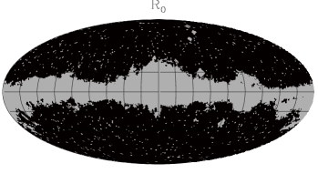
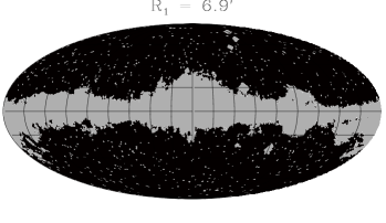
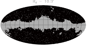
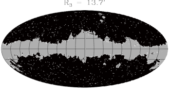
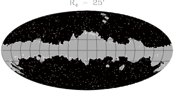
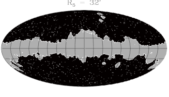
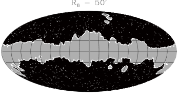
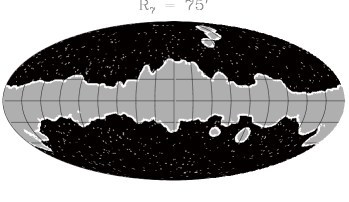
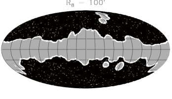
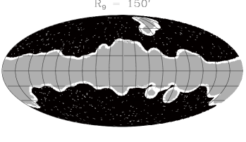
We should take into account the effect of the mask in the wavelet coefficient maps. Pixels near the border of the mask (the Galactic cut and other features) are affected by the zero value of the mask (Vielva et al., 2004). Therefore we need one extended mask for each scale that removes these affected pixels from the analysis. We use the method described in McEwen et al. (2005) to construct our extended masks. We compute the wavelet coefficients at each scale of the 75 mask without the holes corresponding to the point sources, and consider only the pixels with low values (that is, the less affected pixels). Then we multiply by 75 to mask out the point sources. In particular, our threshold is 0.001, i.e., all the pixels which have a wavelet coefficient for the 75 mask larger than 0.001 in absolute value are masked out. In addition we also test the effect of the extension of the mask by applying a less restrictive threshold of 0.01. In Fig. 1 we present the masks that we use for the 10 considered scales.
We also need Gaussian and non-Gaussian simulations for this analysis. The Gaussian simulations are performed as follows. For a given power spectrum (we use the best fit power spectrum for WMAP provided by LAMBDA), we generate a set of Gaussian . From these multipoles we produce a map for each different radiometer by convolving with the corresponding beam transfer function. We also include the pixel properties by convolving with the pixel transfer function. We add a Gaussian noise realisation to each radiometer simulation and then we combine them in the same way as the data maps. Following the analysis of the WMAP team, we assume that the instrumental noise is well approximated by Gaussian white noise at each pixel. This noise is characterised by a dispersion that depends on the pixel position and the corresponding radiometer. Although the data also contain small residuals of noise (Jarosik et al., 2003; Jarosik et al., 2007) their contribution here is expected to be negligible.
The non-Gaussian simulations are produced following a model which introduces a quadratic term in the primordial gravitational potential (Salopek & Bond, 1990; Gangui et al., 1994; Verde et al., 2000; Komatsu & Spergel, 2001):
| (9) |
where is a linear random field which is Gaussian distributed and has zero mean. This kind of non-Gaussianity is generated in various non-standard inflationary scenarios (see, e.g. Bartolo et al., 2004). The simulations with are generated following the algorithms described in Liguori et al. (2003, 2007). In particular we have a set of 300 Gaussian simulations in the space, and their corresponding non-Gaussian part . A simulation with a given value of is constructed as
| (10) |
To produce each non-Gaussian WMAP simulation with we transform the multipoles defined in Eq. 10 into each differencing assembly map using the corresponding beam and pixel transfer functions and we add a Gaussian noise realisation. Then, we combine these maps to form the Q+V+W, V+W, Q, V and W combined maps.
3 Results
In this section we present the Gaussianity analysis of the WMAP data using the Q+V+W, V+W, Q, V, and W combined data maps. First we consider the estimators defined in Eqs. LABEL:witowip22 and the statistic given in Eq. 7 and compare the values obtained for the WMAP data with the distribution constructed with Gaussian simulations. Second we constrain the local non-linear coupling parameter using realistic non-Gaussian simulations. Finally we estimate the contribution of the undetected point sources to the best fit value of .
3.1 Analysis of WMAP data
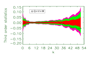
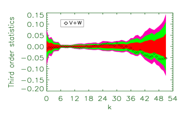
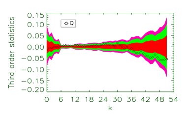
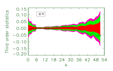
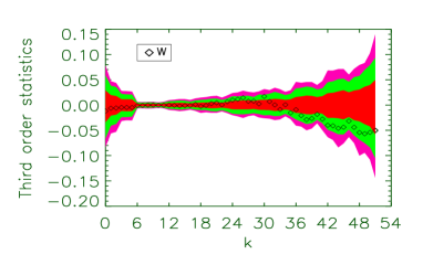
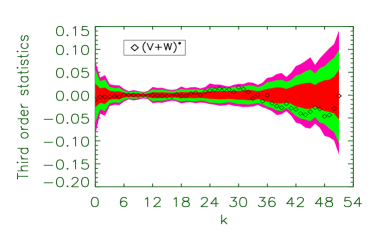


We estimate the wavelet coefficient maps at the 10 considered scales defined in Subsect.2.2. In particular, for we have 52 estimators as the ones defined in Eq. 2.2. In Fig. 2 we present these statistics for the WMAP data compared with the values obtained for 1000 Gaussian simulations. We analyse the Q+V+W, V+W, Q, V, and W combined maps using the restrictive extended masks, and we also analyse the V+W map with the less restrictive extended masks (marked in the tables and figures with ). The estimator (defined in Eq. LABEL:witowip22, corresponding to the skewness) has a similar shape than the one obtained for the 1-year and 3-year data maps (Vielva et al., 2004; Mukherjee & Wang, 2004; Cruz et al., 2007). In all the cases the skewness obtained for the data is compatible with the skewness of Gaussian simulations. We can see in Fig. 2 that the values of the estimators with are systematically below the mean. However, for a correct interpretation of this trend it is important to take into account that those estimators are strongly correlated at large scales. In particular, considering the normalised correlation matrix in the V+W case, , we have that its elements are on average for vector indices greater or equal than 36, whereas for vector indices lower than 36.
We have also performed a analysis in order to check if the data are compatible with Gaussian simulations. This is plotted in Fig. 3. We estimate the mean and the covariance used in Eq. 7 with another set of 1000 Gaussian simulations. We can see that for all the cases, the data are compatible with the Gaussian simulations. The statistical properties of the histograms are presented in Table 1, where we give the value obtained for the data, the degrees of freedom of the statistic (DOF), the mean and the dispersion obtained for Gaussian simulations and the cumulative probability for the data.
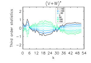
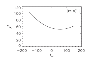
Finally we impose constraints on the parameter using the considered maps. We calculate the expected values of all the estimators for different cases444 We use 300 simulations to calculate the mean values of the estimators for different cases and 1000 Gaussian simulations to calculate the covariance matrix. We analysed the convergence of the mean values by computing the best-fit value of the data using two independent sets of 150 simulations. The difference in the obtained value is lower than 1 and therefore even with 100 simulations the convergence is achieved. Analogously, for the covariance matrix we have checked that convergence is achieved with 1000 Gaussian simulations. (see left panel of Fig. 4 for the combined V+W map). Then, we perform a analysis using Eq. 8 in order to find the best fit value for for each data map. We also analyse Gaussian simulations in order to obtain the frequentist error bars. In the central and right panels of Fig. 4 we present a plot of versus for the combined V+W data and a histogram of the best fit for 1000 Gaussian simulations of the combined V+W map. Table 2 lists the values which best fits the five considered maps, and the main properties of the distributions of best-fit obtained from Gaussian simulations. From this table we have at 95% CL that for the combined V+W map, for Q+V+W, for Q, for V, and for W (using the restrictive extended masks defined in Subsect. 2.3). These values are compatible with the ones obtained by Komatsu et al. (2008) using the bispectrum. Notice that increases as we go from Q to W maps. The value obtained for the V+W map is the same as the one that Komatsu et al. (2008) obtains for this map using and the 75 mask. The Q+V+W map has a smaller value. The best-fit increases with frequency for the Q, V, and W maps, and the of the Q map is larger than the one of the V and W maps. This also agrees with Komatsu et al. (2008).
The less restrictive extended masks give tighter results for the constraints on compared with the restrictive ones. In particular, from Table 2, we have that at 95% CL. In this case the dispersion of is smaller since the available area is larger for all the scales. The additional pixels are not significantly affected by the mask for this analysis and the wavelet is still efficient. These constraints are very similar to those obtained with the bispectrum (Komatsu et al., 2008), which are at 95% CL.
Notice however that other works, e.g. Yadav & Wandelt (2008), have found evidences of non-zero value for at CL using the KSW bispectrum. We do not find deviations with respect to the zero value using the 5-year data at 95 % CL and the same result is presented in Komatsu et al. (2008). We may wonder if that deviation is introduced by the 3-year WMAP mask (Kp0), uncertainties in the characterisation of the beams, or some systematics present in the 3-year data. To check this possibility we analysed the V+W 3-year WMAP data (updated after the 5-year release) using our estimators, the Kp0 mask and its corresponding extended masks. The results are at 95% CL, which are compatible with the 5-year results. Therefore our method is not able to detect the deviations reported in Yadav & Wandelt (2008) using the 3-year data. This may be explained by the fact that the wavelet method probes different combinations of scales than the bispectrum and also responds differently to possible systematics present in the data.
We have also tested other third order estimators that involve the derivatives (in particular the squared modulus of the gradient and the Laplacian) of the wavelet coefficient maps. These estimators are less sensitive to the parameter and its error bars are significantly wider than the ones obtained with the estimators of Eq. LABEL:witowip22.

| Map | DOF | ||||
|---|---|---|---|---|---|
| Q+V+W | 54.65 | 52 | 55.49 | 11.78 | 0.63 |
| V+W | 43.23 | 52 | 55.22 | 11.73 | 0.20 |
| Q | 62.84 | 52 | 55.31 | 12.08 | 0.86 |
| V | 49.81 | 52 | 55.24 | 11.96 | 0.44 |
| W | 41.74 | 52 | 54.92 | 11.34 | 0.16 |
| (V+W)∗ | 55.31 | 52 | 55.47 | 12.47 | 0.65 |
| Map | best | ||||||
|---|---|---|---|---|---|---|---|
| Q+V+W | 26. | -2. | 34. | -34. | 30. | -68. | 67. |
| V+W | 58. | -1. | 33. | -35. | 34. | -66. | 60. |
| Q | 16. | -1. | 42. | -43. | 41. | -79. | 86. |
| V | 30. | 0. | 39. | -39. | 38. | -76. | 79. |
| W | 40. | -4. | 39. | -44. | 35. | -78. | 74. |
| (V+W)∗ | 56. | 0. | 30. | -31. | 30. | -61. | 58. |
3.2 Contribution of undetected point sources
It has been shown that the Mexican hat wavelet is very useful in detecting point sources (Cayón et al., 2000; Vielva et al., 2001) since its contribution is enhanced in the wavelet coefficient maps at certain scales. Therefore it is important to study the contribution of the undetected point sources on the estimation. The skewness and kurtosis of wavelet coefficient maps due to point sources have been studied in Argüeso et al. (2006). We estimate the contribution of the point sources to our estimators by performing Monte Carlo simulations. We use a straightforward model to simulate the radio sources following the one described in Komatsu et al. (2008). In this model it is assumed that all the sources have the same intensity flux, (0.5 Jy), and that they are randomly distributed in the sky following a Poisson distribution. The source contribution to the temperature at any pixel is given by
| (11) |
where , , is a Poisson random variable of mean and is the density of sources. The power spectrum for this type of source distribution can be easily calculated (Tegmark & Efstathiou, 1996).
| (12) |
Using and a pixel resolution of we have a power spectrum of for the Q band. This model roughly reproduces the measured values of the power spectrum and the bispectrum (Nolta et al., 2008; Komatsu et al., 2008).
For this analysis we have performed 1000 point source simulations for the V+W map. We add these point source simulations to the V+W simulations of CMB with noise. For each one we estimate its best fit and compare it with the values obtained for the same simulation but without point sources. The difference gives us an estimate of the contamination due to the point sources. They add a contribution of to the CMB considering the restrictive extended masks. For the less restrictive extended masks the point source contribution is . The difference with the previous result is explained because the zero values of the 75 mask affect the efficiency of the wavelet to detect point sources. This can be seen in the left panel of Fig. 5 where we plot the mean values for the third order estimators for the V+W simulations including point sources for both kinds of extended masks. The mean value of several estimators, specially the skewness for small scales, is lower for the less restrictive extended masks. This reduces the value. Considering the contribution of the point sources, our estimate of for this case is at 68% CL and at 95% CL. For comparison, the bias introduced by point sources for the bispectrum is (Komatsu et al., 2008).
We also estimate the contribution of undetected point sources using the more realistic source number counts , derived from the work of de Zotti et al. (2005). The dependence of with the frequency is very small in the range between 61 GHz and 94 GHz. Thus, for simplicity, we assume the same for both V and W maps, evaluated at a frequency of 71 GHz. We select a range of intensities between 1 mJy and 1 Jy. Then we generate point source simulations following the distribution derived from de Zotti et al. (2005). The simulations are transformed from intensity flux to temperature as in the previous case (following Eq. 11). For this analysis we have also performed 1000 point source simulations for the map and have added them to Gaussian CMB plus noise simulations. We analyse the resultant simulations as in the previous case to obtain the contribution to due to the point sources. They add a contribution of to the CMB considering the less restrictive extended masks and considering the restrictive extended masks. As in the previous case, the differences in using the restrictive and less restrictive extended masks are explained because the zero values of the 75 mask affect the efficiency of the wavelet. This is plotted in the right panel of Fig. 5.
Therefore, considering the realistic point source model and the less restrictive masks our estimate of remains unchanged ( at 95% CL).


4 Conclusions
We have analysed the 5-year WMAP data using Gaussian and realistic non-Gaussian simulations through a wavelet-based test. We have considered different combined maps for the analysis: Q+V+W, V+W, Q, V, and W. We have considered two kinds of extended masks to analyse the V+W map (defined in Subsect. 2.3). The third order moments (Eq. LABEL:witowip22) of the wavelet coefficients of these maps are compatible with Gaussian simulations (see Fig 2).
We have performed a analysis and found that the data are indeed compatible with Gaussian simulations (see Fig. 3). We performed another analysis to constrain the non-linear coupling parameter by using non-Gaussian simulations with . The best-fit values of the five analysed maps are compatible with the ones obtained by Komatsu et al. (2008) using the bispectrum, showing similar confidence intervals and also a similar trend with the frequency.
Finally we have estimated the contribution to from unresolved point sources for the V+W map using a simple model that has point sources with constant intensity ( 0.5 Jy) and a realistic model given by de Zotti et al. (2005). We have found that they add a positive contribution of for the simple model and for the realistic model. These values are larger than the one obtained by Komatsu et al. (2008) for the bispectrum, which can be explained by the enhancement of the point sources produced by wavelets. Using the less restrictive extended masks, the point source distribution add a positive contribution of for the simple model and for the realistic model. The smaller values are explained because the less restrictive extended masks add some pixels that affect the efficiency of the wavelet to detect point sources. Taking into account the point source correction, our best estimate of is at 95% CL. It is important to emphasise the agreement found between the two estimators (bispectrum and wavelets), since they are formed by very different combinations of the data and are affected by systematic effects (like the mask, noise, beam response and foreground residuals) in very different ways.
acknowledgments
The authors thanks J. González-Nuevo for providing the counts and for his useful comments on unresolved point sources. The authors thank P. Vielva and M. Cruz. We also thank R. Marco and L. Cabellos for computational support. We acknowledge partial financial support from the Spanish Ministerio de Ciencia e Innovación project AYA2007-68058-C03-02. A. C. thanks the Spanish Ministerio de Ciencia e Innovación for a pre-doctoral fellowship. A. C. thanks the Astronomy Centre at the University of Sussex for their hospitality during a research stay in 2008. S. M. thanks ASI contract I/016/07/0 ”COFIS” and ASI contract Planck LFI activity of Phase E2 for partial financial support. The authors acknowledge the computer resources, technical expertise and assistance provided by the Spanish Supercomputing Network (RES) node at Universidad de Cantabria. We acknowledge the use of Legacy Archive for Microwave Background Data Analysis (LAMBDA). Support for it is provided by the NASA Office of Space Science. The HEALPix package was used throughout the data analysis (Górski et al., 2005).
References
- Albrecht & Steinhardt (1982) Albrecht A., Steinhardt P. J., 1982, Physical Review Letters, 48, 1220
- Antoine & Vandergheynst (1998) Antoine J.-P., Vandergheynst P., 1998, Journal of Mathematical Physics, 39, 3987
- Argüeso et al. (2006) Argüeso F., Sanz J. L., Barreiro R. B., Herranz D., González-Nuevo J., 2006, MNRAS, 373, 311
- Barreiro et al. (2000) Barreiro R. B., Hobson M. P., Lasenby A. N., Banday A. J., Górski K. M., Hinshaw G., 2000, MNRAS, 318, 475
- Bartolo et al. (2004) Bartolo N., Komatsu E., Matarrese S., Riotto A., 2004, Phys. Rep., 402, 103
- Bennett et al. (2003) Bennett C. L., Hill R. S., Hinshaw G., Nolta M. R., Odegard N., Page L., Spergel D. N., Weiland J. L., Wright E. L., Halpern M., Jarosik N., Kogut A., Limon M., Meyer S. S., Tucker G. S., Wollack E., 2003, ApJS, 148, 97
- Cabella et al. (2005) Cabella P., Liguori M., Hansen F. K., Marinucci D., Matarrese S., Moscardini L., Vittorio N., 2005, MNRAS, 358, 684
- Cayón et al. (2005) Cayón L., Jin J., Treaster A., 2005, MNRAS, 362, 826
- Cayón et al. (2003) Cayón L., Martínez-González E., Argüeso F., Banday A. J., Górski K. M., 2003, MNRAS, 339, 1189
- Cayón et al. (2000) Cayón L., Sanz J. L., Barreiro R. B., Martínez-González E., Vielva P., Toffolatti L., Silk J., Diego J. M., Argüeso F., 2000, MNRAS, 315, 757
- Cayón et al. (2001) Cayón L., Sanz J. L., Martínez-González E., Banday A. J., Argüeso F., Gallegos J. E., Górski K. M., Hinshaw G., 2001, MNRAS, 326, 1243
- Copi et al. (2006) Copi C. J., Huterer D., Schwarz D. J., Starkman G. D., 2006, MNRAS, 367, 79
- Copi et al. (2004) Copi C. J., Huterer D., Starkman G. D., 2004, Phys. Rev. D, 70, 043515
- Creminelli et al. (2006) Creminelli P., Nicolis A., Senatore L., Tegmark M., Zaldarriaga M., 2006, Journal of Cosmology and Astro-Particle Physics, 5, 4
- Cruz et al. (2007) Cruz M., Cayón L., Martínez-González E., Vielva P., Jin J., 2007, ApJ, 655, 11
- Cruz et al. (2005) Cruz M., Martínez-González E., Vielva P., Cayón L., 2005, MNRAS, 356, 29
- Cruz et al. (2007) Cruz M., Turok N., Vielva P., Martínez-González E., Hobson M., 2007, Science, 318, 1612
- Curto et al. (2007) Curto A., Aumont J., Macías-Pérez J. F., Martínez-González E., Barreiro R. B., Santos D., Désert F. X., Tristram M., 2007, A&A, 474, 23
- Curto et al. (2008) Curto A., Macías-Pérez J. F., Martínez-González E., Barreiro R. B., Santos D., Hansen F. K., Liguori M., Matarrese S., 2008, A&A, 486, 383
- De Troia et al. (2007) De Troia G., Ade P. A. R., Bock J. J., Bond J. R., Borrill J., Boscaleri A., Cabella P., Contaldi C. R., et al. 2007, ApJL, 670, L73
- de Zotti et al. (2005) de Zotti G., Ricci R., Mesa D., Silva L., Mazzotta P., Toffolatti L., González-Nuevo J., 2005, A&A, 431, 893
- Eriksen et al. (2005) Eriksen H. K., Banday A. J., Górski K. M., Lilje P. B., 2005, ApJ, 622, 58
- Eriksen et al. (2004) Eriksen H. K., Hansen F. K., Banday A. J., Górski K. M., Lilje P. B., 2004, ApJ, 605, 14
- Gangui et al. (1994) Gangui A., Lucchin F., Matarrese S., Mollerach S., 1994, ApJ, 430, 447
- Górski et al. (2005) Górski K. M., Hivon E., Banday A. J., Wandelt B. D., Hansen F. K., Reinecke M., Bartelmann M., 2005, ApJ, 622, 759
- Gott et al. (2007) Gott J. R., Colley W. N., Park C.-G., Park C., Mugnolo C., 2007, MNRAS, 377, 1668
- Guth (1981) Guth A. H., 1981, Phys. Rev. D, 23, 347
- Hikage et al. (2008) Hikage C., Matsubara T., Coles P., Liguori M., Hansen F. K., Matarrese S., 2008, MNRAS, 389, 1439
- Jarosik et al. (2003) Jarosik N., Barnes C., Bennett C. L., Halpern M., Hinshaw G., Kogut A., Limon M., Meyer S. S., Page L., Spergel D. N., Tucker G. S., Weiland J. L., Wollack E., Wright E. L., 2003, ApJS, 148, 29
- Jarosik et al. (2007) Jarosik N., Barnes C., Greason M. R., Hill R. S., Nolta M. R., Odegard N., Weiland J. L., Bean R., et al. 2007, ApJS, 170, 263
- Jeong & Smoot (2007) Jeong E., Smoot G. F., 2007, [arXiv:0710.2371]
- Komatsu et al. (2008) Komatsu E., Dunkley J., Nolta M. R., Bennett C. L., Gold B., Hinshaw G., Jarosik N., Larson D., Limon M., Page L., Spergel D. N., Halpern M., Hill R. S., Kogut A., Meyer S. S., Tucker G. S., Weiland J. L., Wollack E., Wright E. L., 2008, accepted by ApJS, [arXiv:0803.0547]
- Komatsu et al. (2003) Komatsu E., Kogut A., Nolta M. R., Bennett C. L., Halpern M., Hinshaw G., Jarosik N., Limon M., Meyer S. S., Page L., Spergel D. N., Tucker G. S., Verde L., Wollack E., Wright E. L., 2003, ApJS, 148, 119
- Komatsu & Spergel (2001) Komatsu E., Spergel D. N., 2001, Phys. Rev. D, 63, 063002
- Komatsu et al. (2002) Komatsu E., Wandelt B. D., Spergel D. N., Banday A. J., Górski K. M., 2002, ApJ, 566, 19
- Liguori et al. (2003) Liguori M., Matarrese S., Moscardini L., 2003, ApJ, 597, 57
- Liguori et al. (2007) Liguori M., Yadav A., Hansen F. K., Komatsu E., Matarrese S., Wandelt B., 2007, Phys. Rev. D, 76, 105016
- Linde (1982) Linde A. D., 1982, Physics Letters B, 108, 389
- Linde (1983) Linde A. D., 1983, Physics Letters B, 129, 177
- Martínez-González (2008) Martínez-González E., 2008, [arXiv:0805.4157]
- Martínez-González et al. (2002) Martínez-González E., Gallegos J. E., Argüeso F., Cayón L., Sanz J. L., 2002, MNRAS, 336, 22
- McEwen et al. (2005) McEwen J. D., Hobson M. P., Lasenby A. N., Mortlock D. J., 2005, MNRAS, 359, 1583
- Monteserín et al. (2008) Monteserín C., Barreiro R. B., Vielva P., Martínez-González E., Hobson M. P., Lasenby A. N., 2008, MNRAS, 387, 209
- Mukherjee et al. (2000) Mukherjee P., Hobson M. P., Lasenby A. N., 2000, MNRAS, 318, 1157
- Mukherjee & Wang (2004) Mukherjee P., Wang Y., 2004, ApJ, 613, 51
- Nolta et al. (2008) Nolta M. R., Dunkley J., Hill R. S., Hinshaw G., Komatsu E., Larson D., Page L., Spergel D. N., Bennett C. L., Gold B., Jarosik N., Odegard N., Weiland J. L., Wollack E., Halpern M., Kogut A., Limon M., Meyer S. S., Tucker G. S., Wright E. L., 2008, accepted by ApJS, [arXiv:0803.0593]
- Pando et al. (1998) Pando J., Valls-Gabaud D., Fang L. Z., 1998, Physical Review Letters, 81, 4568
- Salopek & Bond (1990) Salopek D. S., Bond J. R., 1990, Phys. Rev. D, 42, 3936
- Spergel et al. (2007) Spergel D. N., Bean R., Doré O., Nolta M. R., Bennett C. L., Dunkley J., Hinshaw G., Jarosik N., et al. 2007, ApJS, 170, 377
- Tegmark & Efstathiou (1996) Tegmark M., Efstathiou G., 1996, MNRAS, 281, 1297
- Verde et al. (2000) Verde L., Wang L., Heavens A. F., Kamionkowski M., 2000, MNRAS, 313, 141
- Vielva et al. (2004) Vielva P., Martínez-González E., Barreiro R. B., Sanz J. L., Cayón L., 2004, ApJ, 609, 22
- Vielva et al. (2001) Vielva P., Martínez-González E., Cayón L., Diego J. M., Sanz J. L., Toffolatti L., 2001, MNRAS, 326, 181
- Vielva et al. (2007) Vielva P., Wiaux Y., Martínez-González E., Vandergheynst P., 2007, MNRAS, 381, 932
- Wiaux et al. (2008) Wiaux Y., Vielva P., Barreiro R. B., Martínez-González E., Vandergheynst P., 2008, MNRAS, 385, 939
- Wiaux et al. (2006) Wiaux Y., Vielva P., Martínez-González E., Vandergheynst P., 2006, Physical Review Letters, 96, 151303
- Yadav & Wandelt (2008) Yadav A. P. S., Wandelt B. D., 2008, Physical Review Letters, 100, 181301