INSTITUT NATIONAL DE RECHERCHE EN INFORMATIQUE ET EN AUTOMATIQUE
Robust model identification of actuated vortex wakes
Jessie Weller
— Edoardo Lombardi††footnotemark:
— Angelo Iollo††footnotemark:
N° 6559
Juin 2008
Robust model identification of actuated vortex wakes
Jessie Weller††thanks: IMB - Université Bordeaux et MC2 - INRIA Bordeaux Sud-Ouest, 33405 Talence, France , Edoardo Lombardi00footnotemark: 0 , Angelo Iollo00footnotemark: 0
Thème NUM — Systèmes numériques
Équipe-Projet MC2
Rapport de recherche n° 6559 — Juin 2008 — ?? pages
Abstract: We present a low-order modeling technique for actuated flows based on the regularization of an inverse problem. The inverse problem aims at minimizing the error between the model predictions and some reference simulations. The parameters to be identified are a subset of the coefficients of a polynomial expansion which models the temporal dynamics of a small number of global modes. These global modes are found by Proper Orthogonal Decomposition, which is a method to compute the most representative elements of an existing simulation database in terms of energy. It is shown that low-order control models based on a simple Galerkin projection and usual calibration techniques are not viable. They are either ill-posed or they give a poor approximation of the solution as soon as they are used to predict cases not belonging to the original solution database. In contrast, numerical evidence shows that the method we propose is robust with respect to variations of the control laws applied, thus allowing the actual use of such models for control.
Key-words: reduced order models, control, inverse problems
Identification robuste de sillages tourbillonnaires controllés
Résumé : Nous proposons une méthode de réduction de modèle, pour des écoulements actionnés, basée sur la régularisation d’un problème inverse. Le problème inverse vise à minimiser l’erreur entre les prédictions du modèle et des simulations de référence. Les paramètres à identifier sont les coefficients d’une expansion polynomiale qui modélise les dynamiques temporelles d’un nombre limité de modes globales. Ces modes sont obtenus par Décomposition Orthogonale aux valeurs Propres (POD). Il s’agit d’une méthode pour calculer les éléments les plus représentatifs, en termes d’énergie, d’une base de données de simulations. Il est montré que des modèles basés sur une simple projection de Galerkin et sur des techniques classiques de calibration ne sont pas viables. Ils sont soit mal posés, soit donnent une approximation erronée de la solution dès qu’ils sont utilisés pour prédire des dynamiques n’appartenant pas à la base de données originale. En revanche, des évidences numériques montrent que la méthode que nous proposons permet de construire des modèles robustes, qui réagissent correctement à des variations de paramètres, et pourraient donc tre utilisés pour des problèmes de contrôle d’écoulement.
Mots-clés : modèles réduits, contrôle, problèmes inverses
1 Introduction
We consider the problem of describing the dynamics of an infinite
dimensional system using a small number of degrees of freedom. In
particular we concentrate on the problem of devising accurate and
robust models of actuated fluid flows past bluff obstacles. These
flows are dominated by the presence of large-scale vortices due to
massive separation, and are good candidates for a low-dimensional
representation. The point of view that we privilege is empiric: the
functional space in which we seek the low-dimensional solution is
derived using proper orthogonal decomposition (POD) L67 . POD
makes use of simulation databases to determine optimal functional
spaces in terms of solution representation. A vast literature
concerning this way of modeling fluid flows exists
Galletti2006 ; Buffoni2006 ; Galletti2004 ; MK02 , and some results
show the possible interest of using POD in applications such as flow
control B06 ; G98 ; GR98 .
However, several problems related to the idea of modeling a flow by a
small number of variables are open. One of the issues is the
asymptotic stability of the models obtained. Often such models are
capable of correctly reproducing the dynamics over small time
intervals, whereas the asymptotic behavior converges to incorrect
limit cycles MK02 . This issue is related to both numerical
artifacts and to an improper representation of the
solution Iollo2000 ; rempfer2000 ; Noack . As a results low-order models
are of delicate use and not robust to parameter variations.
The present study describes a method to obtain robust low-order
models. In previous works we showed that it is possible to obtain
accurate low-order models of relatively complicated flows by
minimizing the error between the model results and the reference
solution Buffoni2006 . Here we extend those works to cases where
the flow is actuated by devices that can affect locally or globally the
velocity and pressure fields. The objective is to derive a low-order
model that provides accurate predictions and that is robust to
variations of the control law employed. The main idea is to identify
the manifold over which the non-linear dynamics of the POD modes lies,
when the input to the system is varied. In this spirit, several
dynamics are included in the identification procedure coupled with a
Tikhonov type regularization. The case of a precomputed control as
well as the case of a feed-back control are studied.
The practical relevance of this work is that low-order models make
possible to devise or to optimize controls for large-scale problems
that would not be otherwise solvable in terms of computational
size. Applications of this method is straight forward for models other
than the Navier-Stokes equations.
2 Reduced Order Modeling using POD
2.1 Flow setup
We consider a two-dimensional laminar flow past a confined square cylinder. This setup presents a reasonable compromise between physical complexity and computational cost. A sketch showing the geometry, the frame of reference and the adopted notation is plotted in Fig.1.

At the inlet, the incoming flow is assumed to have a Poiseuille
profile with maximum center-line velocity . With reference to
Fig.1, , , . No-slip conditions are enforced both on the cylinder and on the
parallel walls. Details concerning the grids and the numerical set up
are reported in Buffoni2006 .
All the quantities mentioned in the following have been made
non-dimensional by and . The two-dimensional unforced flow
obtained is a classic vortex street with a well defined shedding
frequency. The interaction with the confining walls leads to some
peculiar features, like the fact that the vertical position of the
span-wise vortices is opposite to the one in the classic von
Kármán street Camarri2006 .
The presence of an actuator is modeled by imposing a new boundary
condition on a small surface of :
For control purposes we place two actuators on the cylinder. They are driven in opposite phase, as shown in Fig. 2:
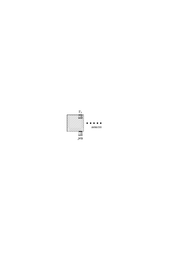
The control law can be precomputed, or obtained using a proportional feedback law. For example, using measurements of the vertical velocity at points in the cylinder wake, we can define a proportional control law:
where denotes the number of sensors used.
2.2 Proper Orthogonal decomposition with the snapshot method
Seeking a reduced order solution that can be written
where the spatial functions are obtained by POD has become a popular approach when dealing with large scale systems. A vast literature concerning the POD procedure exists Holmes , we refer to these works for a more general review of the method.
2.2.1 The POD basis
In our case, a numerical simulation of the Navier-Stokes equations is performed over a time interval , and the velocity field is saved at time instants . This yields a data set . The aim of the POD procedure is to find a low dimensional subspace of , that gives the best approximation of . We therefore seek an orthonormal set , where , and a set of coefficients such that the reconstruction error:
| (1) |
is minimal.
Following Sirovich’s idea S87 the POD modes are expressed as
linear combinations of the snapshots:
The vectors are found to be the
eigenvectors of the correlation matrix , , corresponding to the highest eigenvalues, while
the are equal to the scalar products .
In the case of forced flow, the snapshots depend on the control law
used. In this work we consider POD basis derived from numerical
simulations obtained using several different control laws. Indeed,
there are a number of other parameters that could be varied, but since
our aim is to study the effect of a control law, we set ourselves in
the following framework:
-
–
Time instants, Reynolds number, domain geometry, placement of the actuators will be the same for all the snapshots in the database.
-
–
The control law will be varied
The data set used for the POD is therefore written:
where denotes the number of control laws considered. If is the set of control laws used to obtain the database, the ensuing POD basis is denoted . In the first part of this work, is reduced to a single element which we denote .
2.2.2 Dealing with the boundary conditions
In the non-controlled case, we lift the boundary conditions on the velocity fields by defining a new set of snapshots:
where is some reference velocity field that satisfies the same
boundary conditions as the snapshots. In the present configuration, it
can be the steady unstable solution, or a time average of the
snapshots .
When an extra boundary condition is imposed on the cylinder for
control purposes, the snapshots are chosen to be:
where satisfies the following criteria:
In practice we use the velocity field proposed in Galletti2006 :
where is obtained in the same way as but applying a constant control equal to on . The low-dimensional solution is now written:
| (2) |
2.3 POD-Galerkin Reduced Order Model
Galerkin projection of the incompressible Navier-Stokes equations onto the first POD modes yields a system of ordinary differential equations:
| (8) |
where:
We note that since the snapshots satisfy the continuity equation, the
modes do also. This implies that the pressure term is equal
to . If velocity field is constant
at the boundaries, the POD modes are zero there. The pressure term
therefore disappears completely.
Setting:
and
the first equation in (8) can be written in the compact form:
The initial value problem (8) is a reduced order model of the Navier-Stokes equations, called the POD-Galerkin model. Such a model might be inaccurate for it may not take into account enough of the dynamics. Indeed, although a number of modes can be sufficient to capture most of the flow energy, the neglected modes continue to play an important role in the flow dynamics through their interaction with the conserved ones. The difference between the solutions of (8), and the coefficients obtained by projecting the numerical data onto the POD modes (), has been underlined in several papers Galletti2006 ; B06 ; Couplet2005 . It is therefore interesting to build a model that exploits the knowledge one has of the dynamics, that is the set of temporal projection coefficients . This is the subject of the next section.
3 Robust low order models
3.1 Calibration method
The idea of calibration is to keep the structure of the above model while adjusting the coefficients of the system so its solution is closer to the desired one. In previous work Galletti2004 ; Galletti2006 , it was shown that robust low order models could be obtained by solving the minimization problem:
| (11) |
This state calibration method, which involves solving a
strongly non-linear system, works well as long as the number of
snapshots considered remains limited. For a large number of snapshots,
the computational costs are excessive.
Another method was suggested in Galletti2004 , and has been
experimented, for a case with no control, in
Buffoni2006 ; Buffoni2008 ; Couplet2005 with good results. It
consists in choosing as the solution of:
| (12) |
This method can be interpreted as approximating the error
by a quadratic function of all the non-discarded temporal
coefficients, and . Other choices for the
approximation of lead to partial calibration problems.
For example, if we suppose then we will solve:
| (13) |
where
and
Of course, other choices of which terms to calibrate or not can be made. For a general formulation we denote the number of terms of vector that are calibrated, and we have . Whatever the choice for , this approach is always much more efficient than (11) since it involves solving linear symmetric systems of size :
| (19) |
The more terms of are calibrated, the more the problem
becomes ill-conditioned. For this reason we choose not to calibrate
the terms .
Once the model has been calibrated to fit a particular control law , it can of course be integrated using another control law. Denoting the input control law , the calibrated model is written:
| (24) |
where by denoting the model we put in evidence that it was calibrated using the control .
3.2 Well-posedness and robustness
3.2.1 Calibration with feedback control laws
We suppose that the control is obtained using a proportional feedback law (Sec.2.1):
We can now consider two different calibration problems. The first is the problem (12), the second is:
| (25) |
where is defined by:
| (26) |
This last approach makes the reduced order model a feedback model,
which is useful if we want to use the model to determine an optimal
feedback law. The problem is however under-determined.
We reformulate (26) to clearly show the dependency of on
:
| (27) |
where
We now look at the partial-calibration problem described above. The function that appears in system (19) can be reformulated:
System (19) is therefore rank deficient. The problem
remains if more of the system coefficients are calibrated, and
according to the choice made the rank of the problem matrix can even
diminish with respect to .
This difficulty can however be solved by using one of the two methods
proposed in the section (3.3). Finally, the proportional
feedback reduced order model is written:
| (33) |
3.2.2 Instability issues
The system solved for calibration can be ill-posed even in cases different to the one just described. To understand why this is, it is sufficient to go back to the state calibration method mentioned at the beginning of the section. Solving the minimization problem (11) involves solving a non-linear system for which the uniqueness of solution is not guaranteed. The state calibration functional can therefore have several local optima, and so there are several possible choices for that will lead to a low value of the error . Since these choices should also be good choices for the minimization problem (13), the matrix in (19) is in general almost singular. A model obtained by inverting this matrix is most often very unstable. To overcome this problem we propose a Tikhonov type regularization method which we describe in the next section.
3.2.3 Robustness
While a calibrated reduced order model works well when
integrated with , its behavior when integrated with a
different control law is unpredictable. As such, the reduced order
model can difficultly be used for estimation and optimization
purposes.
In the literature several methods are proposed for adapting reduced
order modeling for control purposes, some successful examples can be
found in Hinze2005 ; Rav2007 ; Berg2008 . However for those cases,
no calibration seems necessary for the models to work, but this is not
the case for general control problems as shown in the following.
The originality of the model we propose hereafter, is the combination
of multi control data sets with the calibration procedure. Such a
model is fast to build and yet remains accurate for different control
inputs.
3.3 Building a robust low order model
In this section we describe a method to make the reduced order model stable and robust.
3.3.1 Tikhonov regularization
Correctly solving (11) can be done by applying a quasi-Newton method, initialized with and . It therefore seems reasonable to solve the following regularized problem, instead of (13):
| (37) |
where is the regularization parameter.
The parameter can be chosen by a classical technique. We
start by plotting, for a set of values of in
, the error versus the coefficient variation . This leads to a classical Tikhonov L-shaped curve of
which the corner point is optimal in the sense that it is a good
compromise between the error on the dynamics and the distance from
the original coefficients Hansen . The value of
corresponding to this point can be chosen to perform the calibration
procedure.
3.3.2 Calibrating over more than one control law
In this paragraph we look at the changes to be made to the reduced order model when the data set includes simulations obtained using different control laws. Letting:
the calibration problem becomes:
| (38) |
We remark that although the size of the snapshots database is proportional to
the number of controls considered, the size of the calibration problem
remains constant. Furthermore, if the rank deficiency
discussed for proportional feedback no longer occurs.
The main idea is that as the number of controls is increased,
although the model can become a little less precise for the reference
control, it is much more accurate for other control laws. In
the next section we show some successful examples of this method at
different Reynolds number, and for different kinds of control laws.
We refer to a model built using control laws as an -control
model. Such a model is denoted where .
4 Results and discussion
The described technique was applied in order to build a low order
model of the actuated flow around the confined square cylinder in
various configurations. We tested the prediction capabilities of the
model for two different Reynolds number, and ,
with precomputed and feedback control laws. In particular we built
different models with one and more control laws and we analyzed their
predictions with different controls.
In all the examples presented in the following, actuation is started
only once the flow is fully developed. With the control turned on the
simulation is performed for about seven vortex shedding cycles, and
snapshots are saved. is the
non-dimensional duration of the time interval. The number of POD modes
retained for the reduced order model is for the case
and for the case .
We measure the accuracy of the model in the following
way:
-
–
Time coefficients dynamics:
For a given value of , plot , solution of with input , against , projection of the full order solution onto the POD basis . In the examples is usually chosen because it was the mode for which the differences between models were the most remarkable. -
–
Computation of the integration error:
where
In the examples with feedback laws we use only one sensor placed in
the cylinder wake. Choosing the center of the cylinder as the origin
of a coordinate system, we denote the position of
the sensor. The integration error is
measured in the same way as for the non-feedback case.
Our first goal is that the model should be able to reproduce the DNS
data to which is was fitted, we therefore expect
to be small if . Our
second goal is that the model be robust to parameter variation. As the
difference between and the controls in increases,
the error grows. We seek a model for which
this growth rate is as low as possible.
4.1 Divergence of a classical Reduced Order Model
A simulation at was performed using feedback control with a
sensor placed at and . We denote
the control law obtained at the end of simulation.
We compare the results obtained with the POD Galerkin model
(8) and with the calibrated model
(see system (24) for model formulation).
The model integration error is equal to for
the non-calibrated model, and to for the calibrated model.
For a feedback model, the difference is even more important. We
integrated the feedback system (33) with , once with
obtained by Galerkin projection, and once with calibrated
as described in 3.2.1. We obtained an integration error
of in the first case, against an
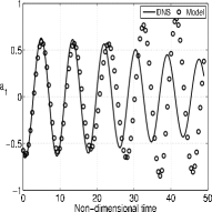
error of in the other. An example of the errors in terms of time
dynamics that the non-calibrated model can produce are shown in
Fig.3.

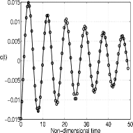
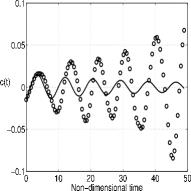
In Fig.4 we plot the control law computed when
integrating the feedback model, and on the same figure, the original
control law . Results for the non-calibrated case are plotted on
the right: the distance between and increases with
time, meaning that at each time step, new errors are added to
the model. Calibration is therefore all the more essential when considering
feedback control.
In order to calibrate, regularization is needed to get well-conditioned
inverse problems as shown in the following. However, the
choice of the parameter is not an easy one.
For example, we performed a simulation at using a feedback
control with a sensor placed at and
. The calibration described in 3.3.1 was performed
with . This led to an ill-conditioned system to
solve and to a model that was not very accurate, and not robust at all
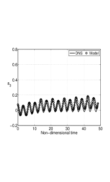
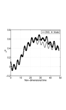
to parameter variations. The effect of on model results is
shown in Fig.5. The two top figures show the
third modal coefficient obtained by projection and by integrating the
model with . On the left, we plot the results obtained when
the model was built with : at the end of the
time period the model diverges from the DNS results. With a higher
value, , this problem no longer occurs, as shown on
the right. The same test was then performed with a different value of
in order to see the models capacity to predict dynamics to which
it was not fitted. The results are shown in the same figure:
divergence was immediate for a low value of , whereas for a
higher value, the model, although not accurate, was at least stable.

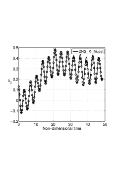
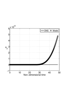

It appears that, when using an higher regularization parameter, the calibration system is well conditioned, the model more accurate and more stable when integrated with a different control law to those used for calibration. In the following the parameter is determined using the L-method with the restriction that any values of below a certain threshold are excluded.
4.2 Testing model robustness
In this section we present the improvements brought to model robustness by introducing calibration over several control laws. For both Reynolds numbers, and , the same experiment was performed:
Step 1 : Build 1- , 2- and 3-control models
We started by choosing three control laws which we denote , and . For each control we performed a simulation of the Navier-Stokes equations, saving snapshots for each simulation. We then defined seven control sets:
For each control set , we computed a POD basis
as described in section 2.2.1 and a
calibrated reduced order model by solving problem
(38).
In the following we refer to , and
as the model control laws.
Step 2 : Run the model with different control laws
We next chose several other control laws which we denote
. Each of these test control laws was used as
input for the Navier-Stokes equations, and for the seven reduced order
models described above. The snapshots from the
Navier-Stokes simulations were projected onto the seven POD bases
. This procedure made it possible to compute the
model integration errors ,
and compare the efficiency of each model.
For measuring model robustness, it is useful to have some idea of how
much the dynamics we are trying to predict, differ from those included
in the model. We therefore need to find a way, for each model, to
measure the distance between the snapshots that were
used to build it, and the snapshots obtained using a
test control law. To do this we proceed in the following way
: if the control set is composed of control laws, then
the distance between the simulations associated to
, and the one obtained using , is defined as:
where the terms ( or ) result from
projecting the snapshots onto the POD basis .
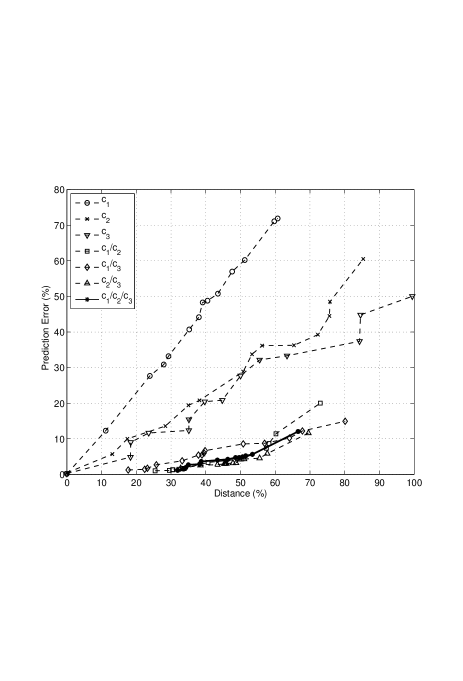
The results are plotted for in Fig. 8 and
Fig. 12. For each value of model , the model
integration error is plotted versus the distance
. We note that the three controls used to build the
models were in fact included in the test set, which explains why there
are 3 points at .
4.3 Results for
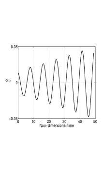
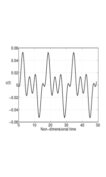
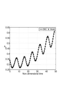
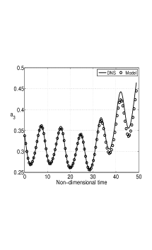
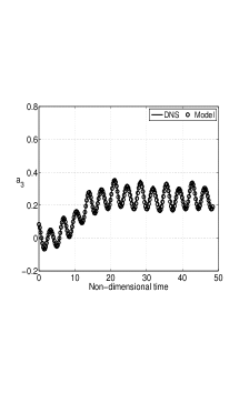
In Fig.6 we plot the control laws used to build the models. For each control law we plot the third modal coefficient to give an idea of the dynamics induced. The figure also shows the prediction for this coefficient given by the 3-control model . The model results are accurate: the reduced order model was successfully calibrated to fit several dynamics.
![[Uncaptioned image]](/html/0806.2748/assets/x11.png)
![[Uncaptioned image]](/html/0806.2748/assets/x12.png)
![[Uncaptioned image]](/html/0806.2748/assets/x13.png)
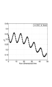
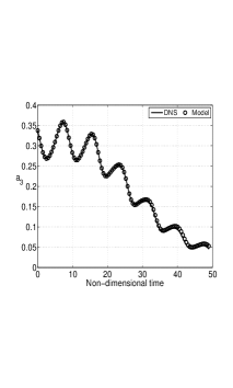

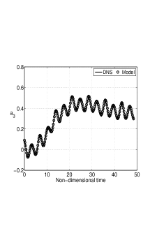
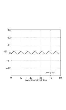
Eleven extra control laws were used for testing. A few examples are
plotted in Fig. 7. For these examples we also plot the
third modal coefficient obtained by projection and by model integration.
Some discrepancies in coefficient amplitude are
observed, but overall the model predicts the right time dynamics.
In Fig. 8 we look at the results obtained with the
different models, using the distances and errors described
above. The first point to be made is that the
model error is almost zero when the distance from the model is
zero. This confirms that 1-control models work well when integrated
with the control law to which they were fitted. The errors then
increase with the distance from the model, as was expected.
The graph highlights the disadvantage of 1-control models. In the
best case the difference between projection and prediction
coefficients becomes higher than 20% as soon as the distance from the
model exceeds 40%. In contrast, for the 2-control and 3-control
models, the error stays under 20%, even when the distance increases.




In Fig. 9 we plot isolines of the vorticity at time for one of the test control laws (the third control law in Fig.7). Time coefficients were obtained by solving with . The velocity field was then reconstructed using the first ten of these coefficients and the first ten POD modes in . The reconstructed vorticity is presented along with the vorticity obtained by running the Navier-Stokes equations with the test control law. The controls used to build the model caused a slight decrease in vortex size (see Fig. 6, bottom left) whereas actuation used in the test caused a slight increase in vortex size (see Fig. 7, bottom right) . We note that the model was able to predict such features, and that at the end of the simulation time, the structure of reconstructed flow is almost identical to that of the real flow. In contrast, the 1-controls weren’t able to identify this. If the same reconstruction is performed using for example, the flow appears almost stable at , meaning the model predicted the opposite behavior to what actually happened.
4.4 Results for
For only feedback control laws are used both to build the models and to perform the tests. In Fig.10 the three feedback control laws used to calibrate the model are shown. The laws are obtained with sensors placed at and by using gains , and . The figure also shows the third modal coefficients given by integrating the 3-control feedback model with each gain. Although the control laws induce different dynamics, the model is able to give an accurate prediction in all three cases.



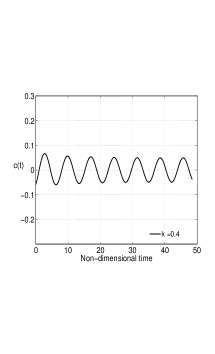
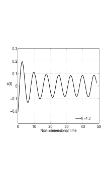

Six extra control laws were used for testing, each corresponding to a different choice of . A few examples, with corresponding coefficients are plotted in Fig.11. It appears that the dynamics are quite different when the distance, between the gain value and gains included in the model, is large. For example, when using a gain the average value of is low compared to that obtained with . However, the 3-control model again gives an overall good prediction of the time dynamics.
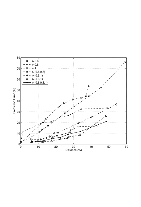


Fig.12 is built the same way as
Fig. 8. In particular the graph shows the disadvantage
of using a 1-control model, with prediction errors of over when
the distance from the calibration dynamics increases over the
. As in the case , the 2-control models give more
accurate predictions than the 1-control models. The lowest errors are
obtained with the 2-control model . This
observation suggests that, in model construction, an optimized a
priori choice of the sampling points could be useful to obtain a more
robust model. We note that in this case it was the model built to fit
the highest and lowest values of that gave the best result, and
that adding a third intermediate control to the model () did
not bring any improvement: the 3-control model gives more or less the
same results.
In Fig. 13 we plot isolines of the vorticity at time
for the flow obtained using as feedback gain (the
first one in Fig.11). Time coefficients were obtained by
integrating the 3-control model. The velocity field was then reconstructed using all
the coefficients and POD modes. The reconstructed vorticity is
presented along with the vorticity obtained by running the Navier-Stokes
equations with the test control law. The controls used to build the
model were similar in the sense that they had a much stronger effect on the
flow compared to the control obtained with . We note that the
model is able to accurately predict a flow snapshot and that the
reconstructed flow is almost identical to that of the real flow.
5 Conclusions
The overall picture of reduced-order modeling that results from our
study is the following. Given a control law, one can deduce a
low-order model of the actuated flow by simply projecting the
Navier-Stokes equations on POD modes. The coefficients of the
quadratic model thus obtained are found by projection. However, a model
constructed this way will show large time-integration errors even for
the same control law used to generate the POD modes. Calibration can take care of
that, in the sense that the model coefficients can be determined in
order to match as closely as possible at least the solution from which
the POD modes are obtained. This might lead to a numerically stable
model. However, this model is generally not at all robust, in the sense
that the predictions for a slightly different configuration from that
it was generated from, fails. A symptom of
such lack of robustness is observed in the ill-posedness of the
inverse problem: the matrices to be inverted are almost singular.
In order to get around this deficiency, we regularize the solution by
adding a constraint to the minimization method used to solve the
inverse problem. We ask that the coefficients of the polynomial
expansion be close enough to those obtained by projection. This
method allows to synthesize models that adequately simulate the flow in
a small vicinity of the control law used to generate the solution
database. However, the actual real improvement in robustness is
obtained by spanning the solution manifold, i.e., by including several
control laws in the inverse problem definition. By doing this, the
results presented show that the models are able to predict dynamical
behaviors that are far, in terms of an energy norm, from the cases
included in the database. A consequence of such an additional
regularization is that the matrices involved in the inverse problem
solution become well conditioned.
Another important aspect of the
method proposed, is that its cost is that of a matrix inversion, and
that it does not scale with the number or the size of data sets used to build
the model. Therefore it seems reasonable to envisage an automatic
strategy to enrich the model by spanning the control space. In this
respect, the technique proposed in Willcox2007 to distribute
in an optimal way the points where to test the control space can help
minimize the number of a priori simulations needed to build the
model. For example, our results show that a model based on two
controls might predict the effect of actuation laws not present in the
data base, as precisely as a model based on three controls, if the two
controls are appropriately placed.
In conclusion, the modeling we propose appears to be a viable approach
to determine control strategies for those problems that because of their
computational size cannot be treated in the framework of classical
control theory.
References
- (1) M. Bergmann and L. Cordier. Optimal control of the cylinder wake in the laminar regime by trust-region methods and pod reduced-order models. J. Comput. Phys., 2008. To appear.
- (2) M. Bergmann, L. Cordier, and J.-P.Brancher. Optimal rotary control of the cylinder wake using proper orthogonal decomposition reduced-order model. Physics of Fluids, 17:097101, 2005.
- (3) M. Buffoni, S. Camarri, A. Iollo, E. Lombardi, and M. V. Salvetti. A non-linear observer for unsteady three-dimensional flows. J. Comput. Phys., 227(4):2626–2643, 2008.
- (4) M. Buffoni, S. Camarri, A. Iollo, and M.V. Salvetti. Low-dimensional modelling of a confined three-dimensional wake flow. Journal of Fluid Mechanics, 569:141–150, 2006.
- (5) T. Bui-Thanh, K. Willcox, and O. Ghattas. Parametric reduced-order models for probabilistic analysis of unsteady aerodynamic applications. Collection of Technical Papers, Vol. 4. AIAA/ASME/ASCE/AHS/ASC, 2007.
- (6) S. Camarri and F. Giannetti. On the inversion of the Kármán street in the wake of a confined square cylinder. J. Fluid Mech., 574:169–178, 2007.
- (7) M. Couplet, C. Basdevant, and P. Sagaut. Calibrated reduced-order pod-galerkin system for fluid flow modelling. J. Comput. Phys., 207(1):192–220, 2005.
- (8) B. Galletti, A. Bottaro, CH. Bruneau, and A. Iollo. Accurate model reduction of transient flows. Europ. J. Mech. / B Fluids, 26:354–366, 2006.
- (9) B. Galletti, C. H. Bruneau, L. Zannetti, and A. Iollo. Low-order modelling of laminar flow regimes past a confined square cylinder. J.Fluid Mech., 503:161–170, 2004.
- (10) E. A. Gillies. Low-dimensional control of the circular cylinder wake. J. Fluid Mech., 371:157–178, 1998.
- (11) W. R. Graham, J. Peraire, and K. Y. Tang. Optimal control of vortex shedding using low-order models. part i. Int. J. Num. Meth. Eng., 44:945–972, 1998.
- (12) P.C. Hansen. Rank-Deficient and Discrete Ill-Posed Problems: Numerical Aspects of Linear Inversion. SIAM, Philadelphia, PA, USA, 1997.
- (13) M. Hinze and S. Volkwein. Proper orthogonal decomposition surrogate models for nonlinear dynamical systems: Error estimates and suboptimal control. Dimension Reduction of Large-Scale Systems, pages 261–306, 2005.
- (14) P. Holmes, J.L. Lumley, and G. Berkooz. Turbulence, Coherent Structures, Dynamical Systems and Symmetry. Cambridge University Press, 1996.
- (15) A. Iollo, A. Dervieux, J. A. Désiéri, and S. Lanteri. Two stable pod-based approximations to the navier-stokes equations. Comput. Visual. Sci., 3:61–66, 2000.
- (16) J. L. Lumley. The structure of inhomogeneous turbulent flows. In Atmospheric Turbulence and Radio Wave Propagation, edited by A. M. Yaglom and V. L. Tatarski, Nauka, Moscow, pages 166–178, 1967.
- (17) X. Ma and G. E. Karniadakis. A low-dimensional model for simulating three-dimensional cylinder flow. J. Fluid Mech., 458:181–190, 2002.
- (18) B.R. Noack, K. Afanasiev, M. Morzynski, G. Tadmor, and F. Thiele. A hierarchy of low-dimensional models for the transient and post-transient cylinder wake. Comp. Meth. Appl. Mech. Eng., 497:335 – 363, 2003.
- (19) S.S. Ravindran. Optimal boundary feedback flow stabilization by model reduction. Comp. Meth. Appl. Mech. Eng., 196:2555–2569, 2007.
- (20) D. Rempfer. On low-dimensional Galerkin models for fluid flow. Theor. Comput. Fluid Dyn., 14:75–88, 2000.
- (21) L. Sirovich. Turbulence and the dynamics of coherent structures. Parts I,II and III. Quarterly of Applied Mathematics, XLV:561–590, 1987.