Uncertainties and shortcomings of ground surface temperature histories derived from inversion of temperature logs

Abstract

Analysing borehole temperature data in terms of ground surface history can add useful information to reconstructions of past climates. Therefore, a rigorous assessment of uncertainties and error sources is a necessary prerequisite for the meaningful interpretation of such ground surface temperature histories. This study analyses the most prominent sources of uncertainty. The diffusive nature of the process makes the inversion relatively robust against incomplete knowledge of the thermal diffusivity. Similarly the influence of heat production is small. It turns out that for investigations of the last 1000 to 100 000 years the maximum depth of the temperature log is crucial. More than 3000 m are required for an optimal inversion. Reconstructions of the last one or two millennia require only modestly deep logs (>300 m) but suffer severely from noisy data.

submitted to Journal of Geophysics and Engineering

1 Introduction

Borehole temperature data record past changes in ground surface temperature (GST) as the transient temperature signal diffuses into the subsurface. These temperature data have been used to reconstruct time series of the ground surface temperature in numerous studies. The value of such reconstructions as a proxy for the paleoclimate, however, is still subject of research and discussion (e.g. Mann & Schmidt 2003). It has been shown (e.g. González-Rouco et al. 2003, Signorelli & Kohl 2004) that surface air temperature (SAT) and soil temperature correlate well at long timescales. Reconstructions have been carried out on various timescales from a few hundred to 100 000 years by several authors. While the shorter type serves, combined with proxy climate data, as a means to investigate natural and anthropogenic climate change, the longer reconstructions study temperatures of the last ice-age and its transition to our current climate.

The problem is usually simplified to a purely conductive, one-dimensional one. If the model fails to capture reality, any inverse method will produce spurious results. Previous studies have already analyzed various effects that can possibly influence the transient signal. For instance, the error introduced by the common assumption of one-dimensionality has been treated by Shen et al. (1995) and Kohl (1999). Advection of heat by groundwater flow can modify the signal considerably (Clauser et al. 1997, Kohl 1998, Taniguchi et al. 1999, Reiter 2005). In the following analysis we will show that even with all simplifying assumptions fulfilled, it is possible to produce artefacts in the inverted time series. Although we use a particular algorithm for the study, the results will more or less apply to other programs as well. We will start with a short review of the theory of the algorithm in the next section.

1.1 Theory

The algorithms commonly used for GST history inversion assume a one-dimensional, purely conductive model. The physical properties of the subsurface are known, the medium can be layered (Shen & Beck 1991, 1992) or is assumed to be homogeneous (Mareschal & Beltrami 1992, Beltrami & Mareschal 1995). Both versions can be used on single boreholes or on ensembles of temperature logs in order to improve the signal to noise ratio. In a comparison of different codes (Beck et al. 1992), it was found that all of them perform equally well under similar circumstances.

In the model considered here (Mareschal & Beltrami 1992, Beltrami & Mareschal 1995), the subsurface is considered homogeneous. The steady state temperature profile is defined by the heat flux at the surface $q_{0}$, the pre-observational mean ground surface temperature $T_{0}$, thermal conductivity $\lambda$, and heat production rate $A$ of the subsurface. Together with a additional transient term $T_{t}(z,t)$ the temperature at time $t$ and depths $z$ is given by (Carslaw & Jaeger 1959, Beltrami & Mareschal 1995):

$$T(z,t)=T_{0}+\frac{q_{0}z}{\lambda}-\frac{Az^{2}}{\lambda}+T_{t}(z,t).$$ (1)

In the particular case that the GST history can be parameterized by stepwise temperature changes $T^{G}_{j}$ at times $t_{j}$ before present ($t=0$) the transient term becomes

$$T_{t}(z)=\sum\limits_{j=1}^{N}{T_{n}^{G}\left({\mbox{erfc}\left({\frac{z}{{2\sqrt{\kappa t_{j}}}}}\right)-\mbox{erfc}\left({\frac{z}{{2\sqrt{\kappa t_{j-1}}}}}\right)}\right)}$$ (2)

If thermal conductivity, diffusivity and heat production are known, the only remaining unknowns are the steady-state GST, the surface heat flow and the values of the the GST history. If temperatures are recorded at depths $z_{i}\quad i=1,...,M$, a set of M linear equations can be formed from equation 1, that can be solved for the unknown variables. The solution needs to be regularized because the problem is ill-posed. The singular value decomposition (Lanczos 1961) is used for this purpose by solving the linear problem and at the same time seeking a solution that minimizes the norm of the model. Implications of this procedure will be discussed in more detail in section 2.

The original code was employed in various case studies for the reconstruction of past climates (e.g. Beltrami et al. 1997, Beltrami & Bourlon 2004, Clauser & Mareschal 1995, Clauser et al. 1997, Jones et al. 1999). It was also used in conjunction with other proxy data to improve the temporal resolution of the GST history as well as the coupling between GST and SAT (Beltrami et al. 1995, Beltrami & Taylor 1995, Signorelli & Kohl 2004, Nitoiu & Beltrami 2005). Before analyzing the sensitivity of this algorithm it is worthwhile to investigate the effect of changing GST on the temperature measured in boreholes.

1.2 Paleoclimate influence on subsurface temperatures

Figure 1: Time and depth scales of GST changes and respective changes in today’s subsurface temperature. Top: Idealized GST history (Haenel et al. 1988, table 10.9). The different line styles mark characteristic periods, respectively. Bottom: Temperature anomalies in the subsurface computed from the time series. Line colours of the anomalies correspond to the periods of the upper panel. The dashed line is equivalent to the sum of the anomalies.

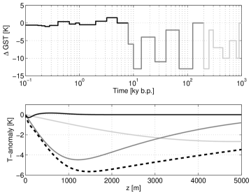
The magnitude and time/depth scale of GST changes can be seen in figure 1. We used a temperature history of the last 1 million years based proxy data (Haenel et al. 1988, table 10.9) to demonstrate the effect of this transient signal on the subsurface temperatures. The curve is valid only for Switzerland but it displays the main features of the climate of the last 1 million years. The proxy curve is subdivided into 3 parts and for each a perturbation with respect to the mean is calculated. The transient signals for each of the periods are computed separately (figure 1, lower panel, solid lines). The mean GST ($T_{0}$ in equation 1) for each of the computations is assumed to be 0°C.

The total transient signal (dashed line) is then the sum of the three partial signals. It is apparent that changes of the order of $10^{6}$ years for this particular GST history will appear in a temperature log as a virtually straight line with a slope of about -1 K km-1 unless the temperature log runs down to a depth of at least 4000 m. The slope will change if a different GST history is used but it is clear that this part of the transient signal cannot be resolved by an inversion, especially not in the presence of noise. Thus, fluctuations of the period 100 000 to 1000 000 years will usually appear only in the pre-observational mean (POM). The glacial temperature minimum and the postglacial temperature increase (100 000 to 10 000 years) cause the most prominent disturbance of the temperature profile. The temperature deviation reaches its maximum amplitude at about 1500 m depth, but still has a value of 1.5 K at 4000 m depth. Because most of the available undisturbed temperature data are from smaller depths, a large portion of this signal is frequently not recorded. The signal due to temperature variations during the Holocene can be traced down to a maximum depth of 1000 m. Although temperature data in this depth range are more numerous, reconstructions have been attempted using substantially shallower data.

From the discussion above two questions arise. Section 2 focuses on the question what the value of the regularizing parameter $\epsilon$ for any given problem should be and whether some objective criterion can be used to define it. In section 3 the question is addressed if a reliable reconstruction of past temperatures is possible when only part of the transient signal is contained in the data.

2 Optimum choice of regularization parameter

It was mentioned in the introduction that a regularization is needed to solve the inverse problem in a stable manner. For the singular value decomposition, two methods are commonly used (Menke 1989). Either only the $p$ largest singular values are used in the inversion or a damping parameter $\epsilon$ is added to the singular values such that

$$\frac{1}{\lambda_{i}}=\frac{\lambda_{i}}{\epsilon^{2}+\lambda_{i}^{2}}.$$ (3)

The stabilization of the solution is obtained at the cost of loss of model resolution. Both methods require a choice of a regularization parameter $\beta$, i.e. the number of singular values discarded, or the magnitude of the damping parameter. A regularization of this type tends to minimize the norm of the model. This is equivalent to minimizing the objective function $\phi(m)$ given by (Aster et al. 2004, Farquharson & Oldenburg 2004):

$$\phi(\mathbf{m})=||\mathbf{G}(\mathbf{m})-\mathbf{d}||+\epsilon^{2}||\mathbf{m}||.$$ (4)

Here the first term represents the $L_{2}$-norm of the data misfit, with $\mathbf{G(m)}$ being the forward model and $\mathbf{d}$ being the data. The second term represents the $L_{2}$-norm of the model $\mathbf{m}$. In terms of paleoclimate inversion, minimizing the model norm can possibly change the amplitude of paleoclimatic disturbances. Too small an $\epsilon$, on the other hand, will lead to spurious oscillations in the solution of the GST. Thus it is important to choose a proper value for the damping parameter, preferably based on some objective criterion.

Figure 2: Principle of the L-curve. With increasing $\epsilon$ the model norm decreases and the data norm increases. The optimum value for $\epsilon$ can be found at the maximum curvature point of the curve.

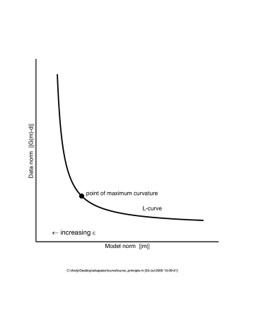
One way to gain insight into the problem is the L-curve (Hansen 1998, Farquharson & Oldenburg 2004), so called for its shape. To create this curve, the inversion is repeated for a range of regularization parameters and the data norm is plotted versus the model norm (figure 2) on a logarithmic scale. For large values of $\epsilon$ the model norm is small but the data norm is large. A small $\epsilon$ leads to a large model norm and to a data misfit norm that is close to the variance of the data. These two cases define the asymptotic behaviour of the L-curve. At the maximum curvature point of the curve, a compromise is found between the magnitude of those two norms (Hansen 1998). This is the optimal value for the regularization parameter.

Table 1: Parameters of the synthetic model used for the L-curve studies.

Parameter	Value	Unit
Sampling rate	20	m
Total depth of log	5000	m
Number of time steps for inversion	20
Start time of inversion	1000	ky b.p.
Stop time of inversion	0.1	ky b.p.

We studied our inversion problem with the help of the L-curve criterion. A synthetic temperature log was created using the parameter set given in table 1. The transient temperature anomaly given in figure 1 was added to the steady state solution and random, normally distributed noise was added. The noise amplitudes for the test data sets were 0.01, 0.2, 0.4, and 0.6 K, respectively.

Figure 3: L-Curve for different noise levels.

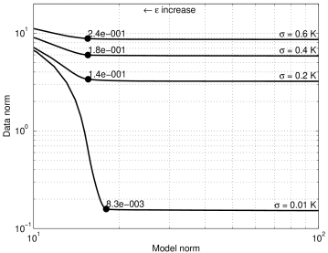
Figure 3 shows the variation of the L-curve and the optimum $\epsilon$ as a function of the noise level. It is apparent that only for the smallest noise level the L-curve takes on a well shaped form with an maximum curvature point easy to determine. For all noise levels the L-curve displays a straight line region where any change in $\epsilon$ leads to large changes in the model norm but does not change the data fit at all. This means that a value of $\epsilon$ less than the value found in the maximum curvature point is not justified by the data. It is noteworthy that the model norm of the optimal model does not vary much with the increasing noise level. This indicates that the inverted model is robust against noise for this configuration. This point is illustrated by comparing the inverted GST histories for optimal values of $\epsilon$ (figure 4).

Figure 4: Inverted GST-history for different noise levels and optimal $\epsilon$ from figure 3. The curves are each shifted by 5°C for better visibility.

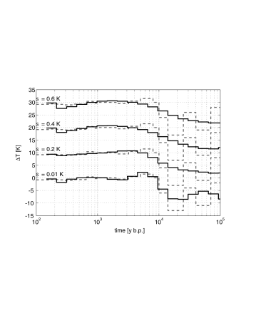
The major feature is the temperature increase at the end of the last ice age. It is preserved in all of the results in comparable magnitude and robust against noise. Smaller temperature variations during the Holocene period, on the other hand, are only resolved at the smallest noise level. The L-curve provides a tool to answer the important question if a sought for feature in the paleoclimate record can be resolved by the data.

Figure 5: GST-histories for a fixed noise level of 0.2 K and varying values of the damping parameter $\epsilon$. The optimal choice of $\epsilon$ according to the L-curve criterion is 0.14.

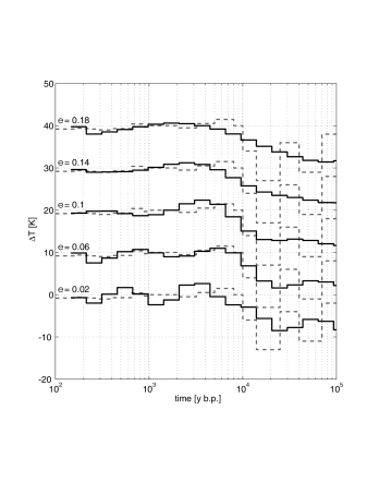
Finally, figure 5 shows a comparison of inversion results for a given noise level and a range of $\epsilon$-values. The optimal value would be about 0.14, yielding a rather smooth model. The interpreter, possibly aware of a paleoclimatic proxy curve like the ones shown in the figure, might be tempted to choose a smaller value that seems to better fit the temperature variations in the model during the Holocene. However, figure 3 indicates that the data fit does not improve at all by choosing an $\epsilon$ smaller than 0.14. The small amplitude variations on top of the temperature increase at the end of the ice age appear to be only numerical artifacts.

3 Sensitivity analysis

3.1 Length of the temperature log

Figure 6: A shortening of logs results in different GST reconstructions. Solid line represents the GSTH that was used to drive the forward model. The dashed lines show reconstructions for different depths of the logs. The temperature of the last glacial minimum is only resolved for the 3000 m log. Not even the timing of the climatic optimum in the Holocene is correctly resolved for the 1500 m log.

Table 2: Values for the thermal properties that are used throughout the text to compute synthetic temperature-depth profiles.

Parameter	Value	Unit
Thermal conductivity	$2.5$	W (m K)-1
Volumetric heat capacity	$2.30\cdot 10^{6}$	J m-3 K-1
Thermal diffusivity	$1.09\cdot 10^{-6}$	m2 s-1
Heat production rate	$1.0\cdot 10^{-6}$	W m-3
Surface temperature	$10.0$	°C
Heat flow	0.06	W m-2
Sampling rate	1.0	m

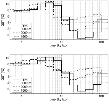
In the introduction the question was posed if the full depth range of the transient signal is needed for a valid reconstruction of the GST history. To analyze this problem, a synthetic temperature log with a simplified GST history of the last 1 million years is computed. The parameters for the temperature log are taken from table 2. The GST history that produces the transient temperature signal (grey line, figure 6) does not represent an actual paleoclimatic curve but rather represents an idealized history with correct order of magnitude for amplitude and timing of the events.

For the inversion procedure, the originally 3000 m deep log was cut off at depths of 2000 m and 1500 m. All three logs were inverted with and without synthetic noise applied. We chose normally distributed noise with a standard deviation of 0.3 K. For the inversion of the noise free and noisy logs, a constant damping parameter $\epsilon$ of 0.1 and 0.2, respectively, was used.

The resulting GST histories for the different inversion runs are displayed in figure 6. For both the noisy and the noise free data a log depth of 3000 m seems to be sufficient to fully recover the amplitude of the last glacial stage. A decrease of the maximum log depth also reduces the amplitude of the glacial cooling. Further the phase of the events is shifted to later times. The effect is more pronounced for the noisy data, but even for noise free data any reconstruction of the last ice age paleoclimate based on logs shallower than 2000 m seems to be problematic.

Figure 7: Upper panel: Various reconstructions of paleo temperatures of the last two millennia. Lower panel: Inversion results for a 2000 m deep noise free temperature log using the proxy-curve of Esper et al. (2002) as input data.

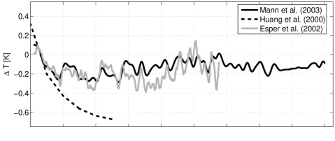
A similar procedure of shortening logs can be used to estimate the necessary depth of temperature logs for millennial scale climate reconstructions. Currently plenty of proxy reconstructions for the last one or two millennia exist and their validity is debated. The geothermal method can provide valuable insight into this problem as it is the only direct measurement of paleo-temperatures. The more it is important to analyze the information contained in the temperature data. Figure 7, upper panel, shows a few reconstructions of the Northern hemisphere annual mean SAT together with a reconstruction based on borehole temperature data (Mann & Jones 2003, Esper et al. 2002, Huang et al. 2000).

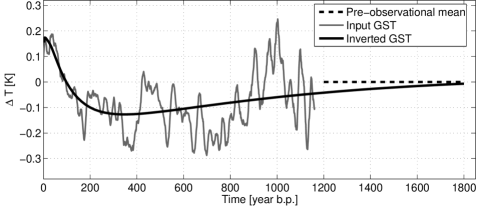
In our analysis we use the reconstruction of Esper et al. (2002) as the forcing to compute the transient temperature perturbation. The other parameters of the forward model are taken again from table 2. Additionally, a pre-observational mean needs to be specified. As the proxy curve contains no information about this parameter, it was arbitrarily chosen to be the mean temperature in the interval 800–1200 years before present. Figure 7, lower panel, displays an inversion result for this synthetic temperature log. The temperature data are noise free and the log runs 2000 m deep. Because of the favourable conditions for this particular inversion run the information contained in this reconstruction can be considered the maximum knowledge that can be extracted by inverting temperature-depth data. The warming trend of the last 200 years is captured very well. No insight into climate variations of the preceding centuries can be gained, but the pre-observational mean is preserved in the reconstruction. Thus the borehole method effectively provides two unknown pieces of information: The temperature change from the average temperature of the last millennium and the mean temperature before that period.

Figure 8: Inversion results for decreasing maximum depth of the temperature log. Temperature logs were cut off at various depths. Thermal parameters are the same as in table 2. Upper panel: Input temperature data for the inversion was noise-free. The damping parameter $\epsilon$ equals 0.1. Lower panel: Temperature data are disturbed by normally distributed noise with a standard deviation of $\sigma=0.1$ K. A higher $\epsilon$ of 0.6 is used in the inversion.

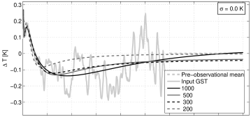
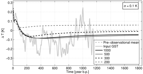
These considerations are only valid for the best available data. In reality, data are noisy and boreholes are not sufficiently deep to allow extraction of this information from the temperature data. Figure 8 compares inversion results where only shorter logs are available and noise is added to the data. For the case without noise, the average temperature of the last millennium can be resolved for logs that run deeper than 300 to 500 m. For shallower logs a strong decrease in amplitude of the GST reconstruction is apparent. If noise is present in the data even the 1000 m temperature is not able to fully recover the mean temperature of the last 1000 years. These observations are different from the results for glacial/post-glacial reconstructions. The reason is that the amplitude of the transient temperature signal due to temperature changes in the last few thousand years is one order of magnitude less than that observed for the post-ice age temperature rise (see figure 1). The input signal used here is a global SAT reconstruction. At a specific site the amplitude of the transient signal can be higher and thus improve the signal to noise ratio that we assume in our example. Thus, in practice the expected signal should be compared to the noise present in the data to assess if the desired signal can be extracted from the data.

Figure 9: Estimating the transient temperature anomaly and undisturbed gradient results in a biased estimate for the gradient and a smaller temperature anomaly.

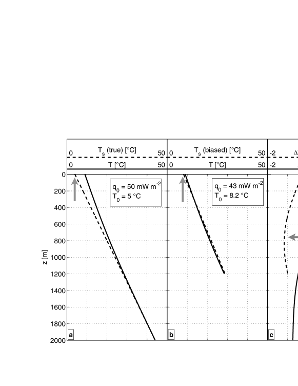
Both examples show a strong dependence of the inverted GST history on data quality and both fail to reproduce the input forcing under certain circumstances. The ill-posed nature of the problem together with the regularization using the damping parameter $\epsilon$ cause this behaviour. Besides preventing numerical instability in the inversion the procedure also minimizes the norm of the parameter vector. Usually this effect is desired to avoid unnecessary complicated models (Constable et al. 1987). However, in our case a minimal solution in this sense will have smaller GST variations compared to the GST variations that created the transient temperature anomaly. This is especially true since the mean GST $T_{0}$ and the surface heat flow $q_{0}$ are also solved for. Figure 9 illustrates this problem. The black line denotes the true temperature perturbation due to a step increase in ground surface temperature. If one inverts simultaneously for GST history, $q_{0}$, and $T_{0}$ using a minimum norm model in the presence of noise, a steady state temperature profile (grey line) tilted toward the temperature anomaly will be obtained instead the true one (dashed black line). In a case with a step increase in GST, the estimate for $q_{0}$ will be too low and that for $T_{0}$ will be too high. An example of this trend will be given in the case example. It is also notable that the temperature perturbation crosses the steady-state profile at two points (arrows). Thus, a false GST history is created with a decrease in ground surface temperature and a subsequent increase although the input model uses only a step increase. Even with an $\epsilon$ chosen optimal for the inversion, this problem will persist as it is imminent in the regularization.

3.2 Thermal parameters

Figure 10: Systematic changes in thermal diffusivity cause shifts in the timing of the events. Thermal conductivity is varied from 70 % to 130 % of the original value. For better visibility, inverted curves are stacked and plotted as smooth lines rather than a series of step functions.

Figure 11: Systematic changes in heat production rate cause variations in the amplitude of the events. Heat production rate is varied from 70 % to 130 % of the original value. The inverted curves are plotted as smooth lines rather than a series of step functions for better visibility of the effect.

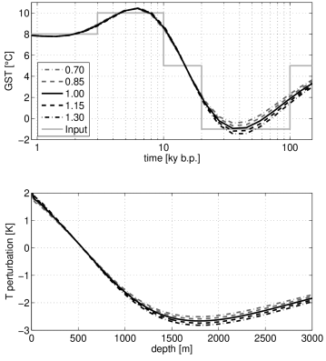
The inversion procedure requires that thermal conductivity, thermal diffusivity, and heat production rate are exactly known. In a real situation errors for this parameters can be minimized but cannot be avoided altogether. For instance errors might be introduced by preferential sampling of units that are not representative of the whole sequence. Also, missing or false corrections for in-situ conditions of temperature and pressure can cause systematic deviations from the correct thermal parameters. In the following the uncertainties in the inversion resulting from these errors are considered.

In general, the inversion procedure interprets curvature in the temperature log as a transient signal. Thus, only the terms introducing curvature in equation 1 will have an influence on the inversion result. The transient term of the model has thermal diffusivity as its only relevant parameter. We can expect that this property will have the largest influence on the solution. Within the steady state terms, only the heat production term introduces curvature. As heat production rate is usually small, the influence of this term is expected to be less important for boreholes of moderate depth (see 3.2). Heat production and thermal conductivity are related inverse proportional in this term. Thus, to analyze the errors introduced by this term, only on of the parameters needs to be studied. We chose the heat production rate. Thermal conductivity has its main influence in the steady-state terms for heat conduction. A false assumption will therefore lead directly to a proportional error in the heat flow density but does not affect the transient part of the temperature log. In practice, of course, thermal diffusivity is indirectly determined as the ratio of thermal conductivity and volumetric heat capacity and will have an indirect effect on the solution.

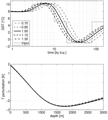
In order to support this qualitative discussion with quantitative results a synthetic temperature log was inverted with false assumptions of thermal diffusivity and heat production rate in two separate inversion runs. The parameters were varied by $\pm$30% of the original value. A simplified GST history was used in the forward model to compute the transient temperature anomaly. The GST history used is comprised of several step changes that aim to reproduce the general magnitude and timing of the expected effects and do not represent an actual GST history. The results of these experiments are shown in figures 10 and 11. Thermal diffusivity influences the timing of events in the reconstructed time series. A phase shift of the entire reconstruction occurs when a false estimate is used in the inversion. The amplitude of computed past temperature remains unchanged. Heat production influences the magnitude of the paleoclimatic events but retains timing of events. The effect of the heat production increases with time, consistent with the fact that the heat production term increases quadratically with depth. It is apparent, that the heat production will only be significant for very large deviations from the correct value and deep boreholes. For instance, it should be irrelevant for millennial scale studies. Thermal diffusivity can change the timing of events on all timescales and it is also important for inversions of much shorter timescales than considered here.

3.3 Heterogeneity

The previous discussion considered a homogeneous subsurface only. The question is of course whether the conclusions drawn a valid for a heterogeneous medium. To address this question we will assess the impact of a heterogeneous 1D layered earth model on the results of the inversion. In the following the transient profiles computed by a FD algorithm (Rath & Mottaghy 2005) will be considered as ground truth. Random variations of the thermal properties on distinct length scales will be introduced and the inversion results studied. We will discuss the effect of systematic variations on a synthetic example of a sedimentary rock column. We will study the steady state $T$-$z$ profile that results from compaction and elevated temperatures.

For the forward computation a simplified GST history of the last 100 000 years is used, with a pre-observational mean of 5°C. The profile is computed down to 10 000 m with a vertical resolution of 5m. For the analysis only the top 3000 m are used, the deeper parts are only necessary to avoid edge effects in the solution. Thermal parameters are those of table 2 if not explicitly specified.

Obviously, the largest influence on the temperature profile will come from variations in thermal conductivity. Deviations from the straight line that is assumed for the stationary temperature will be falsely interpreted as noise or paleoclimate. In the homogeneous subsurface framework it is impossible to study variations of $\lambda$ and $\kappa$ separately. One way to overcome this problem is to cast the steady state part of the equation in terms of the Bullard depth $z_{b}$, for the homogeneous case defined by $z_{b}=z/\lambda$. Consider the differential equation for 1D heat transport in a homogeneous medium:

$$\frac{\partial^{2}T}{\partial z^{2}}=\frac{1}{\kappa}\frac{\partial T}{\partial t}+\frac{A}{\lambda}.$$ (5)

Substituting $\partial z=\lambda\partial z_{b}$ yields

$$\frac{\partial^{2}T}{\lambda^{2}\partial z_{b}^{2}} = \frac{1}{\kappa}\frac{\partial T}{\partial t}+\frac{A}{\lambda}$$ (6)

$$\Rightarrow\frac{\partial^{2}T}{\partial z_{b}^{2}} = \frac{\lambda^{2}}{\kappa}\frac{\partial T}{\partial t}+\lambda A$$ (7)

Thus if $\kappa^{\prime}=\kappa/\lambda^{2}$ and $A^{\prime}=A/\lambda^{2}$, equation 1 can be written as:

$$T(z_{b}) = T_{0}+q_{0}z_{b}+\frac{A^{\prime}z_{b}^{2}}{2}$$ (8)

$$+ \sum\limits_{j=1}^{N}T_{n}^{G}\left(\mbox{erfc}\left(\frac{z}{2\sqrt{\kappa}^{\prime}t_{j}}\right)-\mbox{erfc}\left(\frac{z}{2\sqrt{\kappa}^{\prime}t_{j-1}}\right)\right)$$

Using the transformed variables and taking the heat production term to the left hand side, the steady state part of the profile can be reduced to a homogeneous problem. With this construct it is possible to use a layered model for the thermal conductivity and a homogeneous one for the thermal diffusivity. This allows us to study the influence of thermal diffusivity alone in the algorithm. With the general framework established, we will now turn to the different aspects of heterogeneity.

Figure 12: Misfit between temperature profiles computed from the FD-model and homogeneous models for varying length scales of variability. Mean RMS-values are given for a homogeneous subsurface ($\diamond$) and for homogeneous $\kappa$ only ($\circ$). Grey areas denote min/max range.

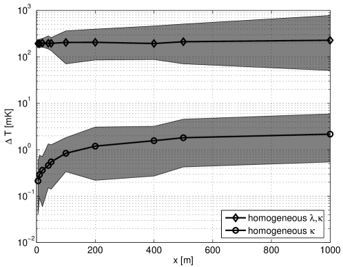
The noise on varying length scales has been studied by modifying the FD model to compute the temperature profiles. The layers of the model were assigned random values of thermal conductivity with a mean of 2.5 W(m K)-1 and a standard deviation of 0.5 W(m K)-1. Volumetric heat capacity was held constant throughout the experiment, resulting in a simultaneous variation of thermal conductivity and diffusivity. Ten different configurations were considered with layer widths $x$ increasing from 5 m to 1000 m. For each configuration 50 realizations of the thermal conductivity-depth profile were generated. These were then used in the forward model to compute 50 temperature depth profiles. Additionally, temperature profile for an equivalent half space and for a layered representation (equation 8) were computed. The differences between the “true” temperature profile and the two profiles with assumptions are shown in figure 12. The misfit of the equivalent homogeneous model is large because variations in the steady state temperature profile are not reflected in the homogeneous model. This highlights the importance of the knowledge of thermal conductivity. On the other hand, for the model with homogeneous $\kappa$ only deviations of the order of a few mK occur, suggesting that random variations of thermal diffusivity are smoothed out.

Figure 13: Variation of the timing and amplitude of the maximum temperature in the Holocene versus the length scale of the random noise as defined in the text. Left: Value of the maximum temperature. Right: Timing of the maximum value. Grey area denotes 75 % quartiles of all realizations.

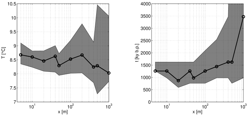
Next, the random data have been used as input to the inversion procedure. For each inversion the value and timing of the maximum temperature in the Holocene have been recorded in order to compress the results (figure 13). To accommodate the increasing misfit between model and data for increasing noise length scale, the damping parameter $\epsilon$ was increased from 0.35 to 1 according to an increase in noise length scale from 5 m to 1000 m. This leads to a stronger damping and is reflected in the decrease of the maximum temperature value because models with smaller norms are preferred for large $\epsilon$. The influence of noise on the result becomes most pronounced for length scales larger than 100 m when the scale of the signal is on the order of the noise scale. The timing of the event is modified in a similar way.

Figure 14: Systematic variation of thermal properties with depth. a) Porosity, temperature, and reduced temperature; b) thermal conductivity and heat capacity of the rock matrix, depending on temperature; c) effective thermal conductivity and diffusivity with porosities from panel a); d) Effective thermal properties for constant porosity of 0.1.

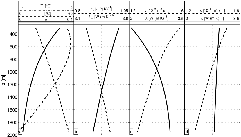
In crystalline rocks random variations of thermal properties might prevail, in sedimentary rocks systematic changes are much more important. Changing depositional environments throughout time create diverse rock types. The influence on the inversion depends on the particular setting. One aspect that is often neglected is the variation of thermal properties in uniform sequences of rock due to the temperature dependence of thermal properties and the compaction with increased overburden. In figure 14 a geologic profile of a single rock type is considered. The thermal conductivity of the matrix is taken as 3.5 W(m K)-1. An exponential decrease of porosity due to compaction is assumed (Athy’s law) with a surface porosity of 0.45 and a characteristic depth of 750 m (Allen & Allen 1990). Thermal conductivity of the matrix is taken inversely proportional to temperature (Haenel et al. 1988) and heat capacity of the matrix is approximately proportional to temperature in the range considered. For simplicity the pore fluid is assumed to be fresh water, thermal properties are taken from reference tables (Wagner & Pruß 2002, Kaye & Laby 1968). Temperature and heat flow at the surface are 10 °C and 0.06 W m-2, respectively. These assumptions lead to a curvature in the thermal properties (figure 14 c). The curvature is reflected in the reduced temperature $T_{r}$ (figure 14 a). This effect is similar in magnitude to the influence of paleoclimate. It is apparent that these effects need to be taken into account for any paleoclimate inversion.

For comparison, effective thermal rock properties are also given for a constant porosity of 0.1 to consider only the temperature/pressure effects (figure 14 d). The shape of the $\lambda-z$ profile changes considerably displaying the prominent influence of the porosity decrease. The $\kappa-z$ profiles show that the porosity effect is compensating the temperature effect. Diffusivity varies by about 20 % in this example. When comparing these results to the inversions of the previous sections it is clear that thermal conductivity needs to be known accurately to achieve reliable results. Diffusivity is again somewhat less important.

4 Case study: KTB

Figure 15: Composite log, KTB pilot hole. Panels from left to right: 1) Spectral Gamma Ray (SGR), temperature (TEMP), temperature gradient (TMPG); 2) Generalized lithology; 3) Thermal conductivity: Core measurements (TC), mean value (mean TC), $\pm 1\sigma$ of the mean value (shaded area), corrected for temperature and pressure (corr TC); 4) Heat production $A$ from spectral gamma ray (A), mean value of $A$ (mean A), thermal diffusivity $\kappa$ (TD).

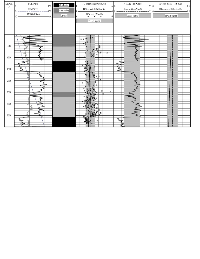
A temperature log assumed to be in equilibrium was recorded in the KTB pilot hole down to 3990 m on September 17, 1997 and analyzed in Clauser (1999). An earlier recording, dating from February 1996, was analyzed in detail for thermal processes, including transient effects of paleoclimate (Clauser et al. 1997). Shallow temperature logs in the vicinity of the KTB site have also been interpreted in terms of paleoclimatic influence (Clauser & Mareschal 1995, Clauser 1999). In the light of the previous sections, we will revisit the analysis of the KTB borehole and discuss the uncertainties connected with the interpretation. In that study the temperature data was inverted for paleoclimate in the period from 105 to 102 years before present, using 100 time steps, a thermal conductivity of 2.92 W (m K)-1, a thermal diffusivity of 10-6 m2 s-1, and a heat production rate of 1.1 $\mu$W m-3. Their analysis yielded a peak to peak amplitude of 10 K for the temperature increase from the latest glacial stage to the Holocene.

The geological profile in the KTB pilot hole is primarily composed from two lithologies: Metabasites and Gneisses. These can easily be separated using the Gamma-ray-log (SGR) (figure 15, left panel). Thermal conductivity (figure 15, right panel) does not seem to vary systematically over the depth of the borehole, justifying the assumption of a homogeneous half-space. The mean thermal conductivity is $(2.93\pm 0.60)$ W(m K)-1. This value reduces to 2.82 W(m K)-1 if a temperature-pressure correction is applied to the data (Buntebarth 1991). Knowledge of the thermal diffusivity is much more uncertain. Literature cites ranges for Gneisses and Amphibolites as 0.5 to 1.2$\cdot 10^{-6}$ m2 s-1 and 0.6 to 0.8$\cdot 10^{-6}$ m2 s-1, respectively (Landolt-Börnstein 1982). Seipold (1995) reports $(0.8\pm 0.2)\cdot 10^{-6}$ m2 s-1 for Amphibolite samples from neighbouring sites. Again, a correction for temperature and pressure of the value given by Seipold (1995) reduces the mean diffusivity to a value of 0.70 m2 s-1.

Figure 16: L-curve for the inversion of the KTB pilot hole-temperature log.

Figure 17: Inverted GST histories for varying values of the damping parameter.

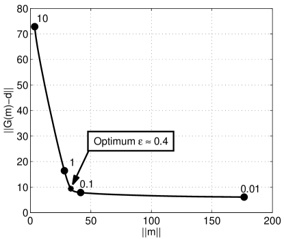
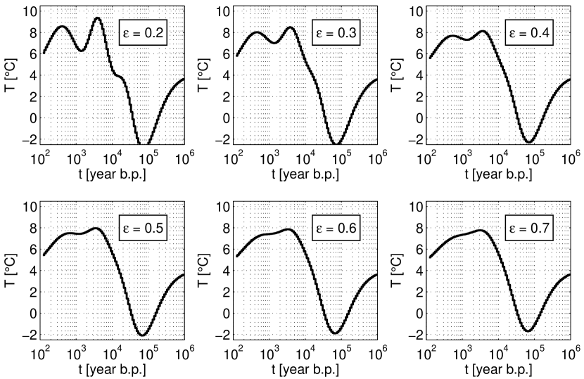
The next step in the analysis is the choice of the optimum regularization parameter $\epsilon$. Figure 16 shows the L-curve for varying values of $\epsilon$. The optimum choice seems to be $\epsilon=0.4$. Figure 17 highlights this in more detail. The inverted time series for the different values of $\epsilon$ are shown. The direct comparison of results is especially helpful to analyze which features of the GST history are numerical oscillations and which ones represent actual information. At a level of 0.4 oscillations that change the warming amplitude seem to be dampened out. A more conservative interpreter might choose an even higher value of 0.6, but in this range of $\epsilon$-values the main features are only changed by a few tenth of a degree Celsius.

Figure 18: Inversion results for the KTB log for different depths of the log. Top: Inverted GST history for different log length. For clarity, the step amplitudes of the GST histories are shown as continuous lines. Bottom: Transient temperature signal in the subsurface.

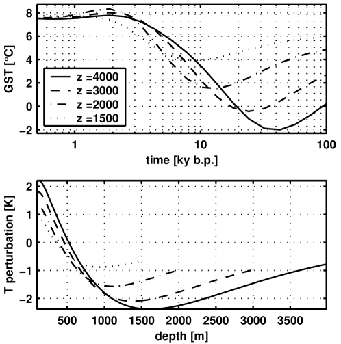
Following the choice of the damping parameter, we shortened the log to illustrate the detrimental effect of the log length. The maximum depth of originally 3990 m was successively cut to lengths of 3000, 2000, and 1500 m. Figure 18 shows the reconstructed GSTH and transient temperature perturbation in the borehole for various cut off depths. Deviations from the expected results become significant for depths less than 2500 m. It is noteworthy that not only the temperature drop of the last glacial stage decreases but also the timing of the optimum temperature in the Holocene changes. An interpreter of paleoclimatic inversions must be aware that the post glacial temperature increase will influence the shape and timing of later events as well.

Table 3: Inversion results for the KTB log, cut off at various depths. The inverted parameters vary systematically with the depth of the log.

Depth (m)	$T_{0}$ (°C)	$q$ (mW m-2)	$dT/dz$ (mK m-1)
4000	4.14	86.3	29.6
3000	4.70	84.8	29.6
2000	5.51	81.8	28.0
1500	6.15	78.1	26.7

Table 3 shows the inversion results for the undisturbed GST (i. e. the pre-observational mean), the heat flow into the model and the undisturbed gradient. This highlights that the systematic variation of the GST history is accompanied by an according change in the steady-state parameters. As discussed in the section on length of temperature logs, the heat flow value decreases whereas the GST increases. This is consistent with inverting a step increase in ground surface temperature using a log that is too short too fully resolve the GST history. It can be expected from this data that crustal heat flow estimates may be too low by about 8 mW m-2, if a transient signal of the last ice age has not been properly removed.

5 Conclusions

The sensitivity analyzes in the previous sections have shown that the inversion results are strongly dependent on data quality. The parameters most important depend on the time scale of inversion. For inferences about the post-glacial temperature rise the maximum depth of the temperature log is the most challenging requirement. If it is met, the inversion is robust against noise in the temperature data. A depth of more than 3000 m seems to be optimal to resolve the temperature rise adequately. Unfortunately, undisturbed temperature logs running that deep are rare. Reconstructions of the last millennium require only modestly deep logs. A depth of about 300 m to 500 m is suitable to derive a mean temperature for the last 1000 years. The exact values will depend on the magnitude of the noise and the transient signal at a specific site. For instance the IHFC database for borehole temperatures and climate reconstruction lists 473 out of 754 temperature logs with a maximum depth greater than 300 m (http://www.geo.lsa.umich.edu/~climate). However, for this type of inversion the demand on data fidelity is very high. Even a noise level of 0.1 K seriously degrades the inversion results. In practice the noise level a

Errors in the thermal properties, namely thermal diffusivity and heat production, seem not to be the main source of error. The diffusive nature of the signal and the spreading over a wide depth range greatly dampen the influence of the thermal diffusivity. The importance of heat production increases with reconstruction length. But even for studies of the last 100 000 years errors introduced by false assumptions of the heat production rate will be small compared to other sources of error.

The studies on the regularization parameter show that a thorough noise analysis should accompany any attempt to invert GST histories from geothermal data. The correct choice of the regularization is crucial and should be justified by some objective means. A non-optimal choice of the regularization can easily lead to artefacts that are much larger than the calculated model errors. Especially to small an $\epsilon$ introduces events that could be mistaken for variations of paleo-temperatures. We used the L-curve criterion but other methods like generalized cross validation (e. g.,  Hansen 1998, Haber & Oldenburg 2000, Aster et al. 2004) or truncated iterative methods (e. g.,  Hansen 1998, Hanke 1995, Berglund 2002)could also be utilized.

Finally, although the least-squares fit with a Tikhonov regularization minimizing the model norm is a generally applied method in solving ill-posed problems, it might not necessarily be the best choice, as pointed out by Hansen (1998). Other regularization methods might better preserve the information contained in borehole temperatures. These include Bayesian-type smoothing approaches (Serban & Jacobsen 2001) as well as nonlinear minimum support regularizers (Portniaguine & Zhdanov 1999, Zhdanov 2002, Zhdanov & Tolstaya 2004). Research in the development of novel approaches to regularization and the incorporation of prior knowledge are an urgent task for the future.

References

- (1)
- Allen & Allen (1990) Allen, P. A. & Allen, J. R. (1990), Basin Analysis. Principles and Applications, Blackwell Scientific, Oxford.
- Aster et al. (2004) Aster, R., Borchers, B. & Thurber, C. (2004), Parameter estimation and inverse problems, Academic Press, San Diego.
- Beck et al. (1992) Beck, A. E., Shen, P. Y., Beltrami, H., Mareschal, J.-C., Šafanda, J., Sebagenzi, M. N., Vasseur, G. & Wang, K. (1992), A comparison of five different analyses in the interpretation of five borehole temperature data sets, in Lewis (1992), pp. 101–112.
- Beltrami & Bourlon (2004) Beltrami, H. & Bourlon, E. (2004), ‘Ground warming patterns in the Northern Hemisphere during the last five centuries’, Global and Planetary Change 227(3-4), 169–177.
- Beltrami et al. (1995) Beltrami, H., Chapman, D. S., Archambault, S. & Bergeron, Y. (1995), ‘Reconstruction of high resolution ground temperature histories combining dendrochronological and geothermal data’, Earth and Planetary Science Letters 136(3-4), 437–445.
- Beltrami et al. (1997) Beltrami, H., Cheng, L. & Mareschal, J. C. (1997), ‘Simultaneous inversion of borehole temperature data for determination of ground surface temperature history’, Geophysical Journal International 129, 311–318.
- Beltrami & Mareschal (1995) Beltrami, H. & Mareschal, J.-C. (1995), ‘Resolution of ground temperature histories inverted from borehole temperature data’, Global and Planetary Change 11(1–2), 57–70.
- Beltrami & Taylor (1995) Beltrami, H. & Taylor, A. E. (1995), ‘Records of climatic change in the canadian arctic: Towards calibrating oxygen isotope data with geothermal data’, Global and Planetary Change 11(3), 127–138.
- Berglund (2002) Berglund, A.-C. (2002), Nonlinear Regularization -with Applications to Geophysics, PhD thesis, Department of Informatics and Mathematical Modeling, Technical University of Denmark.
- Buntebarth (1991) Buntebarth, G. (1991), ‘Thermal properties of KTB-Oberpfalz VB core samples at elevated temperature and pressure’, Scientific Drilling 2, 73–80.
- Carslaw & Jaeger (1959) Carslaw, H. S. & Jaeger, J. C. (1959), Conduction of heat in solids, 2nd edn, Oxford University Press.
- Clauser (1999) Clauser, C. (1999), Thermal signatures of heat transfer processes in the Earth’s crust, Springer, Berlin–Heidelberg.
- Clauser et al. (1997) Clauser, C., Giese, P., Huenges, E., Kohl, T., Lehmann, H., Rybach, L., Šafanda, J., Wilhelm, H., Windloff, K. & Zoth, G. (1997), ‘The thermal regime of the crystalline continental crust: Implications from the KTB’, Journal of Geophysical Research 102(B8), 18417–18441.
- Clauser & Mareschal (1995) Clauser, C. & Mareschal, J. C. (1995), ‘Ground temperature history in central Europe from borehole temperature data’, Geophysical Journal International 121(3), 805–817.
- Constable et al. (1987) Constable, S. C., Parker, R. L. & Constable, C. G. (1987), ‘Occam’s inversion: A practical algorithm for generatlng smooth models from electromagnetic sounding data’, Geophysics 52(3), 289–300.
- Esper et al. (2002) Esper, J., Cook, E. R. & Schweingruber, F. H. (2002), ‘Low-frequency signals in long tree-ring chronologies for reconstructing past temperature variability’, Science 295, 2250–2253.
- Farquharson & Oldenburg (2004) Farquharson, C. G. & Oldenburg, D. W. (2004), ‘A comparison of automatic techniques for estimating the regularization parameter in non-linear inverse problems’, Geophysical Journal International 156, 411–425.
- González-Rouco et al. (2003) González-Rouco, F., von Storch, H. & Zorita, E. (2003), ‘Deep soil temperature as proxy for surface air-temperature in a coupled model simulation of the last thousand years’, Geophysical Research Letters 30(21), 2116, doi:10.1029/2003GL018264.
- Haber & Oldenburg (2000) Haber, E. & Oldenburg, D. (2000), ‘A GCV based method for nonlinear ill-posed problems’, Computational Geosciences 4(1), 41–63.
- Haenel et al. (1988) Haenel, R., Rybach, L. & Stegena, L., eds (1988), Handbook of terrestrial Heat-Flow Density Determination, Solid Earth Science Library, Kluwer Academic Publishers.
- Hanke (1995) Hanke, M. (1995), Conjugate Gradient Type Methods for Ill-posed Problems, Pitman Research Notes in Mathematics, Longman Scientific and Technical, Harlow, UK.
- Hansen (1998) Hansen, P. C. (1998), Rank Defficient and discrete ill-posed Problems. Numerical Aspects of Linear Inversion, SIAM, Philadelphia.
- Huang et al. (2000) Huang, S., Pollack, H. N. & Shen, P.-Y. (2000), ‘Temperature trends over the past five centuries reconstructed from borehole temperatures’, Nature 403, 756–758.
- Jones et al. (1999) Jones, M., Tyson, P. & Cooper, G. (1999), ‘Modelling climatic change in South Africa from perturbed borehole temperature profiles’, Quarternary International 57/58, 185–192.
- Kaye & Laby (1968) Kaye, G. W. & Laby, T. H. (1968), Tables of Physical and Chemical Constants, Longmans, London.
- Kohl (1998) Kohl, T. (1998), ‘Palaeoclimatic temperature signals — can they be washed out?’, Tectonophysics 291, 225–234.
- Kohl (1999) Kohl, T. (1999), ‘Transient thermal effects below complex topographies’, Tectonophysics 306, 311–324.
- Lanczos (1961) Lanczos, C. (1961), Linear Differential Operators, Van Nostrand, London.
- Landolt-Börnstein (1982) Landolt-Börnstein (1982), Physical Properties of Rocks, Vol. V, Springer.
- Lewis (1992) Lewis, T. J., ed. (1992), Climatic Change Inferred from Underground Temperatures, Vol. 98 of Paleogeography, Paleoclimatology, Paleoecology (Global and Planetary Change Section), Elsevier, Amsterdam.
- Mann & Jones (2003) Mann, M. E. & Jones, P. D. (2003), ‘Global surface temperatures over the past two millennia’, Geophysical Research Letters 30(15), 1820, doi:10.1029/2003GL017814.
- Mann & Schmidt (2003) Mann, M. E. & Schmidt, G. A. (2003), ‘Ground vs. surface air temperature trends: Implications for borehole surface temperature reconstructions’, Geophysical Research Letters 30(12), 1607, doi:10.1029/2003GL017170.
- Mareschal & Beltrami (1992) Mareschal, J.-C. & Beltrami, H. (1992), ‘Evidence for recent warming from perturbed geothermal gradients: Examples from Eastern Canada’, Climate Dynamics 6, 135–143.
- Menke (1989) Menke, W. (1989), Geophysical Data Analysis: Discrete Inverse Theory, number 45 in ‘International Geophysics Series’, rev. edn, Academic Press.
- Nitoiu & Beltrami (2005) Nitoiu, D. & Beltrami, H. (2005), ‘Subsurface thermal effects of land-use changes’, Journal of Geophysical Research 110, F01005, doi:10.1029/2004JF000151.
- Portniaguine & Zhdanov (1999) Portniaguine, O. & Zhdanov, M. S. (1999), ‘Focusing geophysical inversion images’, Geophysics 64, 874–887.
- Rath & Mottaghy (2005) Rath, V. & Mottaghy, D. (2005), ‘Joint inversion for ground surface temperature histories: a case study from the Kola Peninsula, Russia’, Geophysical Journal International Submitted.
- Reiter (2005) Reiter, M. (2005), ‘Possible ambiguities in subsurface temperature logs: Consideration of ground-water flow and ground surface temperature change’, Pure and Applied Geophysics 162, 343–355.
- Seipold (1995) Seipold, U. (1995), ‘The variation of thermal transport properties in the Earth’s crust’, Journal of Geodynamics 20(2), 145–154.
- Serban & Jacobsen (2001) Serban, D. Z. & Jacobsen, B. H. (2001), ‘The use of broad-band prior covariance for inverse paleoclimate estimation’, Geophysical Journal International .
- Shen & Beck (1991) Shen, P. Y. & Beck, A. E. (1991), ‘Least squares inversion of borehole temperature measurements in functional space’, Journal of Geophysical Research 96(B12), 19965–19979.
- Shen & Beck (1992) Shen, P. Y. & Beck, A. E. (1992), Paleoclimate change and heat flow density inferred from temperature data in the Superior Province of the Canadian Shield, in Lewis (1992), pp. 143–165.
- Shen et al. (1995) Shen, P. Y., Pollack, H. N., Huang, S. & Wang, K. (1995), ‘Effects of subsurface heterogeneity on the inference of climate change from borehole temperature data: Model studies and field examples from Canada’, Journal of Geophysical Research 100(B4), 6383–6396.
- Signorelli & Kohl (2004) Signorelli, S. & Kohl, T. (2004), ‘Regional ground surface temperature mapping from meteorological data’, Global and Planetary Change 40, 267–284.
- Taniguchi et al. (1999) Taniguchi, M., Shimada, J., Tanaka, T., Kayane, I., Sakura, Y., Shimano, Y., Dapaah-Siakwan, S. & Kawashima, S. (1999), ‘Disturbances of temperature-depth profiles due to surface climate change and subsurface water flow: 1. An effect of linear increase in surface temperature caused by global warming and urbanization in the Tokyo metropolitan area, Japan’, Water Resources Research 35(5), 1507–1517.
- Wagner & Pruß (2002) Wagner, W. & Pruß, A. (2002), ‘The IAPWS formulation 1995 for the thermodyamic properties of ordinary water substance for general and scientific use’, Journal of Physical and Chemical Reference Data 31, 387–535.
- Zhdanov (2002) Zhdanov, M. S. (2002), Geophysical inverse theory and regularization problems, Elsevier, Amsterdam.
- Zhdanov & Tolstaya (2004) Zhdanov, M. S. & Tolstaya, E. (2004), ‘Minimum support nonlinear parametrization in the solution of a 3D magnetotelluric inverse problem’, Inverse Problems 20(3), doi:10.1088/02665611/20/3/017.