Impact of Point Source Clustering on Cosmological Parameters with CMB Anisotropies

Abstract

The faint radio point sources that are unresolved in cosmic microwave background (CMB) anisotropy maps are likely to be a biased tracer of the large-scale structure dark matter distribution. While the shot-noise contribution to the angular power spectrum of unresolved radio point sources is included either when optimally constructing the CMB angular power spectrum, as with WMAP data, or when extracting cosmological parameters, we suggest that clustering part of the point source power spectrum should also be included. This is especially necessary at high frequencies above 150 GHz, where the clustering of far-IR sources is expected to dominate the shot-noise level of the angular power spectrum at tens of arcminute angular scales of both radio and sub-mm sources. We make an estimate of source clustering of unresolved radio sources in both WMAP and ACBAR, and marginalize over the amplitude of source clustering in each CMB data set when model fitting for cosmological parameters. For the combination of WMAP 5-year data and ACBAR, we find that the spectral index changes from the value of $0.963\pm 0.014$ to $0.959\pm 0.014$ (at $68\%$ c.l.) when the clustering power spectrum of point sources is included in model fits. While we find that the differences are marginal with and without source clustering in current data, it may be necessary to account for source clustering with future datasets such as Planck, especially to properly model fit anisotropies at arcminute angular scales. If clustering is not accounted and point sources are modeled with a shot-noise only out to $l\sim 2000$, the spectral index will be biased by about 1.5$\sigma$.

I Introduction

As discussed in a variety of papers, unresolved radio point sources are an important foreground in temperature anisotropy maps of the cosmic microwave background (CMB) zotti ; tof1 ; wright ; tegmark . With Wilkinson Microwave Anisotropy Probe (WMAP) data bennett , the difference in the CMB power spectra determined at various frequency channels and the cross power spectra between the channels, has allowed the unresolved point source contamination to be constrained with an amplitude $A_{\rm ps}=(0.011\pm 0.001)\mu$K²-sr nolta for the foreground power spectrum, when scaled to the Q-band. In the WMAP analysis, this point source amplitude is taken to be a constant in $C_{l}$, similar to the case of a shot-noise type power spectrum for unresolved point sources. This shot-noise, with an appropriate scaling in frequency, is then removed from each of the power spectra when constructing the final WMAP temperature anisotropy power spectrum hinshaw .

While the WMAP estimate on the point source correction is consistent with a point source power spectrum dominated by the shot-noise, this estimate is dominated by measurements relative to the Q-band nolta . Since the WMAP temperature anisotropy power spectrum is based on V- and W-band data dunkley , and the point source correction has a larger uncertainty in V- and W- bands nolta , it is unclear if a simple shot-noise correction fully describes point sources in the WMAP temperature anisotropy power spectrum. To account for uncertainty in the amplitude of point-source shot-noise in parameter estimates, the WMAP likelihood contains an additional marginalization of the uncertainty of $A_{\rm ps}$, but the best-fit amplitude of point-sources remain fixed to the a priori determined value hinshaw . We also note that alternative approaches have been considered to estimate the amplitude of point-sources Huffenberger1 ; Huffenberger2 , though these works also concentrated on establishing the shot-noise correction.

Beyond the shot-noise, unresolved radio point sources are likely to have a clustered distribution on the sky as they are expected to be a biased tracer of the large-scale structure. Thus, the angular power spectrum of sources contains not just a shot-noise but also a clustering piece determined by the dark matter power spectrum, point source bias, and the redshift distribution. Existing calculations suggest that the shot-noise part of the power spectrum from bright, rare sources dominates clustering at low radio frequencies, especially when the flux threshold for point source removal is at the level of $\sim$ 1 Jy GonzalezNuevo:2004fj ; tof1 . Thus, the assumption of a shot-noise point source contribution to the angular power spectrum of temperature anisotropies is likely to be adequate for low-frequency bands of WMAP such as the Q-band, but may not be appropriate at high frequencies, such as the W band, whose data are used in the temperature power spectrum.

The approach using a shot-noise spectrum with an uncertainty that is marginalized over in the WMAP likelihood is is bit different from the approach advocated by the WMAP team to account for another foreground in CMB data involving the Sunyaev-Zel’dovich (SZ) effect from galaxy clusters. There, the angular power spectrum is estimated based on a model for the cluster distribution and gas properties Komatsu , with an overall uncertainty in the amplitude of the SZ power spectrum captured by a free parameter which is then freely varied as a nuisance parameter when best-fit cosmological parameter values and their uncertainties using a Markov-Chain Monte-Carlo (MCMC) code lewis ; spergel ; dunkley .

Since the clustering component of the angular power spectrum of unresolved radio sources may be important, it could be that simply including point-sources as a shot-noise correction in the V/W-band WMAP temperature anisotropy power spectrum results in biased estimates of cosmological parameters, especially for parameters like the spectral index of density perturbations, which has been discussed previously in the context of uncertainties related to point-source shot-noise amplitude Huffenberger1 . Moreover, current CMB analyses make use of the combination of datasets such as WMAP and ACBAR which have different treatments related to how point sources are accounted in the parameter fits. At the ACBAR frequency of 150 GHz reichardt , the clustering of sources may need to be included properly, especially given that the high angular resolution of ACBAR also allows removal of sources down to a lower flux density level, where the shot-noise associated with rare, bright sources may be subdominant. The clustering of point sources could also account for some fraction of the excess arcminute-scale anisotropies detected by ACBAR tof2 ; Cooray3 .

Given the lack of adequate details related to the exact clustering power spectrum of radio sources in datasets such as WMAP and ACBAR, we make a general estimate of the angular power spectrum of radio point-sources and include the overall amplitude of clustering as an additional nuisance parameter to be included and marginalized over when estimating for cosmological parameters. For this, we make use of number counts at 95 GHz sadler and assume the redshift distribution of high-frequency radio sources follows the same distribution as estimated for NVSS condon sources at low frequencies Ho . As some of these assumptions are likely to be invalid to some extent, we do not fix the clustering spectrum to our model but allow the overall amplitude to vary and marginalize over that uncertainty when constraining cosmological parameter. Thus, the uncertainty in our predictions related to clustering of sources is unlikely to dominate and we confirm this by noting that the differences to best-fit parameter values with point source clustering included are not significant, especially for the case of combined WMAP and ACBAR data. Moreover, our estimate of clustering is consistent with the allowed level of point source correction in V- and W-band combination of WMAP, as measured in terms of differences in the power spectra nolta .

While the differences in estimated cosmological parameters are small, a proper estimate of cosmological parameters with clustering included is useful for a proper statistical analysis on important scientific results such as on the extent to which the spectral index of density perturbations $n_{s}$ is different from the Harrison-Zel’dovich value at -1. While the impact on current datasets is small, for future data such as Planck that probe down to smaller scales over a wide range of frequencies, we suggest that it will be necessary to account for clustering of point sources when model fitting cosmological parameters.

This paper is organized as follows: we first discuss the angular clustering power spectrum of radio points sources. Section III discusses model fits to recent CMB anisotropy data from WMAP and ACBAR. We discuss our results and conclude with a summary in Section IV.

II Clustering of Radio Point Sources

The angular power spectrum of radio sources, in units of $(\mu K)^{2}$, generally contains two components Scott ; Oh:2003sa

$$C_{l}=\left(\frac{\partial B_{\nu}}{\partial T}\right)^{-2}\left[\int_{0}^{S_{\rm cut}}S^{2}\frac{dN}{ds}\,dS+\bar{I}^{2}w_{l}\right]\,,$$ (1)

where $w_{l}$ is the Legendre transform of the angular correlation function $w(\theta)$ of unresolved radio point sources, $\bar{I}$ is the average intensity (in flux units) produced by these sources

$$\bar{I}=\int_{0}^{S_{\rm cut}}S\frac{dN}{dS}\,dS\,,$$ (2)

and the conversion factor from flux to antenna temperature using the CMB black-body spectrum, $B_{\nu}(T=2.726{\rm K})$, is

$$\frac{\partial B_{\nu}}{\partial T}=\frac{2k_{B}}{c^{2}}\left(\frac{k_{B}T}{h}\right)^{2}\frac{x^{4}e^{x}}{(e^{x}-1)^{2}}\,,$$ (3)

where $x\equiv h\nu/k_{B}T=\nu/56.84$ GHz is the dimensionless frequency. This conversion can be simplified as $\partial B_{\nu}/\partial T=[(99.27{\rm Jy}sr^{-1})/\mu K]x^{4}e^{x}/(e^{x}-1)^{2}$.

Since we know little about the clustering of radio sources below the point source detection limit W- and V- bands of WMAP and at 150 GHz of ACBAR, we make use of a simplified set of assumptions to estimate the source clustering. In general, the angular power spectrum of the source sources can be written with the halo model Cooray2 such that $w_{l}$ is

$$w_{l}^{\rm lin}=\int dz\,\frac{dr}{dz}a^{2}(z)\frac{n^{2}(z)}{d_{A}^{2}(z)}P_{ss}\left(k=\frac{l}{d_{A}},z\right)\,,$$ (4)

where $P_{ss}(k,z)$ is the three-dimensional power spectrum of radio sources as a function of redshift. In the halo model, source clustering at large angular scales can be described with the linear matter power spectrum scaled by a constant and scale-free bias factor:

$$P_{ss}(k)\approx b^{2}_{s}P^{\rm lin}(k)\,,$$ (5)

where the source bias factor, when combined with an estimate of the number density of sources, provide some information on the halo mass scale associated with those sources through the luminosity- or flux-averaged halo occupation number $\langle N(M,z)\rangle$, halo bias $b_{\rm halo}(M,z)$, and the halo mass function $dn/dM$ Cooray2 :

$$b_{s}=\frac{1}{\bar{n}_{g}}\int dM\,\frac{dn}{dM}(z)\,b_{\rm halo}(M,z)\langle N(M,z)\rangle\,.$$ (6)

At small angular scales, clustering traces the non-linear power spectrum generated by the so-called 1-halo term. Separating the occupation number to central and satellite radio sources, $\langle N(M)\rangle=\langle N_{\rm s}\rangle+\langle N_{\rm c}\rangle$, the 1-halo power spectrum is

$$P^{1h}(k)=$$ (7)

$$\int dM\;n(M)\;\frac{2\langle N_{\rm s}\rangle\langle N_{\rm c}\rangle u(k|M)+\langle N_{\rm s}\rangle^{2}u^{2}(k|M)}{\bar{n}_{g}^{2}}\,.$$

Here, $u(k|M)$ is the normalized density profile in Fourier space. At deeply non-linear scales, however, the shot-noise term is expected to dominate the clustering spectrum, but the transition scale may lie larger than the shot-nose amplitude. The above form of the 1-halo term allows us to easily understand a simple behavior. If radio sources occupy dark matter halos such that there is only one source per halo, regardless of the halo mass, then with $N_{\rm s}=0$, $P^{1h}=0$. Thus, the 1-halo term only exists to the extent that more than one radio source occupies a halo. While there is limited information on the halo occupation properties of radio sources at the frequencies of interest, observations at frequencies around 30 GHz suggest that multiple radio sources are found in large dark matter halos such as groups and clusters, though at 30 GHz, the central galaxy tends to be the dominant bright source in most galaxy clusters Cooray4 .

Given the lack of detailed knowledge on the clustering of radio sources or even ingredients such as luminosity functions or exact redshift distributions that can be used to generate a reliable halo model for the radio source population using approaches such as the conditional-luminosity functions that are used to describe clustering of optical or IR and far-IR galaxies Amblard , we make several approximations. First we note that at large angular scales, $C_{l}\approx\bar{I}^{2}\langle b_{s}^{2}\rangle w_{l}^{\rm lin}$ Scott . To calculate the angular power spectrum, we assume that unresolved sources trace the same large-scale structure as low-frequency NVSS sources and estimate $\bar{I}$ by integrating over the number counts at 95 GHz as estimated by sadler . We use 95 GHz as a first estimate here since it is close to both WMAP channels on one end and ACBAR at the other end. We make use of the redshift distribution estimates for NVSS to calculate clustering at high frequencies Ho . In addition to linear clustering, we also include a non-linear correction to the angular clustering using a 1-halo model that assumes a simple power-law occupation number for satellite galaxies with $N_{s}(M)\sim M^{\beta}$ with $\beta=0.85$ when $M>10^{12.5}$ M_⊙. The typical bias factor estimate for sources from this occupation number is about $1$ at $z\sim 1$. Before calculating anisotropies for CMB, we verified that our prediction for source clustering, when applied for low-frequency sources, generally agrees with measurements from the literature Blake ; Overzier .

In Fig. 1, we show the angular power spectrum of radio sources as fluctuations in the CMB temperature $C_{l}$, and a comparison to the difference in power spectra of V and W-bands of WMAP nolta . For this comparison, we follow the same procedure as the WMAP analysis nolta and scaled the power spectrum to Q-band (40.7 GHz) and estimate $A_{\rm ps}=r(Q)^{-2}C_{l}^{\rm PS}(Q)$ with $r(\nu)=(e^{x}-1)^{2}/(x^{2}e^{x})$ with a numerical value for the Q-band of $r(Q)=1.089$. In Fig 1, we have converted our estimate of $C_{l}$’s from 95 GHz counts to Q-band with average spectral index of bright resolved WMAP sources with $\alpha\approx-0.09$ wright , with the scaling $\nu^{\alpha-2}r(\nu)$ for temperature units instead of intensity. In addition to clustering we also include the V- and W-band combined estimate of shot-noise in WMAP data with a value of $0.007$ $\mu$K²-sr, when scaled to the Q-band.

As shown in Fig. 1, the sum of this shot-noise and the clustering we estimate is consistent with the allowed amplitude of point source correction from Nolta et al. nolta . Though there are larger uncertainties in point source estimates of the V and W-band, we cannot simply rule out that the unresolved sources only contribute with a shot-noise type power spectrum. If Q-band is also included, as shown in Ref. nolta , the differences are more consistent with a shot-noise power spectrum, as expected for low-frequencies since Q-band dominates such an estimate. Since the final WMAP power spectrum is composed of V- and W-band data, we find that there is some motivation to include source clustering when estimating cosmological parameters.

While the clustering amplitude is unconstrained, this is of little concern to us in the cosmological parameter estimation since we will not fix the clustering of radio sources to a pre-determined model, but parameterize the overall amplitude of clustering with a free parameter. Thus, when model fitting the data we parameterize the clustering part as $P_{\rm WMAP}C_{l}$ and consider $P_{\rm WMAP}$ as a nuisance parameter that captures all uncertainties in our calculation, which includes the spectral index of sources from counts at 95 GHz to WMAP band, their redshift distribution, parameters of the halo model, among others. When quoting cosmological parameter measurements, we marginalize the likelihood over $P_{\rm WMAP}$. This approach is consistent with how the WMAP team included the effect of SZ angular power spectrum in parameter estimation with a parameter $A_{\rm SZ}$ that is freely varied. Note that we only include a model for the source clustering since the CMB power spectrum released by the WMAP team already has a shot-noise removed from the data for point sources when combining V and W-data to a final power spectrum.

In addition to clustering of sources as relevant for WMAP, we also include clustering of point sources as related to ACBAR data reichardt . In parameter estimation, unlike the WMAP team that fitted and removed a constant shot-noise spectrum for unresolved radio sources when estimating an optimal power spectrum from data, the ACBAR team included the shot-noise of radio sources as an extra component in their model fits. Thus, while we only include clustering spectrum of radio sources for WMAP, for ACBAR data, we include both a clustering spectrum and a shot-noise for radio sources. The shot-noise was taken to be consistent with estimates made by the ACBAR team and the clustering component was taken by simply frequency scaling the same WMAP spectrum to 150 GHz with the same scaling as the one involved with the shot-noise part.

Figure 1: The amplitude of point source correction to the V- and W-band WMAP angular power spectrum. The data points show the measurement from the WMAP team scaled to the Q-band. We ignore the corrections with Q-band as the final power spectrum from the WMAP team uses only V- and W-band data. The dotted line shows our model for the point source clustering (scaled to Q-band) with $P_{\rm WMAP}=1$, while the solid line shows the total clustering spectrum arising from point sources with clustering and the shot-noise. The shot-noise is taken to be the same as estimated by the WMAP team for V and W-band data with a value $A_{\rm PS}=0.007$ $\mu$K²-sr

III Cosmological Parameters with Clustered Point Sources

The method we use to estimate cosmological parameters is based on the publicly available Markov Chain Monte Carlo package CosmoMC lewis with a convergence diagnostics based on the Gelman and Rubin statistic. We used WMAP 5-year data Komatsu5yr (both temperature and temperature-polarization cross-correlation) alone and in combination with ACBAR data reichardt . We only account for point sources in temperature anisotropies. Since WMAP polarization data do not probe small angular scales, where polarized point sources contribute, ignoring point sources in polarization is a safe assumption.

In our estimates we make use of the flat $\Lambda$CDM cosmological model with 6 cosmological parameters: baryon density $\Omega_{b}h^{2}$, dark matter density $\Omega_{c}h^{2}$, reionization optical depth $\tau$, ratio of the sound horizon to the angular diameter distance at the decoupling measured by $\theta$, amplitude of the curvature perturbation $A_{s}$ (with flat prior on $log(A_{s})$) and spectral index $n_{s}$; these two last parameters are both defined at the pivot scale $k_{0}=0.002/$ Mpc as in dunkley . To this set we include $A_{\rm SZ}$, the amplitude of SZ contribution, and two parameters $P_{\rm WMAP}$ and $P_{\rm ACBAR}$ for the amplitude of point-source clustering. To study the impact of point sources on running of the spectral index and estimates of the tensor-to-scalar ratio, we also consider additional runs where these quantities are varied.

III.1 WMAP and ACBAR data

When estimating parameters with existing WMAP and ACBAR data, with point sources and SZ included, the total CMB anisotropy spectrum is

$$C_{l}^{\rm tot}=C_{l}^{\rm CMB}+C_{l}^{\rm PS}+C_{l}^{\rm SZ}\,.$$ (8)

The point-source angular power spectrum contains two parts as discussed: $C_{l}^{\rm PS}=C_{l}^{\rm sn}+C_{l}^{\rm c}$, but since the WMAP team removed the shot-noise when combining data to a single estimate of the power spectrum, we take $C_{l}^{\rm WMAP}=C_{l}^{\rm CMB}+C_{l}^{\rm c}+C_{l}^{\rm SZ}$. There is a slight complication here since $C_{l}^{\rm c}$ is a combination of the clustering in V- and W-bands, and we make the simple assumption here that the clustering of sources between these two bands can be scaled by a constant while the shape remains the same. The uncertainty in the variation of the point source clustering with frequency, to some extent, is not expected to be a significant issue since we allow the overall amplitude to vary with $P_{\rm WMAP}$. Note that the same complication exists for $C_{l}^{\rm SZ}$, but in this case the frequency dependence is known exactly.

Figure 2: Best-fit CMB angular power spectrum for WMAP 5-year data and ACBAR with a comparison to measurements. We also show the input power spectra of point source clustering for WMAP (middle line) and ACBAR data (bottom line) with $P_{\rm WMAP}=P_{\rm ACBAR}=1$ (see text for details). In the case of WMAP, we show custering $C_{l}^{c}$ part only as the shot-noise is removed from the data, while for ACBAR we show the total.

Figure 3: Marginalized parameter constraints for WMAP without clustering (red line), WMAP with point source clustering (green line), and WMAP+ACBAR with point source clustering signal for both (blue line). From left to right, each of the panels show the constraint on the baryon density, cold dark matter density, the ratio of sound horizon to the angular diameter distance at the decoupling (top panels), optical depth, spectral index, amplitude of curvature perturbations (middle panels), and SZ normalization, WMAP point source normalization, and ACBAR point source normalization (lower panels), respectively. The spectral index and the amplitude of perturbations is measured at $k=0.002$ Mpc^-1.

Table 1: Mean values and marginalized $68\%$ c.l. limits for several cosmological parameters from WMAP and WMAP+ACBAR, with and without clustering of point sources (see text for details).

Parameter	WMAP 5-yr	WMAP 5-yr	WMAP 5-yr	WMAP+ACBAR	WMAP+ACBAR
		with clustering	with clustering		with clustering
		$C_{l}^{c}\times P_{\rm WMAP}$	$C_{l}^{c}\times(0<P_{\rm WMAP}<1)$		$C_{l}^{c}\times(0<P_{\rm WMAP}<1)$
					$C_{l}^{c}\times(0<P_{\rm ACBAR}<1)$
$\Omega_{b}h^{2}$	$0.02277\pm 0.00062$	$0.02397_{-0.00104}^{+0.00103}$	$0.02366_{-0.00083}^{+0.00084}$	$0.02269_{-0.00060}^{+0.00059}$	$0.02298_{-0.00065}^{+0.00063}$
$\Omega_{\rm c}h^{2}$	$0.1093_{-0.0063}^{+0.0064}$	$0.1025_{-0.0075}^{+0.0075}$	$0.1041\pm 0.0069$	$0.1103\pm 0.0059$	$0.1092_{-0.0059}^{+0.0056}$
$\Omega_{\Lambda}$	$0.744_{-0.029}^{+0.030}$	$0.780\pm 0.034$	$0.772_{-0.030}^{+0.031}$	$0.740_{-0.029}^{+0.028}$	$0.747_{-0.027}^{+0.028}$
$n_{s}$	$0.965\pm 0.014$	$0.949_{-0.017}^{+0.018}$	$0.953\pm 0.016$	$0.963\pm 0.014$	$0.959\pm 0.014$
$\tau$	$0.087\pm 0.017$	$0.088\pm 0.017$	$0.088_{-0.017}^{+0.018}$	$0.087_{-0.017}^{+0.016}$	$0.086_{-0.016}^{+0.018}$
$\Delta^{2}_{R}$	$(2.39\pm 0.10)\cdot 10^{-9}$	$(2.33\pm 0.10)\cdot 10^{-9}$	$(2.35\pm 0.10)\cdot 10^{-9}$	$(2.41\pm 0.10)\cdot 10^{-9}$	$(2.40\pm 0.10)\cdot 10^{-9}$
$\sigma_{8}$	$0.793\pm 0.036$	$0.726\pm 0.056$	$0.742\pm 0.047$	$0.798\pm 0.033$	$0.784\pm 0.033$
$\Omega_{m}$	$0.256_{-0.030}^{+0.029}$	$0.22\pm 0.034$	$0.228_{-0.030}^{+0.031}$	$0.260_{-0.028}^{+0.0029}$	$0.253_{-0.028}^{+0.0027}$
$H_{0}$	$72.1_{-2.6}^{+2.7}$	$76.3_{-3.9}^{+4.0}$	$75.3\pm 3.4$	$71.7\pm 2.5$	$72.5\pm 2.6$
$z_{reion}$	$11.0\pm 1.4$	$10.5_{-1.3}^{+1.4}$	$10.7\pm 1.4$	$11.0\pm 1.4$	$10.8\pm 1.4$
$t_{0}$	$13.68_{-0.13}^{+0.14}$	$13.49\pm 0.19$	$13.54\pm 0.16$	$13.69_{-0.12}^{+0.13}$	$13.65\pm 0.13$
$A_{SZ}$	$1.04_{-0.69}^{+0.68}$	$1.00\pm 0.68$	$1.00\pm 0.68$	$0.98_{-0.66}^{+0.67}$	$0.91_{-0.65}^{+0.68}$
$P_{\rm WMAP}$	$--$	$<1.38(2\sigma)$	$<0.93(2\sigma)$	$--$	$<0.46(2\sigma)$
$P_{\rm ACBAR}$	$--$	$--$	$--$	$--$	$<0.56(2\sigma)$

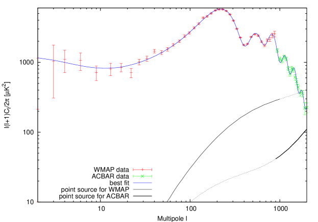
As described, in addition to WMAP 5-year data, we also include ACBAR data at large multipoles. To avoid complicating the analysis when different datasets overlap, which requires a calculation of the covariance matrix between different experiments, as they observe the same sky, in the likelihood calculation, we take the same approach as the WMAP team and use WMAP data out to $\ell<900$ and ACBAR data from $900<\ell<2000$. For ACBAR data, we make a separate estimate of the angular power spectrum by scaling the flux-cut of unresolved point sources to be at the lower flux threshold and in agreement with previous shot-noise estimates reichardt . Again, we include an overall uncertainty in the ACBAR angular power spectrum of radio sources, in this case the sum of clustering and shot-noise terms of the power spectrum, with $P_{\rm ACBAR}$. In Fig. 2, we show the angular power spectrum of CMB anisotropies with best-fit cosmological model for WMAP and ACBAR data, as well as the two input power spectra for point source clustering with both $P_{\rm WMAP}=P_{\rm ACBAR}=1$.

Figure 4: Two-dimensional marginalized distributions showing the $68\%$ and $95\%$ confidence level contours for $n_{s}$ vs. $\Omega_{b}h^{2}$ (left) and $n_{s}$ vs. $\sigma_{8}$ (right) with WMAP 5-years data alone (empty contours), WMAP 5-years data with clustered point sources (red contours), and WMAP 5-years data+ACBAR data with point source clustering (blue contours).

Table 2: Constraints on spectral index $n_{s}$, running of the spectral index ${dn_{s}/d\ln k}$ and tensor to scalar ratio $r$ from WMAP+ACBAR with and without point source signal. These values are evaluated at $k=0.002$ Mpc^-1.

parameter	WMAP+ACBAR	WMAP+ACBAR
		with clustering
ns	$1.036\pm 0.046$	$1.041\pm 0.050$
$dn_{s}/d\ln k$	$-0.038\pm 0.024$	$-0.044\pm 0.025$
ns	$0.981\pm 0.019$	$0.977_{-0.019}^{+0.020}$
r	$<0.36(2\sigma)$	$<0.39(2\sigma)$

Since we only include the clustering term of unresolved point sources for WMAP data, we follow the WMAP team’s approach on the shot-noise term and marginalize the likelihood over the uncertainty related to point source shot-noise term A_ps using the public WMAP likelihood routine. This uncertainty only makes a small difference in best-fit cosmological parameters nolta . The results related to $\Lambda$CDM runs are summarized in Table I. In the case where we do not consider clustering of point sources, we essentially recover the same results as Ref. dunkley , with small differences at the level of 0.1$\sigma$, which we believe is due to differences in the numerical codes and the convergence criteria.

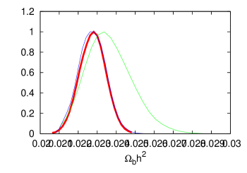
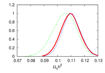
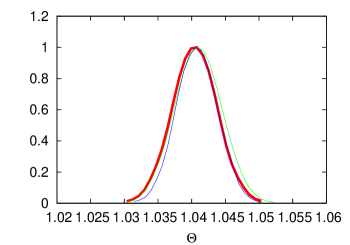
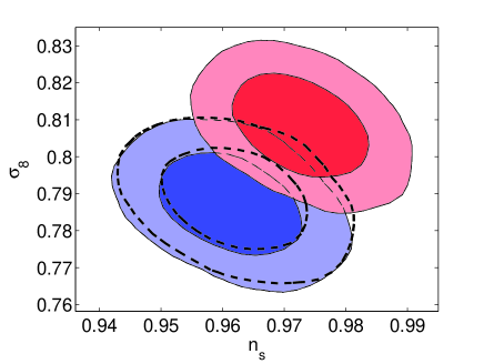
With clustering of point sources included, however, the spectral index estimated with WMAP 5-year data alone changes from $0.965\pm 0.014$ with point source shot-noise only to $0.949\pm 0.018$ with source clustering in addition to the shot-noise from the WMAP likelihood. This is a difference of about $1\sigma$, but this large difference primarily comes from the fact that $P_{\rm WMAP}$ is largely unconstrained by the data with a $2\sigma$ upper limit of 1.38. The change in $n_{s}$ is captured by a similar change in $\sigma_{8}$ with values changing from 0.793 $\pm 0.036$ without clustering to $0.726\pm 0.056$ with clustering. If we put a prior that $P_{\rm WMAP}$ is uniform between 0 and 1, $n_{s}=0.953\pm 0.016$ and the difference from the case with clustering ignored is about $\sim 0.8\sigma$.

Figure 5: Two-dimensional marginalized distributions showing the $68\%$ and $95\%$ confidence level contours for $n_{s}$ vs. $dn_{s}/d\ln k$ (left) and $n_{s}$ vs. $r$ (right) of interest with WMAP 5-year and ACBAR data (empty contours) and and WMAP 5-years data+ACBAR data with clustering for point sources (blue contours).

With the addition of ACBAR data, the clustering amplitudes of unresolved point sources in both WMAP and ACBAR are better constrained. Though we only use WMAP point source clustering model for WMAP data only and a separate model for ACBAR point sources at $\ell>900$, both parameters are better constrained because the combination of WMAP and ACBAR data pin down the overall cosmological model leaving less room for the point source piece to change in amplitude. In combination, with clustering of point sources included for both WMAP and ACBAR, we find $n_{s}=0.959\pm 0.014$, which is different from the WMAP+ACBAR value of $n_{s}=0.963\pm 0.014$ by about 0.3$\sigma$.

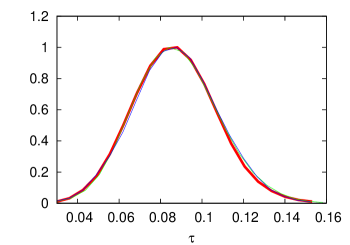
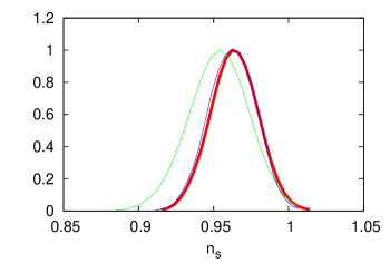
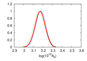
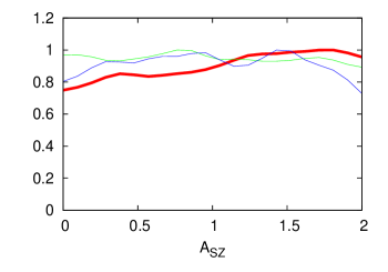
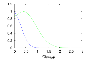
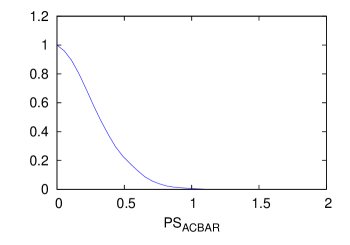
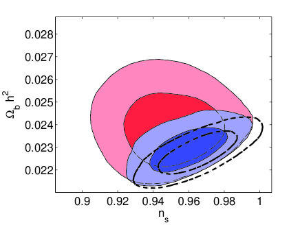
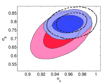
In Fig. 3 we summarize likelihoods of the parameters involved. As shown there, when clustering is included the large differences on cosmological parameter estimates with WMAP data alone appear in $n_{s},\Omega_{b}h^{2}$ and $\Omega_{c}h^{2}$. However, as discussed for $n_{s}$, once we include ACBAR data and with clustering of point sources both for WMAP and ACBAR, the probability distributions are more consistent with the WMAP data alone, but with clustering ignored. While it seems like large multipole data from an experiment such as ACBAR do not improve cosmological parameters estimated from WMAP, in our case, we do see an improvement by constraining the point source clustering amplitude better. The associated contour plots for parameters that are mostly affected by clustering of point sources are summarized in Fig. 4 for combinations of $n_{s}$ vs. $\Omega_{b}h^{2}$ (left) and $n_{s}$ vs. $\sigma_{8}$ (right).

Figure 6: Planck mock data with and without a contribution from point sources: an offset in the temperature power spectrum is visible for small scales. Also showed are the model for point sources used in the paper and a simulated signal for point sources from public point source maps for Planck HFI channels (in this case at 143 GHz) from the Planck team (see text for details).

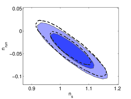
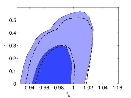
In addition to standard $\Lambda$CDM runs with a power-law power spectrum for density perturbations, we also study the impact of point sources on the running of the spectral index and on the tensor-to-scalar ratio, in addition to the main parameters of the $\Lambda$CDM cosmological model outlined in Table I. In Table II we summarize our results. Our results for the combination of WMAP and ACBAR without clustering are generally consistent with previous results Komatsu5yr , but with minor differences such as a 2$\sigma$ upper limit on $r$ of 0.36 instead of 0.4. The differences between with and without clustering are also minor and this is primarily due to the fact that we take the combination of WMAP and ACBAR. In Fig. 5 we summarize these results in contour plots with $n_{s}$ vs. running (dn${}_{s}/d\ln k$, left) and $n_{s}$ vs. $r$ (right).

Figure 7: Two-dimensional marginalized distributions showing the $68\%$ and $95\%$ confidence level contours for $n_{s}$ vs. $\Omega_{b}h^{2}$ (left) and $n_{s}$ vs. $\sigma_{8}$ (right) in three different cases: Planck mock data alone (empty contours), Planck mock data with clustering for point sources marginalized as a shot-noise (red contours, see text for details), and finally Planck mock data with a clustered point source signal which is marginalized over with a model for clustering. The marginalization over point source clustering in Planck completely removes the bias introduced by the point sources signal and contours overlap.

Table 3: Mean values and marginalized $68\%$ c.l. limits for several cosmological parameters from Planck mock data with and without a point source contribution.

Parameter	Planck mock data	Planck mock data	Planck mock data	Planck mock data
		with clustering	with clustering	with clustering
		Point sources ignored	$C_{l}^{c}\times(0<P_{Planck}<1)$	Shot-noise only ($C_{l}^{sn}=P_{\rm Planck}$)
$\Omega_{b}h^{2}$	$0.02270_{-0.00024}^{+0.00025}$	$0.02753\pm 0.00028$	$0.02271\pm 0.00025$	$0.00271_{-0.00024}^{+0.00025}$
$\Omega_{\rm c}h^{2}$	$0.1082\pm 0.0019$	$0.0924\pm 0.0017$	$0.1080_{-0.0020}^{+0.0019}$	$0.1092_{-0.0019}^{+0.0020}$
$\Omega_{\Lambda}$	$0.750\pm 0.010$	$0.831\pm 0.007$	$0.751_{-0.010}^{+0.011}$	$0.745\pm 0.010$
$n_{s}$	$0.962_{-0.007}^{+0.008}$	$1.159\pm 0.007$	$0.961_{-0.007}^{+0.008}$	$0.973\pm 0.007$
$\tau$	$0.090\pm 0.007$	$0.260_{-0.016}^{+0.015}$	$0.090_{-0.006}^{+0.007}$	$0.094_{-0.008}^{+0.007}$
$\Delta^{2}_{R}$	$(2.41\pm 0.10)\cdot 10^{-9}$	$(1.85\pm 0.10)\cdot 10^{-9}$	$(2.41\pm 0.10)\cdot 10^{-9}$	$(2.40\pm 0.10)\cdot 10^{-9}$
$\sigma_{8}$	$0.789_{-0.009}^{+0.008}$	$0.903_{-0.014}^{+0.015}$	$0.787\pm 0.009$	$0.808\pm 0.009$
$\Omega_{m}$	$0.250\pm 0.010$	$0.169\pm 0.007$	$0.249_{-0.011}^{+0.010}$	$0.255\pm 0.010$
$H_{0}$	$72.4_{-0.9}^{+1.0}$	$84.3_{-1.2}^{+1.1}$	$72.5\pm 1.0$	$72.0\pm 1.0$
$z_{reion}$	$11.3\pm 0.6$	$19.9_{-0.7}^{+0.8}$	$11.3\pm 0.6$	$11.6\pm 0.6$
$t_{0}$	$13.69\pm 0.04$	$13.04_{-0.04}^{+0.05}$	$13.69_{-0.05}^{+0.04}$	$13.70\pm 0.04$
$A_{SZ}$	$1.40\pm 0.07$	$<2.00$	$1.66_{-0.21}^{+0.23}$	$1.84_{-0.14}^{+0.16}$
$P_{\rm Planck}$	$--$	$--$	$<1.00(2\sigma)$	$C_{l}^{\rm sn}<3.6\times 10^{-5}$ $\mu$k2-sr $(2\sigma)$

While we find differences at the level of $1\sigma$ for WMAP data alone with clustering of point sources, our results show that the differences are smaller and insignificant once WMAP data are combined with ACBAR data and using two separate estimates for point source clustering in WMAP and ACBAR data. In future, Planck data will observe CMB anisotropies down to smaller angular scales and extending to higher frequencies where clustering of sources becomes increasingly important Scott ; GonzalezNuevo:2004fj . In this case, it is clear that a simplified approach with a shot-noise for unresolved point sources in Planck data may not be appropriate when extracting cosmological parameters.

III.2 Planck mock data

To understand how clustering of point sources impact cosmological parameter determination, we created several mock datasets with noise properties consistent with Planck 143 GHz channel of HFI and assuming the best-fit WMAP5 parameters Komatsu5yr for cosmology. We model the point source clustering and the shot-noise by making use of existing high-frequency data as we did for ACBAR. While we only consider a single clustering spectrum, at high-frequencies of Planck HFI, two separate populations of point sources are expected: radio, dominating at low-frequencies, and sub-mm or far-IR sources at high-frequencies Amblard . Here, as we only have total number counts at 150 GHz, without any information on hwo to separate the counts to the two populations, we make use of a single clustering spectrum. It will be necessary to return to this topic later once Planck data become available with additional information, from Planck and Herschel, on the far-IR population in HFI channels.

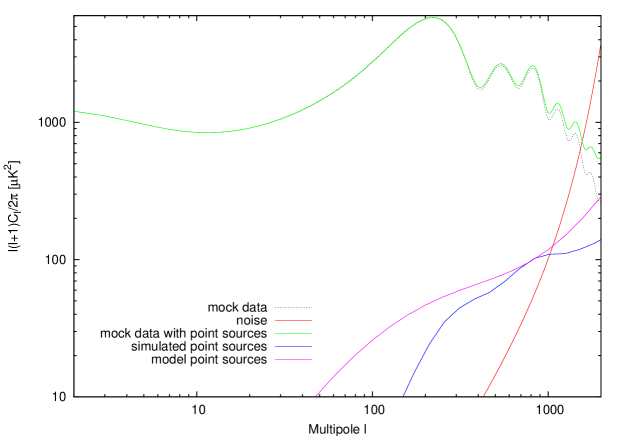
We summarize our results related to Planck data in Fig. 6. In addition to the analytical model of point source clustering used in this paper based on the halo model, we also made use of publicly available Planck source maps from the Planck Working Sub-Group for Compact Source Fields to measure the angular power spectrum of points sources at the Planck HFI 143 GHz channel. These maps are derived from a model based on GalICS model using the Mock Map Facility (MoMaF,blaizotetal05 ). The power spectrum is computed after removing point sources with a flux greater than 72 mJy, 5$\sigma$ detection level of Planck at that frequency according to fernandez08 .

As shown in Fig. 6, while the amplitude of our analytical model matches with the residual clustering spectrum of point sources in the Planck simulation at multipoles of $10^{3}$, our analytical model has residual point sources that are more clustered than the simulated sources. We believe this is due to the finite size of boxes used to simulate the source distribution by the Planck team. While we fix our point sources to the analytical model as shown in Fig. 6, we again capture the uncertainty in the amplitude with a parameter $P_{\rm Planck}$ (in this case clustering and shot-noise combined as in the case of ACBAR data) and marginalize over this parameter when estimating cosmological parameters.

We follow the same procedure as fitting existing WMAP and ACBAR data to extract cosmological parameters with Planck. We use data at $l<2000$, though Planck analysis can be extended to higher multipoles, which are likely to be contaminated by additional secondary anisotropies beyond SZ Cooray5 , and complications of the non-Gaussian covariance Cooray6 . The best-fit cosmological parameters and 68% confidence errors for the standard 6-parameter $\Lambda$CDM case complemented by $A_{\rm SZ}$ and $P_{\rm Planck}$ are tabulated in Table III. Without point sources, we recover the best-fit cosmology that was used to create the mock. Once the mock includes point sources and we ignore the effect of point sources when model fitting the data, we find that the parameters are significantly biased; in some parameters this bias is more than 20$\sigma$. As in the case of current data, we consider the possibility that if it is adequate to model point sources with just a shot-noise power spectrum. We allow $C_{l}^{sn}=P_{\rm Planck}\times 0.0075$ $\mu$k²-sr and fit the data by varying $P_{\rm Planck}$. The values of cosmological parameters with the shot-noise marginalized over is tabulated in Table III, in addition to the 2$\sigma$ upper limit on $C_{l}^{sn}$ from the data. With a shot-noise description only in the model fit, we find biases in cosmological parameters at the level of 1.5$\sigma$, for example, in the case of the spectral index.

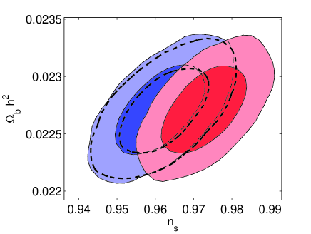
Once we include a model for point source clustering, in addition to the shot-noise, and marginalize over the overall amplitude with our parameter $P_{\rm Planck}$ to capture the overall clustering amplitude, we find that the biases in best-fit parameters from the values used for the mock are removed. We show couple of examples for combinations involving the scalar spectral index $n_{s}$ in Fig. 7 and Fig. 8 for $\Omega_{c}h^{2}$ and $\sigma_{8}$, respectively. As shown, once point source clustering is included in the fit, cosmological parameter biases are negligible. Ignoring point source clustering, however, impacts the measurements significantly, though including only a shot-noise for Planck point sources still results in an appreciable bias. To be completely safe, we suggest that a reasonable model for point source clustering and shot-noise be included in the cosmological parameter analysis with Planck (at each channel used for cosmological measurements) and the uncertainty in the modeling or predicting the total point source contribution be marginalized over.

IV Summary

The faint radio point sources that are unresolved in cosmic microwave background (CMB) anisotropy maps are likely to be a biased tracer of the large-scale structure. While the shot-noise contribution to the angular power spectrum of radio point sources has been considered so far when extracting cosmological parameters with CMB data, we have shown here that one should also allow for the possibility of source clustering. This is especially necessary at high frequencies where the clustering of sources is expected to dominate the shot-noise level of the angular power spectrum at tens of arcminute angular scales. As we find, the differences seen by the WMAP team for V and W-band angular power spectra do allow point source clustering, though one can wrongly conclude clustering is unnecessary if lower frequency data are included.

Here, we have made an estimate of the clustering of unresolved radio sources in both WMAP and ACBAR by making use of existing counts at 95 GHz and by making several assumptions on the sources such as the redshift distribution. To account for the uncertainty in modeling the clustering, we included an extra nuisance parameter for each dataset and have marginalized over this parameter when model fitting for cosmological parameters. For the combination of WMAP 5-year data and ACBAR, we find that the spectral index changes from a mean value of $0.963\pm 0.014$ without point-source clustering to a value of $0.959\pm 0.014$ when the clustering of point sources are included in model fits, a difference of $0.3\sigma$. We also discussed the full parameter set with clustering of radio point sources and changes to additional parameters such as $dn_{s}/d\ln k$ and the tensor-to-scalar ratio $r$. While we find that the differences are marginal with and without source clustering in current data, we have suggested that it is necessary to account for source clustering with future datasets such as Planck, especially to properly model fit anisotropies at arcminute angular scales and using high-frequency data. For Planck, we find that simply including the point sources as a shot-noise only out to $l$ of 2000 for cosmological parameter estimation results in biases at the level of 1.5$\sigma$. While we simply model Planck point sources with a single power spectrum, since at high frequencies both radio and far-IR sources are expected to contribute, it may be necessary to return to a proper model of total unresolved source clustering in Planck in future.

Acknowledgments

This work was supported by NSF CAREER AST-0645427. We thank Mike Nolta for clarifying our questions related to the point source modeling by the WMAP team. AC thanks Dipartimento di Fisica and INFN, Universita’ di Roma-La Sapienza and Aspen Center for Physics for hospitality while this research was completed. AA acknowledges partial support from a McCue fellowship from the UCI Center for Cosmology.