Formulas for the amplitude
of the van der Pol limit cycle

J.L. López S. Abbasbandy R. López-Ruiz Department of Mathematical and Informatics Engineering, Universidad Pública de Navarra, 31006-Pamplona, Spain Department of Mathematics, Science and Research Branch, Islamic Azad University, Tehran, 14778, Iran Department of Mathematics, Imam Khomeini International University, Ghazvin, 34149-16818, Iran Department of Computer Science and BIFI, Universidad de Zaragoza, 50009-Zaragoza, Spain
Abstract

The limit cycle of the van der Pol oscillator, x¨+ϵ(x21)x˙+x=0¨𝑥italic-ϵsuperscript𝑥21˙𝑥𝑥0\ddot{x}+\epsilon(x^{2}-1)\dot{x}+x=0, is studied in the plane (x,x˙)𝑥˙𝑥(x,\dot{x}) by applying the homotopy analysis method. A recursive set of formulas that approximate the amplitude and form of this limit cycle for the whole range of the parameter ϵitalic-ϵ\epsilon is obtained. These formulas generate the amplitude with an error less than 0.1%percent0.10.1\%. To our knowledge, this is the first time where an analytical approximation of the amplitude of the van der Pol limit cycle, with validity from the weakly up to the strongly nonlinear regime, is given.

keywords:
van der Pol oscillator; Homotopy analysis method; Limit cycles PACS numbers: 02.30.Hq, 02.30.Mv, 02.60.Lj
AMS Classification: 34C07, 65L80
journal: This is a draft version dated 

, ,

1 Introduction

The differential equation,

x¨(t)+ϵ(x21)x˙(t)+x(t)=0,t0,formulae-sequence¨𝑥𝑡italic-ϵsuperscript𝑥21˙𝑥𝑡𝑥𝑡0𝑡0\ddot{x}(t)+\epsilon(x^{2}-1)\dot{x}(t)+x(t)=0,\ \ \ t\geq 0, (1.1)

with ϵitalic-ϵ\epsilon a real parameter and the dot denoting the derivative with respect to time t𝑡t, is called the van der Pol oscillator [1]. For ϵ>0italic-ϵ0\epsilon>0, and due to the nonlinear term ϵ(x21)x˙italic-ϵsuperscript𝑥21˙𝑥\epsilon(x^{2}-1)\dot{x}, the system accumulates energy in the region x<1delimited-∣∣𝑥1\mid x\mid<1 and dissipates this energy in the region x>1delimited-∣∣𝑥1\mid x\mid>1. This constraint implies the existence of an stable periodic motion (limit cycle [2]) when ϵ>0italic-ϵ0\epsilon>0. If the nonlinearity is increased, the dynamics in the time domain runs from near-harmonic oscillations when ϵ0italic-ϵ0\epsilon\rightarrow 0 to relaxation oscillations when ϵitalic-ϵ\epsilon\rightarrow\infty, making it a good model for many practical situations [3, 4]. The closed curve representing this oscillation in the plane (x,x˙)𝑥˙𝑥(x,\dot{x}) is quasi circular when ϵ0italic-ϵ0\epsilon\rightarrow 0 and a sharp figure when ϵitalic-ϵ\epsilon\rightarrow\infty. For ϵ<0italic-ϵ0\epsilon<0, the dynamics is dissipative in the region x<1delimited-∣∣𝑥1\mid x\mid<1 and amplificative for x>1delimited-∣∣𝑥1\mid x\mid>1. Under these conditions, the periodic motion is still possible but unstable. In this case, the limit cycle can be derived from that one with ϵ>0italic-ϵ0\epsilon>0 taking into account the symmetry (ϵ,x(t))(ϵ,x(t))italic-ϵ𝑥𝑡italic-ϵ𝑥𝑡(\epsilon,x(t))\rightarrow(-\epsilon,-x(-t)). Therefore, it is enough to study the case ϵ>0italic-ϵ0\epsilon>0 to obtain also the behavior of the system for ϵ<0italic-ϵ0\epsilon<0.

Different standard methods (perturbative, non-perturbative, geometrical) [1, 2, 3, 4, 5, 6, 7] have permitted to study extensively the limit cycle of the van der Pol equation, in the weakly (ϵ0italic-ϵ0\epsilon\rightarrow 0) and in the strongly (ϵitalic-ϵ\epsilon\rightarrow\infty) nonlinear regimes. However, investigations giving analytical information of this object in the intermediate regime (0ϵmuch-less-than0italic-ϵmuch-less-than0\ll\epsilon\ll\infty) are lacking in the literature. In this paper, it is our aim to fill in this gap by applying to the Eq. (1.1) the homotopy analysis method (HAM) introduced by Liao [8, 9] in the nineties. This method has been shown to be powerful to solve different nonlinear problems [10, 11, 12, 13, 14, 15, 16]. In particular, it has been applied in [17] to Liénard equation, x¨+ϵf(x)x˙+x=0¨𝑥italic-ϵ𝑓𝑥˙𝑥𝑥0\ddot{x}+\epsilon f(x)\dot{x}+x=0, which is the generalization of the van der Pol system when f(x)𝑓𝑥f(x) is an arbitrary function. As the interest in that work [17] was the amplitude and the frequency of the periodic motions, the calculations were performed with the time variable being explicit. As here we are only interested in the amplitude and form of the limit cycles, the time dependence of the solutions can be omitted, and we can work directly in the phase space (x,x˙)𝑥˙𝑥(x,\dot{x}). Our results for the van der Pol limit cycle are presented in Section 2. In Section 3 it is explained how these results have been obtained from our specific application of the HAM to the van der Pol equation. Some conclusions are given in the last Section.

2 The amplitude of the van der Pol limit cycle

Nowadays, the amplitude of the van der Pol limit cycle a𝑎a can be easily approximated with a classical Runge-Kutta method. The results of this computational calculation aEsubscript𝑎𝐸a_{E} are shown in Table 1. Let us observe that aE(ϵ)>2subscript𝑎𝐸italic-ϵ2a_{E}(\epsilon)>2 for ϵ>0italic-ϵ0\epsilon>0, with the asymptotic values: aE(ϵ0)=aE(ϵ)=2subscript𝑎𝐸italic-ϵ0subscript𝑎𝐸italic-ϵ2a_{E}(\epsilon\rightarrow 0)=a_{E}(\epsilon\rightarrow\infty)=2. An upper bound rigorously established in [18] for the amplitude a𝑎a is 2.32332.32332.3233. However, as it was signalled there [18], the maximum of aEsubscript𝑎𝐸a_{E} is 2.023422.023422.02342 and it is obtained for ϵ=3.3italic-ϵ3.3\epsilon=3.3. In view of this result, Odani [18] conjectured that the amplitude of the limit cycle of the van der Pol equation is estimated by 2<a(ϵ)<2.02352𝑎italic-ϵ2.02352<a(\epsilon)<2.0235 for every ϵ>0italic-ϵ0\epsilon>0.

ϵitalic-ϵ\epsilon 0.10.10.1 0.50.50.5 1.01.01.0 1.51.51.5 2.02.02.0 2.52.52.5
aEsubscript𝑎𝐸a_{E} 2.00010 2.00249 2.00862 2.01522 2.01989 2.02235
ϵitalic-ϵ\epsilon 3.03.03.0 3.53.53.5 4.04.04.0 5.05.05.0 101010 505050
aEsubscript𝑎𝐸a_{E} 2.02330 2.02337 2.02296 2.02151 2.01428 2.00295

Table 1. The value aEsubscript𝑎𝐸a_{E} represents the amplitude a𝑎a of the van der Pol limit cycle obtained by integrating directly Eq. (1.1) with a Runge-Kutta method for the indicated values of ϵitalic-ϵ\epsilon.

Due to the difficulty of calculating the amplitude a𝑎a by analytical means, one could propose as a good solution the constant amplitude

a¯=2¯𝑎2\bar{a}=2 (2.1)

for the whole range of the parameter ϵitalic-ϵ\epsilon. Knowing that the experimental upper bound for a𝑎a is 2.02342, i.e. 2<a(ϵ)<2.023422𝑎italic-ϵ2.023422<a(\epsilon)<2.02342 for every ϵ>0italic-ϵ0\epsilon>0, the error made with this approximation, (a(ϵ)a¯)/a(ϵ)𝑎italic-ϵ¯𝑎𝑎italic-ϵ(a(\epsilon)-\bar{a})/a(\epsilon), would be about 1%percent11\%.

If more precision is needed, the different analytical expansions in ϵitalic-ϵ\epsilon that have been found for the amplitude in the weakly and in the strongly nonlinear regimes can be considered. Evidently, the error becomes very large in the regions where these approximations are not valid. In [17, 19, 20], a recursive perturbation approximation is used to find the formula for the amplitude when ϵ0italic-ϵ0\epsilon\rightarrow 0. This is, up to order 𝒪(ϵ8)𝒪superscriptitalic-ϵ8\mathcal{O}(\epsilon^{8}),

a(ϵ)ϵ0=2+196ϵ21033552960ϵ4+101968955738368000ϵ6+𝒪(ϵ8).𝑎subscriptitalic-ϵitalic-ϵ02196superscriptitalic-ϵ21033552960superscriptitalic-ϵ4101968955738368000superscriptitalic-ϵ6𝒪superscriptitalic-ϵ8a(\epsilon)_{\epsilon\rightarrow 0}=2+{1\over 96}\ \epsilon^{2}-{1033\over 552960}\ \epsilon^{4}+{1019689\over 55738368000}\ \epsilon^{6}+\mathcal{O}(\epsilon^{8}). (2.2)

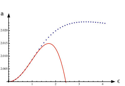
This expansion agrees for small ϵitalic-ϵ\epsilon with the computational calculation aEsubscript𝑎𝐸a_{E} presented in Table 1. For 0<ϵ<20italic-ϵ20<\epsilon<2 the error is less than 1%percent11\%, for ϵ4italic-ϵ4\epsilon\approx 4 the error is bigger than 10%percent1010\%, and for ϵ6italic-ϵ6\epsilon\approx 6 the formula has lost its validity and the error is bigger than 50%percent5050\%. In [21], the asymptotic dependence of the amplitude on ϵitalic-ϵ\epsilon is given for sufficiently large ϵ>0italic-ϵ0\epsilon>0,

a(ϵ)ϵ=2+0.7793ϵ4/3+𝒪¯(ϵ4/3),𝑎subscriptitalic-ϵitalic-ϵ20.7793superscriptitalic-ϵ43¯𝒪superscriptitalic-ϵ43a(\epsilon)_{\epsilon\rightarrow\infty}=2+0.7793\ \epsilon^{-4/3}+\underline{\mathcal{O}}(\epsilon^{-4/3}), (2.3)

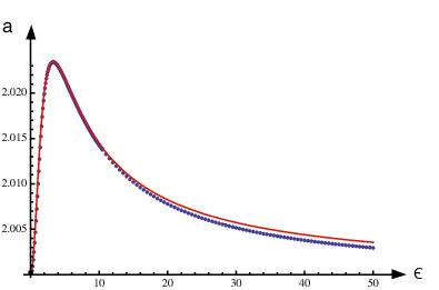
where 𝒪¯¯𝒪\underline{\mathcal{O}} means 𝒪¯(ϵ4/3)<𝒪(ϵ4/3)¯𝒪superscriptitalic-ϵ43𝒪superscriptitalic-ϵ43\underline{\mathcal{O}}(\epsilon^{-4/3})<\mathcal{O}(\epsilon^{-4/3}). Compared with aEsubscript𝑎𝐸a_{E}, this formula generates the amplitude with an error bigger than 15%percent1515\% for ϵ<2italic-ϵ2\epsilon<2. The formula starts to have validity for ϵ10italic-ϵ10\epsilon\approx 10 with an error around 1%percent11\%, that passes to be less than 0.1%percent0.10.1\% when ϵ>50italic-ϵ50\epsilon>50. In Figs. 1.a and 1.b, formulas (2.2) and (2.3) are respectively plotted versus ϵitalic-ϵ\epsilon in their regions of validity.


Refer to caption     Refer to caption

(a)                                                            (b)

Figure 1: Comparison of the ‘experimental’ amplitude aE(ϵ)subscript𝑎𝐸italic-ϵa_{E}(\epsilon) (dotted curve) with (a) amplitude a(ϵ)ϵ0𝑎subscriptitalic-ϵitalic-ϵ0a(\epsilon)_{\epsilon\rightarrow 0} given by formula (2.2) (solid line), and (b) amplitude a(ϵ)ϵ𝑎subscriptitalic-ϵitalic-ϵa(\epsilon)_{\epsilon\rightarrow\infty} given by formula (2.3) (solid line).

We propose here two formulas, aR1(ϵ)subscript𝑎𝑅1italic-ϵa_{R1}(\epsilon) and aR2(ϵ)subscript𝑎𝑅2italic-ϵa_{R2}(\epsilon), that approximate the amplitude of the van der Pol limit cycle for every ϵ>0italic-ϵ0\epsilon>0. The first one with an error less than 0.1%percent0.10.1\%, and the second one with an error less than 0.05%percent0.050.05\%. These formulas have been obtained by applying the HAM to the van der Pol equation. The details of the derivation of these formulas are given in Section 3.

The first formula is

aR1(ϵ)=2+1.737ϵ2(8π+9ϵ)(4+ϵ2),subscript𝑎𝑅1italic-ϵ21.737superscriptitalic-ϵ28𝜋9italic-ϵ4superscriptitalic-ϵ2a_{R1}(\epsilon)=2+{1.737\ \epsilon^{2}\over(8\pi+9\epsilon)(4+\epsilon^{2})}\ , (2.4)

that derives from expression (3.30). The error obtained, |a(ϵ)aR1(ϵ)|/a(ϵ)𝑎italic-ϵsubscript𝑎𝑅1italic-ϵ𝑎italic-ϵ|a(\epsilon)-a_{R1}(\epsilon)|/a(\epsilon), with this formula is less than 0.1%percent0.10.1\% for every ϵ>0italic-ϵ0\epsilon>0. Fig. 2.1 shows aR1subscript𝑎𝑅1a_{R1} in comparison with the ‘experimental’ amplitude aEsubscript𝑎𝐸a_{E}. The maximum of aR1subscript𝑎𝑅1a_{R1} is 2.023172.023172.02317 and it is taken for ϵ=3.3italic-ϵ3.3\epsilon=3.3.

The second formula is

aR2(ϵ)=2+0.74958ϵ2(8π+9ϵ)(4+ϵ2)+ϵ2(75.3562+43.0023ϵ+28.1589ϵ2+8.3479ϵ3)(8π+9ϵ)2(4+ϵ2)2,subscript𝑎𝑅2italic-ϵ20.74958superscriptitalic-ϵ28𝜋9italic-ϵ4superscriptitalic-ϵ2superscriptitalic-ϵ275.356243.0023italic-ϵ28.1589superscriptitalic-ϵ28.3479superscriptitalic-ϵ3superscript8𝜋9italic-ϵ2superscript4superscriptitalic-ϵ22a_{R2}(\epsilon)=2+{0.74958\ \epsilon^{2}\over(8\pi+9\epsilon)(4+\epsilon^{2})}\ +{\epsilon^{2}(75.3562+43.0023\epsilon+28.1589\epsilon^{2}+8.3479\epsilon^{3})\over(8\pi+9\epsilon)^{2}(4+\epsilon^{2})^{2}}\ , (2.5)

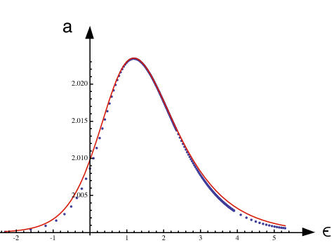
that derives from expression (3.33). The error obtained, |a(ϵ)aR2(ϵ)|/a(ϵ)𝑎italic-ϵsubscript𝑎𝑅2italic-ϵ𝑎italic-ϵ|a(\epsilon)-a_{R2}(\epsilon)|/a(\epsilon), with this formula is less than 0.05%percent0.050.05\% for every ϵ>0italic-ϵ0\epsilon>0. The maximum of aR2subscript𝑎𝑅2a_{R2} is 2.023462.023462.02346 and it is taken for ϵ=3.29482italic-ϵ3.29482\epsilon=3.29482. The plot of aR2subscript𝑎𝑅2a_{R2} in comparison with the amplitude aEsubscript𝑎𝐸a_{E} obtained computationally can be seen in Fig. 2b. Let us observe that it can be guessed from Fig. 2b that aR2(ϵ)>aE(ϵ)subscript𝑎𝑅2italic-ϵsubscript𝑎𝐸italic-ϵa_{R2}(\epsilon)>a_{E}(\epsilon) for every ϵ>0italic-ϵ0\epsilon>0.

The expansion of expression (2.5) for small ϵitalic-ϵ\epsilon gives

aR2(ϵ)ϵ0=2+0.01491ϵ2+𝒪(ϵ3).subscript𝑎𝑅2subscriptitalic-ϵitalic-ϵ020.01491superscriptitalic-ϵ2𝒪superscriptitalic-ϵ3a_{R2}(\epsilon)_{\epsilon\rightarrow 0}=2+0.01491\ \epsilon^{2}+{\mathcal{O}}(\epsilon^{3}). (2.6)

For large ϵitalic-ϵ\epsilon, we obtain

aR2(ϵ)ϵ=2+0.18648ϵ1+𝒪(ϵ2).subscript𝑎𝑅2subscriptitalic-ϵitalic-ϵ20.18648superscriptitalic-ϵ1𝒪superscriptitalic-ϵ2a_{R2}(\epsilon)_{\epsilon\rightarrow\infty}=2+{0.18648\ \epsilon^{-1}}+{\mathcal{O}}(\epsilon^{-2}). (2.7)

Let us note the different scaling of this last expression (with behavior ϵ1superscriptitalic-ϵ1\epsilon^{-1}) respect to expansion (2.3) (with behavior ϵ1.33superscriptitalic-ϵ1.33\epsilon^{-1.33}). Taking into account that these approximations start to be valid when ϵ>100italic-ϵ100\epsilon>100, it can be easily seen that this difference is negligible, in fact less than 0.01%percent0.010.01\%. Nevertheless, we have tried to modify formula (2.5) to obtain the correct scaling ϵ1.33superscriptitalic-ϵ1.33\epsilon^{-1.33} of expression (2.3), but the increase of the error in other regions of the parameter ϵitalic-ϵ\epsilon does not recommend this possibility.

In summary, let us remark the exceptional fit of the ‘experimental’ points aEsubscript𝑎𝐸a_{E} by the amplitudes aR1subscript𝑎𝑅1a_{R1} and aR2subscript𝑎𝑅2a_{R2} generated with formulas (2.4) and (2.5), respectively (see Figs. 2a and 2b). Moreover, by inspection of Fig. 2b, let us finish this section by posing the following

Conjecture: the amplitude aR2(ϵ)subscript𝑎𝑅2italic-ϵa_{R2}(\epsilon) obtained with formula (2.5) is an upper bound for the amplitude a(ϵ)𝑎italic-ϵa(\epsilon) of the van der Pol limit cycle, that is

aR2(ϵ)>a(ϵ)foreveryϵ>0.formulae-sequencesubscript𝑎𝑅2italic-ϵ𝑎italic-ϵ𝑓𝑜𝑟𝑒𝑣𝑒𝑟𝑦italic-ϵ0a_{R2}(\epsilon)>a(\epsilon)\ \ for\ every\ \ \epsilon>0. (2.8)

Refer to caption     Refer to caption

(a)                                                            (b)

Figure 2: (a) Amplitude aR1(ϵ)subscript𝑎𝑅1italic-ϵa_{R1}(\epsilon) given by formula (2.4) (solid curve), and experimental amplitude aE(ϵ)subscript𝑎𝐸italic-ϵa_{E}(\epsilon). (b) Amplitude aR2(ϵ)subscript𝑎𝑅2italic-ϵa_{R2}(\epsilon) given by formula (2.5) (solid curve), and experimental amplitude aE(ϵ)subscript𝑎𝐸italic-ϵa_{E}(\epsilon) (dotted curve), and ϵitalic-ϵ\epsilon given in logarithmic scale.

3 The HAM and the van der Pol equation

The generalization of the van der Pol equation, u¨+ϵ(u21)u˙+u=0¨𝑢italic-ϵsuperscript𝑢21˙𝑢𝑢0\ddot{u}+\epsilon(u^{2}-1)\dot{u}+u=0, is called the Liénard equation. In coordinates (u,v)𝑢𝑣(u,v), it reads

u¨(t)+ϵf(u)u˙(t)+u(t)=0,t0,formulae-sequence¨𝑢𝑡italic-ϵ𝑓𝑢˙𝑢𝑡𝑢𝑡0𝑡0\ddot{u}(t)+\epsilon f(u)\dot{u}(t)+u(t)=0,\ \ \ t\geq 0, (3.1)

where we consider that f(u)𝑓𝑢f(u) is an even function. The HAM has been applied to this equation in [17] working explicitly in the time domain. We proceed now to apply the HAM to this system by following a different strategy, namely, by omitting the time variable of Eq. (3.1).

3.1 HAM applied to Liénard equation

If we define the variable v=u˙𝑣˙𝑢v=\dot{u}, and suppose that v𝑣v is a function of u𝑢u, the acceleration u¨¨𝑢\ddot{u} can be rewritten as vvsuperscript𝑣𝑣v^{\prime}v, where the prime denotes the derivative respect to u𝑢u. The result is a new equation with the time variable eliminated:

vv+ϵf(u)v+u=0.𝑣superscript𝑣italic-ϵ𝑓𝑢𝑣𝑢0vv^{\prime}+\epsilon f(u)v+u=0. (3.2)

When f(u)𝑓𝑢f(u) is even [22, 23], the limit cycles of this equation are closed trajectories of amplitude a𝑎a in the (u,v)𝑢𝑣(u,v) plane, with aua𝑎𝑢𝑎-a\leq u\leq a and v(a)=v(a)=0𝑣𝑎𝑣𝑎0v(a)=v(-a)=0.

After the re-scaling (u,v)=(ax,ay)𝑢𝑣𝑎𝑥𝑎𝑦(u,v)=(ax,ay) to the new variables (x,y)𝑥𝑦(x,y), the limit cycles are transformed in solutions of the equation

yy+ϵyf(ax)+x=0,1x1,y(1)=y(1)=0,formulae-sequenceformulae-sequence𝑦superscript𝑦italic-ϵ𝑦𝑓𝑎𝑥𝑥01𝑥1𝑦1𝑦10yy^{\prime}+\epsilon yf(ax)+x=0,\hskip 28.45274pt-1\leq x\leq 1,\hskip 28.45274pty(-1)=y(1)=0, (3.3)

where the prime is now denoting the derivative respect to x𝑥x.

From [22, 23], we know that an approximate solution of the positive branch solution of (3.3), for any value of ϵ>0italic-ϵ0\epsilon>0, is

y~(x)=1x2+ϵa~{0if1x<x0/a~F(a~)F(a~x)ifx0/a~x1,~𝑦𝑥1superscript𝑥2italic-ϵ~𝑎cases0𝑖𝑓1𝑥subscript𝑥0~𝑎𝐹~𝑎𝐹~𝑎𝑥𝑖𝑓subscript𝑥0~𝑎𝑥1\tilde{y}(x)=\sqrt{1-x^{2}}+{\epsilon\over\tilde{a}}\left\{\begin{array}[]{ll}0\hskip 56.9055pt&{if}\hskip 5.69054pt-1\leq x<x_{0}/\tilde{a}\\ F(\tilde{a})-F(\tilde{a}x)\hskip 14.22636pt&{if}\hskip 5.69054ptx_{0}/\tilde{a}\leq x\leq 1,\end{array}\right. (3.4)

where F(x)=f(x)superscript𝐹𝑥𝑓𝑥F^{\prime}(x)=f(x), x0subscript𝑥0x_{0} is a negative root of f(x)𝑓𝑥f(x): f(x0)=0𝑓subscript𝑥00f(x_{0})=0 with x0<0subscript𝑥00x_{0}<0, and a~~𝑎\tilde{a} is a positive root of F(x0)F(x)𝐹subscript𝑥0𝐹𝑥F(x_{0})-F(x): F(x0)=F(a~)𝐹subscript𝑥0𝐹~𝑎F(x_{0})=F(\tilde{a}) with a~>0~𝑎0\tilde{a}>0. The number of possible stable limit cycles in the strongly non-linear regime (for large ϵitalic-ϵ\epsilon) is obtained from the number of positive roots of F(x0)F(x)𝐹subscript𝑥0𝐹𝑥F(x_{0})-F(x) when x0subscript𝑥0x_{0} runs over the set of all the negative roots of f(x0)=0𝑓subscript𝑥00f(x_{0})=0. We take the positive roots a~~𝑎\tilde{a} selected by the algorithm explained in [22, 23] as the corresponding approximate amplitudes. Let us observe that the initial approximate limit cycle y~(x)~𝑦𝑥\tilde{y}(x) recovers the exact circular form when ϵ0italic-ϵ0\epsilon\rightarrow 0, and also, when ϵitalic-ϵ\epsilon\rightarrow\infty, it becomes exactly the two-piecewise limit cycle proposed in [22]. Moreover, it must be noticed that y~(x)~𝑦𝑥\tilde{y}(x) has sense only when ϵ>0italic-ϵ0\epsilon>0, and then the results obtained from this initial guess only will have validity for ϵ>0italic-ϵ0\epsilon>0.

After eliminating the time variable, the non-linear differential equation yy+ϵyf(ax)+x=0𝑦superscript𝑦italic-ϵ𝑦𝑓𝑎𝑥𝑥0yy^{\prime}+\epsilon yf(ax)+x=0 is of order one. Then, to construct the homotopy [8, 9], we build a linear differential equation of order one for the whole range [0,1]01[0,1] of what is called the homotopy parameter p𝑝p.

We define an auxiliary linear operator {\mathcal{L}} by

[ϕ(x;p)]=xϕ(x;p),delimited-[]italic-ϕ𝑥𝑝𝑥italic-ϕ𝑥𝑝{\mathcal{L}}[\phi(x;p)]=\frac{\partial}{\partial x}\phi(x;p), (3.5)

with the property

[C1]=0,delimited-[]subscript𝐶10{\mathcal{L}}[C_{1}]=0, (3.6)

where C1subscript𝐶1C_{1} is a constant, and p𝑝p is a (homotopy) parameter explained below.

From (3.3) we define a nonlinear operator

𝒩[ϕ(x;p),A(p)]=ϕ(x;p)ϕ(x;p)x+ϵϕ(x;p)f(A(p)x)+x,𝒩italic-ϕ𝑥𝑝𝐴𝑝italic-ϕ𝑥𝑝italic-ϕ𝑥𝑝𝑥italic-ϵitalic-ϕ𝑥𝑝𝑓𝐴𝑝𝑥𝑥{\mathcal{N}}[\phi(x;p),A(p)]=\phi(x;p)\frac{\partial\phi(x;p)}{\partial x}+\epsilon\phi(x;p)f(A(p)x)+x, (3.7)

and then construct the homotopy

[ϕ(x;p),A(p)]=(1p)[ϕ(x;p)y~(x)]+hp𝒩[ϕ(x;p),A(p)],italic-ϕ𝑥𝑝𝐴𝑝1𝑝delimited-[]italic-ϕ𝑥𝑝~𝑦𝑥𝑝𝒩italic-ϕ𝑥𝑝𝐴𝑝{\mathcal{H}}[\phi(x;p),A(p)]=(1-p){\mathcal{L}}[\phi(x;p)-\tilde{y}(x)]+hp{\mathcal{N}}[\phi(x;p),A(p)], (3.8)

where hh is a nonzero auxiliary parameter. Setting [ϕ(x;p),A(p)]=0italic-ϕ𝑥𝑝𝐴𝑝0{\mathcal{H}}[\phi(x;p),A(p)]=0, we have the zero-order deformation equation

(1p)[ϕ(x;p)y~(x)]+hp𝒩[ϕ(x;p),A(p)]=0,1𝑝delimited-[]italic-ϕ𝑥𝑝~𝑦𝑥𝑝𝒩italic-ϕ𝑥𝑝𝐴𝑝0(1-p){\mathcal{L}}[\phi(x;p)-\tilde{y}(x)]+hp{\mathcal{N}}[\phi(x;p),A(p)]=0, (3.9)

subject to the boundary conditions

ϕ(1;p)=0,ϕ(1;p)=0,formulae-sequenceitalic-ϕ1𝑝0italic-ϕ1𝑝0\phi(-1;p)=0,\qquad\phi(1;p)=0, (3.10)

where p[0,1]𝑝01p\in[0,1] is an embedding parameter. When the parameter p𝑝p increases from 0 to 1, the solution ϕ(x;p)italic-ϕ𝑥𝑝\phi(x;p) varies from y0(x)=y~(x)subscript𝑦0𝑥~𝑦𝑥y_{0}(x)=\tilde{y}(x) to y(x)𝑦𝑥y(x), A(p)𝐴𝑝A(p) varies from a0subscript𝑎0a_{0} to a𝑎a. Assume that ϕ(x;p)italic-ϕ𝑥𝑝\phi(x;p) and A(p)𝐴𝑝A(p) are analytic in p[0,1]𝑝01p\in[0,1] and can be expanded in the Maclaurin series of p𝑝p as follows:

ϕ(x;p)=n=0+yn(x)pn,A(p)=n=0+anpn,formulae-sequenceitalic-ϕ𝑥𝑝superscriptsubscript𝑛0subscript𝑦𝑛𝑥superscript𝑝𝑛𝐴𝑝superscriptsubscript𝑛0subscript𝑎𝑛superscript𝑝𝑛\phi(x;p)=\sum_{n=0}^{+\infty}y_{n}(x)p^{n},\ \ A(p)=\sum_{n=0}^{+\infty}a_{n}p^{n}, (3.11)

where

yn(x)=1n!nϕ(x;p)pn|p=0,an=1n!nA(p)pn|p=0.formulae-sequencesubscript𝑦𝑛𝑥evaluated-at1𝑛superscript𝑛italic-ϕ𝑥𝑝superscript𝑝𝑛𝑝0subscript𝑎𝑛evaluated-at1𝑛superscript𝑛𝐴𝑝superscript𝑝𝑛𝑝0y_{n}(x)=\frac{1}{n!}\frac{\partial^{n}\phi(x;p)}{\partial p^{n}}\Big{|}_{p=0},\qquad a_{n}=\frac{1}{n!}\frac{\partial^{n}A(p)}{\partial p^{n}}\Big{|}_{p=0}.

Notice that series (3.11) contain the auxiliary parameter hh, which has influence on their convergence regions. Assume that hh is properly chosen such that all of these Maclaurin series are convergent at p=1𝑝1p=1. Hence at p=1𝑝1p=1 we have

y(x)=y0(x)+n=1+yn(x),a=a0+n=1+an.formulae-sequence𝑦𝑥subscript𝑦0𝑥superscriptsubscript𝑛1subscript𝑦𝑛𝑥𝑎subscript𝑎0superscriptsubscript𝑛1subscript𝑎𝑛y(x)=y_{0}(x)+\sum_{n=1}^{+\infty}y_{n}(x),\qquad a=a_{0}+\sum_{n=1}^{+\infty}a_{n}.

At the N𝑁Nth-order approximation, we have the analytic solution of Eq. (3.3), namely

y(x)YN(x):=n=0Nyn(x),aAN:=n=0Nan.formulae-sequence𝑦𝑥subscript𝑌𝑁𝑥assignsuperscriptsubscript𝑛0𝑁subscript𝑦𝑛𝑥𝑎subscript𝐴𝑁assignsuperscriptsubscript𝑛0𝑁subscript𝑎𝑛y(x)\approx Y_{N}(x):=\sum_{n=0}^{N}y_{n}(x),\ \ a\approx A_{N}:=\sum_{n=0}^{N}a_{n}. (3.12)

The parameter hh is free and can be chosen arbitrarily, in particular, it can be a function of ϵitalic-ϵ\epsilon. Nevertheless, the function y~(x)~𝑦𝑥\tilde{y}(x) is the exact limit cycle solution of the Liénard equation (3.3) in the limits ϵ0italic-ϵ0\epsilon\to 0 and ϵitalic-ϵ\epsilon\to\infty. This means that the general solution y(x,h)𝑦𝑥y(x,h) of Eq. (3.9) should tend to y~(x)~𝑦𝑥\tilde{y}(x) for any p𝑝p in those limits of ϵitalic-ϵ\epsilon, loosing its dependence on hh. Then, a reasonable property for hh would be to vanish in those limits of ϵitalic-ϵ\epsilon. Hence, the solution of (3.9) would be the exact solution y~(x)~𝑦𝑥\tilde{y}(x) for any value of the parameter p𝑝p in the limits ϵ0italic-ϵ0\epsilon\to 0 and ϵitalic-ϵ\epsilon\to\infty. A simple function h(ϵ)italic-ϵh(\epsilon) satisfying these properties is

h(ϵ)=bϵc+ϵ2,withb,cR.formulae-sequenceitalic-ϵ𝑏italic-ϵ𝑐superscriptitalic-ϵ2𝑤𝑖𝑡𝑏𝑐𝑅h(\epsilon)={b\epsilon\over c+\epsilon^{2}},\hskip 14.22636ptwith\hskip 14.22636ptb,c\in R. (3.13)

Differentiating Eqs. (3.9) and (3.10) n𝑛n times with respect to p𝑝p, then setting p=0𝑝0p=0, and finally dividing by n!𝑛n!\,, we obtain the n𝑛nth-order deformation equation

[yn(x)χnyn1(x)]+hRn(x)=0,(n=1,2,3,),delimited-[]subscript𝑦𝑛𝑥subscript𝜒𝑛subscript𝑦𝑛1𝑥subscript𝑅𝑛𝑥0𝑛123{\mathcal{L}}[y_{n}(x)-\chi_{n}y_{n-1}(x)]+hR_{n}(x)=0,\qquad(n=1,2,3,\ldots), (3.14)

subject to the boundary conditions

yn(1)=0,yn(1)=0,formulae-sequencesubscript𝑦𝑛10subscript𝑦𝑛10y_{n}(-1)=0,\quad y_{n}(1)=0, (3.15)

where Rn(x)subscript𝑅𝑛𝑥R_{n}(x) is defined by

Rn(x)=1(n1)!n1𝒩[ϕ(x;p),A(p)]pn1|p=0,subscript𝑅𝑛𝑥evaluated-at1𝑛1superscript𝑛1𝒩italic-ϕ𝑥𝑝𝐴𝑝superscript𝑝𝑛1𝑝0R_{n}(x)={1\over(n-1)!}{\partial^{n-1}{\mathcal{N}}[\phi(x;p),A(p)]\over\partial p^{n-1}}\Big{|}_{p=0}, (3.16)

and

χn={0,n1,1,n>1.subscript𝜒𝑛cases0𝑛11𝑛1\chi_{n}=\left\{\begin{array}[]{ll}0,&n\leq 1,\\ 1,&n>1.\end{array}\right.

At each iteration, we have two unknowns, C1subscript𝐶1C_{1}, in Eq. (3.6), and ansubscript𝑎𝑛a_{n}. These unknowns are obtained by considering the boundary conditions (3.15) as follows.

At zero order, we obtain

y0(x)=y~(x).subscript𝑦0𝑥~𝑦𝑥y_{0}(x)=\tilde{y}(x). (3.17)

At 1th-order, we obtain

y1(x)=h2[1x2y02(x)]hϵ1xy0(t)f(a0t)𝑑t,subscript𝑦1𝑥2delimited-[]1superscript𝑥2superscriptsubscript𝑦02𝑥italic-ϵsuperscriptsubscript1𝑥subscript𝑦0𝑡𝑓subscript𝑎0𝑡differential-d𝑡y_{1}(x)={h\over 2}\left[1-x^{2}-y_{0}^{2}(x)\right]-h\epsilon\int_{-1}^{x}y_{0}(t)f(a_{0}t)dt, (3.18)

where we have imposed the condition y1(1)=0subscript𝑦110y_{1}(-1)=0 choosing the integration constant, C1subscript𝐶1C_{1}, appropriately. At this moment a0subscript𝑎0a_{0} is free, but we can fix the value of a0subscript𝑎0a_{0} by imposing y1(1)=0subscript𝑦110y_{1}(1)=0:

11y0(t)f(a0t)𝑑t=0.superscriptsubscript11subscript𝑦0𝑡𝑓subscript𝑎0𝑡differential-d𝑡0\int_{-1}^{1}y_{0}(t)f(a_{0}t)dt=0. (3.19)

This is a non linear equation for a0subscript𝑎0a_{0}. When f(x)𝑓𝑥f(x) is an even polynomial of degree 2n2𝑛2n, it is a polynomial equation of degree n𝑛n in the variable a02superscriptsubscript𝑎02a_{0}^{2}. Therefore, at this order, the number of limit cycles is the number of positive roots of this equation, at most n𝑛n (see [23] for a longer discussion of this point).

Then, for every one of the a0subscript𝑎0a_{0} solutions of the above equation, i.e. for every one of the limit cycles of the system, we proceed order by order in p𝑝p to obtain higher order corrections to the amplitude a𝑎a and to the shape of the limit cycle y(x)𝑦𝑥y(x). At any n𝑛nth-order, with n2𝑛2n\geq 2, we obtain the n𝑛nth-order correction ynsubscript𝑦𝑛y_{n} to the shape of the limit cycle:

yn(x)=yn1(x)h2k=0n1yk(x)ynk1(x)ϵh1xyn1(t)f(a0t)𝑑tϵhk=1n11xynk1(t)m=1kBk,m(a1,a2,,ak)m!tmf(m)(a0t)dt,subscript𝑦𝑛𝑥absentsubscript𝑦𝑛1𝑥2superscriptsubscript𝑘0𝑛1subscript𝑦𝑘𝑥subscript𝑦𝑛𝑘1𝑥italic-ϵsuperscriptsubscript1𝑥subscript𝑦𝑛1𝑡𝑓subscript𝑎0𝑡differential-d𝑡missing-subexpressionitalic-ϵsuperscriptsubscript𝑘1𝑛1superscriptsubscript1𝑥subscript𝑦𝑛𝑘1𝑡superscriptsubscript𝑚1𝑘subscript𝐵𝑘𝑚subscript𝑎1subscript𝑎2subscript𝑎𝑘𝑚superscript𝑡𝑚superscript𝑓𝑚subscript𝑎0𝑡𝑑𝑡\begin{array}[]{ll}y_{n}(x)=&\displaystyle{y_{n-1}(x)-{h\over 2}\sum_{k=0}^{n-1}y_{k}(x)y_{n-k-1}(x)-\epsilon h\int_{-1}^{x}y_{n-1}(t)f(a_{0}t)dt}\\ &\displaystyle{-\epsilon h\sum_{k=1}^{n-1}\int_{-1}^{x}y_{n-k-1}(t)\sum_{m=1}^{k}{B_{k,m}(a_{1},a_{2},...,a_{k})\over m!}t^{m}f^{(m)}(a_{0}t)dt,}\end{array} (3.20)

where Bn,m(a1,,an)subscript𝐵𝑛𝑚subscript𝑎1subscript𝑎𝑛B_{n,m}(a_{1},...,a_{n}) are the partial ordinary Bell polynomials [[24], p. 190]. We have B0,0=1subscript𝐵001B_{0,0}=1 and, for n=1,2,3,𝑛123n=1,2,3,..., Bn+1,0=0subscript𝐵𝑛100B_{n+1,0}=0 and they satisfy the recurrence

Bn,m(a1,,an)=k=m1n1ankBk,m1(a1,,an).subscript𝐵𝑛𝑚subscript𝑎1subscript𝑎𝑛superscriptsubscript𝑘𝑚1𝑛1subscript𝑎𝑛𝑘subscript𝐵𝑘𝑚1subscript𝑎1subscript𝑎𝑛B_{n,m}(a_{1},...,a_{n})=\sum_{k=m-1}^{n-1}a_{n-k}B_{k,m-1}(a_{1},...,a_{n}). (3.21)

We recall that Bn,m(a1,,an)subscript𝐵𝑛𝑚subscript𝑎1subscript𝑎𝑛B_{n,m}(a_{1},...,a_{n}) is linear in ansubscript𝑎𝑛a_{n}.

At n𝑛nth-order, we can obtain also the n𝑛nth-order correction an1subscript𝑎𝑛1a_{n-1} to the amplitude of the limit cycle by imposing the condition yn(1)=0subscript𝑦𝑛10y_{n}(1)=0. The result is a linear equation for an1subscript𝑎𝑛1a_{n-1} with solution:

an1=[11yn1(x)f(a0x)𝑑x+k=1n1m=1kynk1(x)Bk,m(a1,,ak)m!xmf(m)(a0x)dx]/[11xy0(x)f(a0x)𝑑x],subscript𝑎𝑛1absentdelimited-[]superscriptsubscript11subscript𝑦𝑛1𝑥𝑓subscript𝑎0𝑥differential-d𝑥superscriptsubscript𝑘1𝑛1superscriptsuperscriptsubscript𝑚1𝑘subscript𝑦𝑛𝑘1𝑥subscript𝐵𝑘𝑚subscript𝑎1subscript𝑎𝑘𝑚superscript𝑥𝑚superscript𝑓𝑚subscript𝑎0𝑥𝑑𝑥missing-subexpression/absentdelimited-[]superscriptsubscript11𝑥subscript𝑦0𝑥superscript𝑓subscript𝑎0𝑥differential-d𝑥\begin{array}[]{ll}a_{n-1}=&-\left[\displaystyle{\int_{-1}^{1}y_{n-1}(x)f(a_{0}x)dx+\sum_{k=1}^{n-1}{\sum_{m=1}^{k}}^{*}y_{n-k-1}(x){B_{k,m}(a_{1},...,a_{k})\over m!}x^{m}f^{(m)}(a_{0}x)dx}\right]\\ &\hskip 14.22636pt\left/\left[\displaystyle{\int_{-1}^{1}xy_{0}(x)f^{\prime}(a_{0}x)dx}\right],\right.\end{array} (3.22)

where the star in the sum symbol means that the term (k,m)=(n1,1)𝑘𝑚𝑛11(k,m)=(n-1,1) is excluded.

For example, at 2th-order we obtain

y2(x)=y1(x)hy0(x)y1(x)hϵ1x[y1(t)f(a0t)+ty0(t)f(a0t)a1]𝑑tsubscript𝑦2𝑥subscript𝑦1𝑥subscript𝑦0𝑥subscript𝑦1𝑥italic-ϵsuperscriptsubscript1𝑥delimited-[]subscript𝑦1𝑡𝑓subscript𝑎0𝑡𝑡subscript𝑦0𝑡superscript𝑓subscript𝑎0𝑡subscript𝑎1differential-d𝑡y_{2}(x)=y_{1}(x)-hy_{0}(x)y_{1}(x)-h\epsilon\int_{-1}^{x}[y_{1}(t)f(a_{0}t)+ty_{0}(t)f^{\prime}(a_{0}t)a_{1}]dt (3.23)

and

a1=[11y1(x)f(a0x)𝑑x]/[11xy0(x)f(a0x)𝑑x].subscript𝑎1/delimited-[]superscriptsubscript11subscript𝑦1𝑥𝑓subscript𝑎0𝑥differential-d𝑥delimited-[]superscriptsubscript11𝑥subscript𝑦0𝑥superscript𝑓subscript𝑎0𝑥differential-d𝑥a_{1}=-\left[\int_{-1}^{1}y_{1}(x)f(a_{0}x)dx\right]\left/\left[\int_{-1}^{1}xy_{0}(x)f^{\prime}(a_{0}x)dx\right].\right. (3.24)

Therefore, a first approximation to the shape of the limit cycle is y0(x)+y1(x)subscript𝑦0𝑥subscript𝑦1𝑥y_{0}(x)+y_{1}(x), and a first order approximation to the amplitude of the limit cycle is a=a0+a1𝑎subscript𝑎0subscript𝑎1a=a_{0}+a_{1}.

At 3th-order, we have

y3(x)=y2(x)hy0(x)y2(x)h2y12(x)hϵ1x[y2(t)f(a0t)+a1ty1(t)f(a0t)+12a12t2y0(t)f′′(a0t)+ty0(t)f(a0t)a2]𝑑tsubscript𝑦3𝑥absentsubscript𝑦2𝑥subscript𝑦0𝑥subscript𝑦2𝑥2superscriptsubscript𝑦12𝑥missing-subexpressionitalic-ϵsuperscriptsubscript1𝑥delimited-[]subscript𝑦2𝑡𝑓subscript𝑎0𝑡subscript𝑎1𝑡subscript𝑦1𝑡superscript𝑓subscript𝑎0𝑡12superscriptsubscript𝑎12superscript𝑡2subscript𝑦0𝑡superscript𝑓′′subscript𝑎0𝑡𝑡subscript𝑦0𝑡superscript𝑓subscript𝑎0𝑡subscript𝑎2differential-d𝑡\begin{array}[]{ll}y_{3}(x)=&\displaystyle{y_{2}(x)-hy_{0}(x)y_{2}(x)-{h\over 2}y_{1}^{2}(x)}\\ &\hskip-28.45274pt\displaystyle{-h\epsilon\int_{-1}^{x}\left[y_{2}(t)f(a_{0}t)+a_{1}ty_{1}(t)f^{\prime}(a_{0}t)+{1\over 2}a_{1}^{2}t^{2}y_{0}(t)f^{\prime\prime}(a_{0}t)+ty_{0}(t)f^{\prime}(a_{0}t)a_{2}\right]dt}\end{array} (3.25)

and

a2=[11[y2(x)f(a0x)+a1xy1(x)f(a0x)+12a12x2y0(x)f′′(a0x)]𝑑x]/[11xy0(x)f(a0x)𝑑x].subscript𝑎2absentdelimited-[]superscriptsubscript11delimited-[]subscript𝑦2𝑥𝑓subscript𝑎0𝑥subscript𝑎1𝑥subscript𝑦1𝑥superscript𝑓subscript𝑎0𝑥12superscriptsubscript𝑎12superscript𝑥2subscript𝑦0𝑥superscript𝑓′′subscript𝑎0𝑥differential-d𝑥missing-subexpression/absentdelimited-[]superscriptsubscript11𝑥subscript𝑦0𝑥superscript𝑓subscript𝑎0𝑥differential-d𝑥\begin{array}[]{ll}a_{2}=&\displaystyle{-\left[\int_{-1}^{1}\left[y_{2}(x)f(a_{0}x)+a_{1}xy_{1}(x)f^{\prime}(a_{0}x)+{1\over 2}a_{1}^{2}x^{2}y_{0}(x)f^{\prime\prime}(a_{0}x)\right]dx\right]}\\ &\hskip 14.22636pt\left/\displaystyle{\left[\int_{-1}^{1}xy_{0}(x)f^{\prime}(a_{0}x)dx\right].}\right.\end{array} (3.26)

Therefore, a second order approximation to the shape of the limit cycle is y0(x)+y1(x)+y2(x)subscript𝑦0𝑥subscript𝑦1𝑥subscript𝑦2𝑥y_{0}(x)+y_{1}(x)+y_{2}(x) and a second order approximation to the amplitude of the limit cycle is a=a0+a1+a2𝑎subscript𝑎0subscript𝑎1subscript𝑎2a=a_{0}+a_{1}+a_{2}.

Moreover, at every order in p𝑝p the appropriate function h(ϵ)italic-ϵh(\epsilon) is indicated by the experiment.

3.2 Results for the van der Pol equation

For the van der Pol system, we have f(x)=x21𝑓𝑥superscript𝑥21f(x)=x^{2}-1, F(x)=x3/3x𝐹𝑥superscript𝑥33𝑥F(x)=x^{3}/3-x, x0=1subscript𝑥01x_{0}=-1, a~=2~𝑎2\tilde{a}=2 and

y~(x)=1x2+ϵ2{0if1x<1/2,F(2)F(2x)if1/2x1.~𝑦𝑥1superscript𝑥2italic-ϵ2cases0𝑖𝑓1𝑥12𝐹2𝐹2𝑥𝑖𝑓12𝑥1\tilde{y}(x)=\sqrt{1-x^{2}}+{\epsilon\over 2}\left\{\begin{array}[]{ll}0\hskip 56.9055pt&{if}\hskip 5.69054pt-1\leq x<-1/2,\\ F(2)-F(2x)\hskip 14.22636pt&{if}\hskip 5.69054pt-1/2\leq x\leq 1.\end{array}\right. (3.27)

The expressions for yn(x)subscript𝑦𝑛𝑥y_{n}(x) given by the recursive formula (3.20) can be calculated with Mathematica. Although they are elementary functions, their length is excessive to be reproduced here. From (3.19) we get

11y0(t)f(a0t)𝑑t=9ϵ+8π64(a024)=0a0=2.superscriptsubscript11subscript𝑦0𝑡𝑓subscript𝑎0𝑡differential-d𝑡9italic-ϵ8𝜋64superscriptsubscript𝑎0240subscript𝑎02\int_{-1}^{1}y_{0}(t)f(a_{0}t)dt={9\epsilon+8\pi\over 64}(a_{0}^{2}-4)=0\Longrightarrow a_{0}=2. (3.28)

From (3.24) we obtain

a1(h)=273ϵh35(8π+9ϵ).subscript𝑎1273italic-ϵ358𝜋9italic-ϵa_{1}(h)=-{27\sqrt{3}\epsilon h\over 35(8\pi+9\epsilon)}. (3.29)

Therefore, a first approximation to the amplitude of the limit cycle is

a(h)2273ϵh35(8π+9ϵ).similar-to-or-equals𝑎2273italic-ϵ358𝜋9italic-ϵa(h)\simeq 2-{27\sqrt{3}\epsilon h\over 35(8\pi+9\epsilon)}. (3.30)

At it was advanced at the beginning of this section, note that this expression is only valid for positive ϵitalic-ϵ\epsilon. Choosing b=1.3𝑏1.3b=-1.3 and c=4𝑐4c=4 in (3.13),

h(ϵ)=1.3ϵ4+ϵ2,italic-ϵ1.3italic-ϵ4superscriptitalic-ϵ2h(\epsilon)=-{1.3\epsilon\over 4+\epsilon^{2}}, (3.31)

the formula aR1(ϵ)subscript𝑎𝑅1italic-ϵa_{R1}(\epsilon) given in (2.4) is obtained.

From (3.26) we get

a2(h)=3ϵh[191973ϵ2h5040(8321h)π+2ϵ(226803+h(54837+77003π))]19600(9ϵ+8π)2.missing-subexpressionsubscript𝑎2absentmissing-subexpression3italic-ϵdelimited-[]191973superscriptitalic-ϵ250408321𝜋2italic-ϵ2268035483777003𝜋19600superscript9italic-ϵ8𝜋2\begin{array}[]{ll}&a_{2}(h)=\\ &\displaystyle{{3\epsilon h[19197\sqrt{3}\epsilon^{2}h-5040(8\sqrt{3}-21h)\pi+2\epsilon(-22680\sqrt{3}+h(54837+7700\sqrt{3}\pi))]\over 19600(9\epsilon+8\pi)^{2}}.}\end{array} (3.32)

Therefore, a second approximation to the amplitude of the limit cycle is

a(h)2273ϵh35(8π+9ϵ)++3ϵh[191973ϵ2h5040(8321h)π+2ϵ(226803+h(54837+77003π))]19600(9ϵ+8π)2.similar-to-or-equals𝑎absent2limit-from273italic-ϵ358𝜋9italic-ϵmissing-subexpression3italic-ϵdelimited-[]191973superscriptitalic-ϵ250408321𝜋2italic-ϵ2268035483777003𝜋19600superscript9italic-ϵ8𝜋2\begin{array}[]{ll}a(h)\simeq&\displaystyle{2-{27\sqrt{3}\epsilon h\over 35(8\pi+9\epsilon)}+}\\ &\hskip-42.67912pt\displaystyle{+{3\epsilon h[19197\sqrt{3}\epsilon^{2}h-5040(8\sqrt{3}-21h)\pi+2\epsilon(-22680\sqrt{3}+h(54837+7700\sqrt{3}\pi))]\over 19600(9\epsilon+8\pi)^{2}}.}\end{array} (3.33)

Choosing b=0.561𝑏0.561b=-0.561 and c=4𝑐4c=4 in (3.13),

h(ϵ)=0.561ϵ4+ϵ2,italic-ϵ0.561italic-ϵ4superscriptitalic-ϵ2h(\epsilon)=-{0.561\epsilon\over 4+\epsilon^{2}}, (3.34)

the formula aR2(ϵ)subscript𝑎𝑅2italic-ϵa_{R2}(\epsilon) shown in (2.5) is finally obtained.

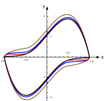
As an example, and to conclude this section, we plot in Fig. 3 the form of the van der Pol limit cycle when y0(x)subscript𝑦0𝑥y_{0}(x), y0(x)+y1(x)subscript𝑦0𝑥subscript𝑦1𝑥y_{0}(x)+y_{1}(x) and y0(x)+y1(x)+y2(x)subscript𝑦0𝑥subscript𝑦1𝑥subscript𝑦2𝑥y_{0}(x)+y_{1}(x)+y_{2}(x) are used as approximated limit cycles. It is not banal to recall here that the reconstruction of the shape of limit cycles is not a problem less difficult than that of the calculation of their amplitudes.

Refer to caption

Figure 3: Approximated shape of the van der Pol limit cycle for ϵ=5italic-ϵ5\epsilon=5 and h(ϵ)italic-ϵh(\epsilon) given in (3.34). Black line: the experimental limit cycle. Brown, blue and red lines: the curves y0(x)subscript𝑦0𝑥y_{0}(x), y0+y1(x)subscript𝑦0subscript𝑦1𝑥y_{0}+y_{1}(x) and y0+y1(x)+y2(x)subscript𝑦0subscript𝑦1𝑥subscript𝑦2𝑥y_{0}+y_{1}(x)+y_{2}(x), respectively.

4 Conclusions

In this work, the conjecture (2.8) has been posed. This is a consequence of the different formulas here presented for approximating the amplitude a𝑎a of the van der Pol limit cycle. In addition to the well known constant approximation a¯=2¯𝑎2\bar{a}=2 that generates an error less than 1%percent11\%, we establish a family of recursive formulas that are valid for the whole range of the parameter ϵitalic-ϵ\epsilon. Two of them, aR1(ϵ)subscript𝑎𝑅1italic-ϵa_{R1}(\epsilon) and aR2(ϵ)subscript𝑎𝑅2italic-ϵa_{R2}(\epsilon), have been explicitly given. The first one, aR1subscript𝑎𝑅1a_{R1}, produces an error less than 0.1%percent0.10.1\% and the second one, aR2subscript𝑎𝑅2a_{R2}, reduces the error to less than 0.05%percent0.050.05\%. Moreover, aR2subscript𝑎𝑅2a_{R2} is conjectured to be an upper bound of a𝑎a.

As far as we know, this is the first time where an analytical approximation of the amplitude of the van der Pol limit cycle, with validity from the weakly up to the strongly nonlinear regime, is proposed.

Acknowledgements:

The Gobierno of Navarra, Spain, Res. 07/05/2008 is acknowledged by its financial support.

References

  • [1] Van der Pol B. On relaxation oscillations. Phil Mag 1926; 2:978–992
  • [2] Andronov AA, Vitt AA, Khaikin SE. Theory of oscillators, Dover, New York; 1989.
  • [3] Van der Pol B and van der Mark M. Le battement du coeur consideré comme oscillation de relaxation et un modèle électrique du coeur (The beating of the heart considered as relaxation oscillation and an electric model of the heart). L’onde électrique 1928; 7:365–392.
  • [4] López-Ruiz R, Pomeau Y. Transition between two oscillation modes. Phys Rev E 1997; 55:R3820-R3823.
  • [5] Odani K. The limit cycle of the van der Pol equation is not algebraic. J Differen Equat 1995; 115:146–152.
  • [6] Jordan AW, Smith P. Nonlinear ordinary differential equations, Oxford University Press, Oxford; 1977.
  • [7] Ye Y. Theory of limit cycles. In: Trans Math Monographs, vol. 66. Boston: American Mathematical Society; 1986.
  • [8] Liao SJ. The proposed homotopy analysis technique for the solutions of non-linear problems, Ph.D. Thesis, Shanghai Jiao Tong University, 1992.
  • [9] Liao SJ. Beyond perturbation: introduction to the homotopy analysis method. Boca Raton: Chapman & Hall/CRC Press; 2003.
  • [10] Liao SJ. An analytic approximate approach for free oscillations of self-excited systems. Int J Non-Linear Mech 2004;39:271–280.
  • [11] Wu W, Liao SJ. Solving solitary waves with discontinuity by means of the homotopy analysis method. Chaos, Solitons & Fractals 2005;26:177–185.
  • [12] Hayat T, Khan M. Homotopy solutions for a generalized second-grade fluid past a porous plate. Nonlinear Dynam 2005;42:395–405.
  • [13] Abbasbandy S. The application of homotopy analysis method to solve a generalized Hirota–Satsuma coupled KdV equation. Phys Lett A 2007;361:478–483.
  • [14] Abbasbandy S. Homotopy analysis method for heat radiation equations. Int Commun Heat Mass Transf 2007;34:380–387.
  • [15] Abbasbandy S, Tan Y, Liao SJ. Newton-Homotopy analysis method for nonlinear equations. Appl Math Comput 2007;188:1794–1800.
  • [16] Tan Y, Abbasbandy S. Homotopy analysis method for quadratic Riccati differential equation. Commun Nonlinear Sci Numer Simul 2008;13:539–546.
  • [17] Abbasbandy S, Lopez JL, Loper-Ruiz R. The homotopy analysis method and the Liénard equation. Arxiv:0805.3916[nlin.PS].
  • [18] Odani K. On the limit cycle of the Liénard equation. Archivum Mathematicum (Brno) 2000;36:25–31.
  • [19] López JL, López-Ruiz R. Approximating the amplitude and form of limit cycles in the weakly nonlinear regime of Liénard systems. Chaos, Solitons & Fractals 2007;34:1307–1317.
  • [20] López JL, López-Ruiz R. The limit cycles of Liénard equations in the weakly nonlinear regime. ArXiv 2006;nlin/0605025.
  • [21] Cartwright ML. Van der Pol’s equation for relaxation oscillation. In Contributions to the theory of non-linear oscillations II, S. Lefschetz ed. Ann. of Math. Studies 1952;29:3–18.
  • [22] López JL, López-Ruiz R. The limit cycles of Liénard equations in the strongly nonlinear regime. Chaos, Solitons & Fractals 2000;11:747 -756.
  • [23] López-Ruiz R, López JL. Bifurcation curves of limit cycles in some Liénard systems. Int J Bifurcat Chaos 2000;10:971-980.
  • [24] Riordan, J. Combinatorial Identities, John Wiley & Sons, New York; 1968.