Bayesian outlier detection in Capital Asset Pricing Model

Abstract

We propose a novel Bayesian optimisation procedure for outlier detection in the Capital Asset Pricing Model. We use a parametric product partition model to robustly estimate the systematic risk of an asset. We assume that the returns follow independent normal distributions and we impose a partition structure on the parameters of interest. The partition structure imposed on the parameters induces a corresponding clustering of the returns. We identify via an optimisation procedure the partition that best separates standard observations from the atypical ones. The methodology is illustrated with reference to a real data set, for which we also provide a microeconomic interpretation of the detected outliers.

Keywords: Capital Asset Pricing Model, Constrained optimisation algorithm, Markov Chain Monte Carlo, Outlier identification, Parametric product partition models, Score function.

1 Introduction

In this paper we propose a novel Bayesian optimisation procedure for outlier identification in a Capital Asset Pricing framework. The Capital Asset Pricing Model (CAPM), see Sharpe (1964), Lintner (1965), Mossin (1966) and Black (1972), states that an asset expected return is equal to the risk free rate plus a prize for risk. The CAPM is widely used in applications to evaluate the performance of assets and portfolios, and different performance measures are based on it, see e.g. chap. 4 in Amenec and Le Sourd (2003). In particular, it is very useful for the calculation of the cost of capital equities, which is necessary for market based firm value models, see e.g. Ross et al. (2008). The CAPM can be represented by a simple linear regression where the slope identifies the systematic risk of an asset, that is it measures the return sensitivity to movement in the market. The systematic risk represents the component of the risk that cannot be eliminated simply via portfolio diversification. Therefore, systematic risk is a key variable to be taken into account for asset allocation and portfolio management.

Almost all empirical analysis of the CAPM has been carried out in the classical framework, see i.e. Fama and French (2004) for an exaustive review. The systematic risk is usually estimated by the least square method which coincides with the maximum likelihood estimator under the assumption of normality. It is well known that this approach has at least two disadvantages. Firstly, this estimation method is sensitive to the presence of outliers, that is observations that do not follow the same statistical model as the main part of the data. Secondly, it is not possible to incorporate prior beliefs about behaviour of returns in the model.

In this paper, to overcome these problems, we focus on Bayesian robust estimation procedures for linear regression models; see e.g. Chaturvedi (1996), Fernández et al. (2001), Quintana and Iglesias (2003) and Quintana et al. (2005a, 2005b). In particular, Quintana and Iglesias (2003) and Quintana et al. (2005a) show that outlying points can be accommodated either by a product partition model with a normal structure on the returns, or by a simple regression model with $t$ shape errors and small degrees of freedom.

We follow the first approach and we apply a normal model with a partition structure on the parameters of interest. This approach has at least two advantages. Firstly, the use of a normal distribution is consistent with the assumption of mean-variance analysis required by CAPM. Secondly, the use of a partition structure simultaneously yields outlier identification and model robustification. The partition structure allows us to separate the main body of “standard” data points from the “atypical” ones.

Regarding the outlier identification problem we work in a Bayesian decision theoretical framework. The partition that best separates “standard” observations from the “atypical” ones is selected by minimising a specific score function. In Quintana and Iglesias (2003) this partition is identified by applying a clustering algorithm. However, as they mentioned (see page 572 in Quintana and Iglesias, 2003), a weakness of their algorithm is that it could be trapped in local modes. Furthermore, as they select outlying points one by one, they could incur in the problem of masking. If a data set has multiple outliers, they may mask one another, making outlier identification difficult. Masked outliers should be removed as a group, otherwise their presence could remain undetected. We overcome these problems by applying a constrained optimisation algorithm to select the optimal partition. Our algorithm includes a preliminary step in which the data are prescreened via a robust technique that allows us to identify a set of potential outliers. Subsequently, outliers are efficiently selected among the potential ones.

The paper is structured as follows. In Section 2 we briefly introduce the CAPM and parametric product partition models (PPM). In Section 3 we describe the optimisation algorithm used for outlier identification. For comparative purposes, in Section 4 we apply our procedure to the IPSA data set, previously examined by Quintana et al. (2005a). Conclusions are given in Section 5.

2 Background and preliminaries

2.1 The CAPM

According to CAPM, the expected return of any asset $i$ is a linear function of the market portfolio one

$$E\left(R_{i}\right)=R_{f}+\beta_{i}\left(E\left(R_{m}\right)-R_{f}\right),\quad i=1,\ldots,N,$$ (2.1)

where $N$ is the number of assets, $R_{i}$ is the return of asset $i$, $R_{f}$ is the risk-free rate of return, $R_{m}$ is the return on the market portfolio and the slope $\beta_{i}$ measures the systematic risk. The market portfolio is the portfolio containing every asset available to the economic agent, in amounts proportional to their total market values. Market portfolio is a theoretical concept, hence it is necessary to use a market index return, $R_{M}$, as an observable proxy of the market portfolio return $R_{m}$.

An extension of equation (2.1) is often used to estimate the systematic risk. Another coefficient denoted by $\alpha_{i}$ is usually introduced, obtaining the following expression

$$E\left(R_{i}\right)-R_{f}=\alpha_{i}+\beta_{i}\left(E\left(R_{M}\right)-R_{f}\right),\quad i=1,\ldots,N,$$ (2.2)

where $\alpha_{i}$ denotes wether the asset $i$ over/under-performs the expected return explained by CAPM. The parameters of equation (2.2) are estimated by using the linear regression equation

$$R_{it}-R_{ft}=\alpha_{i}+\beta_{i}\left(R_{Mt}-R_{ft}\right)+\varepsilon_{it},$$ (2.3)

$$y_{it}=\alpha_{i}+\beta_{i}x_{t}+\varepsilon_{it},\quad i=1,\ldots,N,\quad t=1,\ldots,T,$$

where, for a $t$-period and a generic asset $i$, $y_{it}$ is the excess return of the asset, $R_{it}$ denotes the return of the asset, $R_{ft}$ is the risk-free rate of return, $R_{Mt}$ is the market index return and $\varepsilon_{it}$ is a normally distributed error term.

The estimation of the systematic risk $\beta_{i}$ can be affected by the presence of outlying points. An approach that carefully takes into account the presence of anomalous observations should be applied. In this paper we model outliers by a shift in the regression mean and we handle them working with an extension of equation (2.3). More precisely, we assume that excess returns of share $i$, at different time points $t$, can be more appropriately described by a set of parallel regression lines (see also Quintana and Iglesias, 2003 and Quintana et al., 2005a). We allow $\alpha_{i}$ to change with $t$ (indicated as $\alpha_{it}$), and we estimate the following equation

$$y_{it}=\alpha_{it}+\beta_{i}x_{t}+\varepsilon_{it},\quad i=1,\ldots,N,\quad t=1,\ldots,T,$$ (2.4)

where $\alpha_{it}$ assumes values in the finite set $\boldsymbol{\alpha}_{\rho_{i}}=\left(\alpha^{*}_{i1},\ldots,\alpha^{*}_{i|\rho_{i}|}\right)$, with cardinality $|\rho_{i}|$ smaller then $T$ (more details will be provided in Section 2.2). In fact, it can be realistically assumed that the number of regression lines is inferior to the number of observations. Our aim is to group together (to cluster) time periods with common values of the intercepts. These groups lead to a clustering of the corresponding excess returns $y_{it}$. We will end up with a main group of standard observations and one or more groups of atypical ones. The number and the composition of the groups (the partition structure) is unknown, hence we assign a prior distribution to the set of all possible partitions, see Section 2.2 for the details.

2.2 A parametric product partition model

Following Quintana and Iglesias (2003) and Quintana et al. (2005a), we use a parametric product partition model (PPM) to robustly estimate the systematic risk and to identify outlying points. We now briefly review the theory on parametric product partition models with reference to our specific problem, see Barry and Hartigan (1992) for a detailed and more general presentation.

Given the model described by equation (2.4), let $S_{i}^{0}=\{1,\ldots,T\}$ be the set of time periods. A partition of the set $S_{i}^{0}$, $\rho_{i}=\left\{S_{i}^{1},\ldots,S_{i}^{d},\ldots,S_{i}^{|\rho_{i}|}\right\}$ with cardinality $|\rho_{i}|$, is defined by the property that $S_{i}^{d}\cap S_{i}^{d^{\prime}}=\emptyset$ for $d\neq d^{\prime}$ and $\cup_{d}\,S_{i}^{d}=S_{i}^{0}$. The generic element of $\rho_{i}$ is $S_{i}^{d}=\left\{t:\alpha_{it}=\alpha^{*}_{id}\right\}$, where $\boldsymbol{\alpha}_{\rho_{i}}=\left(\alpha^{*}_{i1},\ldots,\alpha^{*}_{i|\rho_{i}|}\right)$ is the vector of the unique values of $\boldsymbol{\alpha}_{i}=\left(\alpha_{i1},\ldots,\alpha_{iT}\right)$. All $\alpha_{it}$ whose subscripts $t$ belong to the same set $S_{i}^{d}\in\rho_{i}$ are (stochastically) equal; in this sense they are regarded as a single cluster.

We assign to each partition $\rho_{i}$ the following prior probability

$$P\left(\rho_{i}=\left\{S_{i}^{1},\ldots,S_{i}^{|\rho_{i}|}\right\}\right)=K\prod_{d=1}^{|\rho_{i}|}C\left(S_{i}^{d}\right),$$ (2.5)

where $C\left(S_{i}^{d}\right)$ is a cohesion function and $K$ is the normalising constant. Equation (2.5) is referred to as the product distribution for partitions. The cohesions represent prior weights on group formation and formalise our opinion on how tightly clustered the elements of $S_{i}^{d}$ would be.

The cohesions can be specified in different ways, a useful choice is

$$C\left(S_{i}^{d}\right)=c\times\left(\left|S_{i}^{d}\right|-1\right)!,\quad\quad d=1,\ldots,|\rho_{i}|$$ (2.6)

for some positive constant $c$.

For moderate values of $c$, e.g. $c=1$, the cohesions in (2.6) yield a prior distribution that favours the formation of partitions with a reduced number of large subsets. This is a desirable feature for an outlier detection model, since we do not want to identify too many subsets of points as outliers. For more details on the choice of $c$ see i.e.  Liu (1996), Quintana et al. (2005b) and Tarantola et al. (2008).

Moreover, there is an interesting connection between parametric PPMs and the class of Bayesian nonparametric models based on a mixture of Dirichlet Processes (Antoniak, 1974). Under the latter prior, the marginal distribution of the observables is a specific PPM with the cohesion functions specified by equation (2.6), see Quintana and Iglesias (2003). This connection allows us to use efficient Markov Chain Monte Carlo (MCMC) algorithms developed for Bayesian nonparametric problems like the one that we apply here.

In this paper we consider the following Bayesian hierarchical model

$$y_{it}|\rho_{i},\left(\alpha^{*}_{i1},\ldots,\alpha^{*}_{i|\rho_{i}|}\right),\beta_{i},\sigma_{i}^{2}\overset{ind}{\sim}N\left(\alpha_{it}+\beta_{i}x_{t},\sigma_{i}^{2}\right)$$

$$\alpha^{*}_{i1},\ldots,\alpha^{*}_{i|\rho_{i}|}|\rho_{i},\sigma_{i}^{2}\overset{IID}{\sim}N\left(a,\tau_{0}^{2}\sigma_{i}^{2}\right)$$

$$\beta_{i}|\sigma_{i}^{2}\sim N\left(b,\gamma_{0}^{2}\sigma_{i}^{2}\right)$$

$$\rho_{i}\sim\mbox{product distribution,}\;\mbox{with}\;C\left(S_{i}^{d}\right)=c\times\left(\left|S_{i}^{d}\right|-1\right)!$$

$$\sigma_{i}^{2}\sim IG(v_{0},\lambda_{0}),$$

where $a$, $b$, $\tau^{2}_{0}$, $\gamma^{2}_{0}$, $v_{0}$ and $\lambda_{0}$ are user-specified hyperparameters, the product distribution is defined in (2.5) and $IG\left(v_{0},\lambda_{0}\right)$ is an inverted gamma distribution with $E\left(\sigma_{i}^{2}\right)=\lambda_{0}/\left(v_{0}-1\right)$. The Gibbs algorithm applied to sample from the posterior distributions of the parameters is described in the Appendix.

3 Optimal outlier detection

To detect outlying points we apply a constrained optimisation algorithm, working in a Bayesian decision theoretic framework. Our aim is to select the partition that best separates the main group of standard observations from one or more groups of atypical data. Each partition corresponds to a different model and the best model is the one minimising a given loss function. We consider a loss function that combines the estimation of the parameters and the partition selection problems.

Given a generic asset $i$, let $\left(\boldsymbol{\alpha}_{i},\beta_{i},\sigma^{2}_{i}\right)$ be the vector of parameters of the model and $\left(\boldsymbol{\alpha}_{\rho_{i}},\beta_{\rho_{i}},\sigma^{2}_{\rho_{i}}\right)$ be the corresponding vector that results when fixing $\rho_{i}$. We consider the loss function

$$L\left(\rho_{i},\boldsymbol{\alpha}_{\rho_{i}},\beta_{\rho_{i}},\sigma^{2}_{\rho_{i}},\boldsymbol{\alpha}_{i},\beta_{i},\sigma^{2}_{i}\right)=\frac{k_{1}}{T}\ \parallel\boldsymbol{\alpha}_{\rho_{i}}-\boldsymbol{\alpha}_{i}\parallel^{2}\ +\ k_{2}\ \left(\beta_{\rho_{i}}-\beta_{i}\right)^{2}\ +$$

$$+k_{3}\ \left(\sigma^{2}_{\rho_{i}}-\sigma_{i}^{2}\right)^{2}\ +\ \left(1-k_{1}-k_{2}-k_{3}\right)|\rho_{i}|,$$ (3.1)

where $\parallel\cdot\parallel$ is the Euclidean norm, and $k_{j}$ ($j=1,2,3$) are positive cost-complexity parameters with $\sum_{j=1}^{3}k_{j}\leq 1$. Minimizing the expected value of (3.1) is equivalent to choosing the partition that minimises the following score function

$$SC\left(\rho_{i}\right)=\frac{k_{1}}{T}\ \parallel\hat{\boldsymbol{\alpha}}_{i}^{B}(y)-\hat{\boldsymbol{\alpha}}_{\rho_{i}}(y)\parallel^{2}\ +\ k_{2}\ \left[\hat{\beta}_{i}^{B}(y)-\hat{\beta}_{\rho_{i}}(y)\right]^{2}\ +$$

$$+k_{3}\ \left[\big{(}\hat{\sigma}^{B}_{i}(y)\big{)}^{2}-\hat{\sigma}_{\rho_{i}}^{2}(y)\right]^{2}\ +\ \left(1-k_{1}-k_{2}-k_{3}\right)|\rho_{i}|.$$ (3.2)

In (3.2), a superscript “$B$” means that we consider the Bayesian estimates of the corresponding parameter, whereas a subscript “$\rho_{i}$” denotes the estimate of the parameter (or vector of parameters) conditionally on the partition $\rho_{i}$. Formally, if we indicate with $\theta$ a generic parameter in (3.2), we get $\hat{\theta}^{B}(y)=E(\theta|y)$ and $\hat{\theta}_{\rho_{i}}(y)=E(\theta|y,\rho_{i})$. The estimates $\hat{\theta}^{B}(y)$ and $\hat{\theta}_{\rho_{i}}(y)$ of $\theta$ are obtained via the MCMC method described in the Appendix.

The number of all possible partitions is equal to $B(a)$, the Bell number of order $a$, recursively defined by $B(a+1)=\sum_{k=0}^{a}\binom{a}{k}B(k)$, with $B(0)=1$. This quantity is extremely large even for moderate values of $a$, therefore we need to restrict our search to a tractable subset of all partitions.

To avoid evaluating and comparing the scores of an impossibly large number of partitions, we propose a two step algorithm. This algorithm reduces by construction the probability of incurring the masking problem. It examines all partitions having a given structure, and groups of observations may be included/excluded as block in the different clusters.

In the first step of the algorithm we use least trimmed squares (LTS) regression, see Rousseeuw (1984) and Rousseeuw and Leroy (1987), to prescreen the data and identify a large set of potential outliers. A similar idea has been successfully applied by Hoeting et al. (1996) for simultaneous variable selection and outlier identification in a linear regression model. LTS is also used in the Bayesian Model Averaging Package of R (Raftery et al.,  2008) to prescreen the data.

In the second step, we constrain our search to partitions identifying as outliers only particular subsets of those identified by LTS, and we select the one that minimises the score function (3.2).

Among robust techniques, we have chosen LTS since it has a very high (finite-sample) breakdown point (close to $1/2$) and tends to identify a large number of observations as abnormal, reducing the possibility of misclassifying anomalous points. However, it should be noticed that LTS can be rather sensitive to small perturbations in the central part of the data (high subsample sensitivity), see e.g. Ellis (1998), Víšek (1999), and Čížek and Víšek (2000). Attention should be paid to check if the set of potential outliers is reasonable. In the specific case examined here the set of potential outliers is sensible. In fact the elements selected by LTS correspond to “small/high” values of the components $\widehat{\boldsymbol{\alpha}}^{B}_{i}(y)$.

The algorithm consists of the following two steps. Let $i$ be a generic asset.

• We apply LTS to the excess returns of the asset $i$. All points with an absolute value of the standardized residuals greater than $2.5$ are considered as potential outliers.

• Let $\mathcal{O}^{LTS}_{i}$ be the set of all time points corresponding to the potential outliers identified in Step 1. We restrict our search to partitions with cardinality $2$ or $3$ where the outliers are particular subsets of $\mathcal{O}^{LTS}_{i}$.

  The data are classified in clusters $S_{i}^{1}$, $S_{i}^{2}$ and $S_{i}^{3}$ defined as follows. Cluster $S_{i}^{2}$ contains “standard observations”, with $\left(S^{0}_{i}\setminus O_{i}^{LTS}\right)\subseteq S_{i}^{2}$. The remaining data, identifying “anomalous points”, are classified either in $S_{i}^{1}$ (“anomalous low values”) or in $S_{i}^{3}$ (“anomalous high values”) with $\left(S_{i}^{1}\cup S_{i}^{3}\right)\subseteq O_{i}^{LTS}$.

  We only consider partitions with the following alternative structures $\rho_{i}=\left\{S_{i}^{1},S_{i}^{2},S_{i}^{3}\right\}$ or $\rho_{i}=\left\{S_{i}^{2},\left(S_{i}^{1}\cup S_{i}^{3}\right)\right\}$. If a cluster is empty it is not considered as a component of $\rho_{i}$. We do not consider the case in which both $S_{i}^{1}$ and $S_{i}^{3}$ are empty.

  The methodology used to construct the clusters $S_{i}^{1}$, $S_{i}^{2}$ and $S_{i}^{3}$ is described below.

  • Given the vector $\widehat{\boldsymbol{\alpha}}^{B}_{i}(y)=\left(\widehat{{\alpha}}^{B}_{i_{1}},\ldots,\widehat{{\alpha}}^{B}_{i_{T}}\right)$ of the Bayesian estimates of the intercepts of model (2.4), we indicate with $me$ the median of its elements.

  • For each time point $\ell\in\mathcal{O}^{LTS}_{i}$ we compute the deviation from the median, $d_{\ell}=\left(\widehat{{\alpha}}^{B}_{i_{\ell}}-me\right)$.

  • We construct the set $\mathcal{D}$ containing all deviations from the median and two instrumental extra points

    $$\mathcal{D}=\left\{\left\{d_{\ell},\;\;\ell\in\mathcal{O}^{LTS}_{i}\right\}\bigcup\left\{\min\limits_{\ell}\left(d_{\ell}\right)-\kappa,\ \max\limits_{\ell}\left(d_{\ell}\right)+\kappa\right\}\right\},$$

    with $\kappa>0$ such that $\min\limits_{\ell}\left(d_{\ell}\right)-\kappa<0$ and ${\max\limits_{\ell}\left(d_{\ell}\right)}+\kappa>0.$

  • For every possible couple of values $\left(d^{L},d^{U}\right)\in\left(\mathcal{D}\times\mathcal{D}\right)$, with $d^{L}<0$ and $0\leq d^{U}$, we classify in $S_{i}^{1}$ all $\ell\in\mathcal{O}^{LTS}_{i}$ such that $d_{\ell}\leq d^{L}$ and in $S_{i}^{3}$ all $\ell\in\mathcal{O}^{LTS}_{i}$ that $d_{\ell}\geq d^{U}$, that is $S_{i}^{1}=\left\{\ell\in\mathcal{O}^{LTS}_{i}:d_{\ell}\leq d^{L}\right\}$ and $S_{i}^{3}=\left\{\ell\in\mathcal{O}^{LTS}_{i}:d_{\ell}\geq d^{U}\right\}$. The remaining points are classified in $S_{i}^{2}$.

    In this way we construct a list of possible partitions, that will then be compared in terms of the value of the score function (3.2). The optimal partition is the one with the minimum score function value.

4 Analysis of the IPSA stock market data

To test the performance of our procedure we analysed the IPSA stock market data, previously examined by Quintana et al. (2005a). The IPSA is the main index of the “Bolsa de Comercio de Santiago” (Santiago Stock Exchange). It corresponds to a portfolio containing the 40 most heavily traded stocks, the list is revised quarterly.

We considered monthly data relative to the period January 1990-June 2004. We used the IPSA index as a proxy of the Chilean market portfolio and the interest rate of Central Bank discount bonds as the risk free rate. We focused our analysis only on the 5 shares listed in Table 1, for which Quintana et al. (2005a) provided a detailed analysis both of the estimates of the parameters and of the selected partitions.

We used the following values of the hyperparameters $c=1$, $a=0$, $b=1$, $\tau_{0}^{2}=\gamma_{0}^{2}=1000$, $v_{0}=2.0001$, $\lambda_{0}=0.010001$. We set $\left(k_{1},k_{2},k_{3}\right)=\frac{1}{2012}(1000,1000,1)$ in (3.1) and (3.2), to give priority to the estimation of $\boldsymbol{\alpha}_{i}$ and $\beta_{i}$, imposing weak restriction on the number of clusters. These values lead to the same prior distributions and the same relative weights for the score function components as in Quintana et al. (2005a).

The two MCMC algorithms, used respectively to obtain the Bayesian estimates of the parameters and the estimates given a specific partition, are both based on a run of $10\thinspace 000$ sweeps with a burn-in of $1\thinspace 000$ iterations. Convergence of the MCMC was assessed using standard criteria, see e.g. Best et al. (1995) and Cowles and Carlin (1996). No specific indication of abnormal behaviour is obtained. The two MCMC algorithms required 16 and 2.9 minutes respectively per $10\thinspace 000$ iterations on a Pentium IV 3.4 GHz, 1 GB RAM personal computer. The programs were written in MATLAB; it is expected that a lower level programming language could speed up the execution time by a factor of at least $5$.

4.1 Numerical results

In Table 1 we report the partitions selected by our algorithm and the one proposed by Quintana et al. (2005a), denoted by DMT and QIB respectively. The MCMC standard errors of the estimates were calculated by splitting the Markov chain output into batches, see Geyer (1992). It is also indicated the value of the score function $SC$ and of the proportional reduction in score ($PRS$), that is $PRS=(\mathrm{SC}_{\mathrm{QIB}}-\mathrm{SC}_{\mathrm{DMT}})/\mathrm{SC}_{\mathrm{QIB}}$; for all shares $SC_{DMT}\leq SC_{QIB}$. The PRS is large for $3$ out of $5$ cases (more than $33\%$), in particular it is equal to $61.97\%$ for the Concha y Toro share.

TABLE 1 ABOUT HERE

Note that for the Concha y Toro and Entel shares the outliers selected by Quintana et al. (2005a) are a subset of those identified with our procedure. For the Cementos Bío Bío S.A. and Copec S.A. we select the same outlier set, but since we group them in only one cluster we obtain a lower value of the score function.

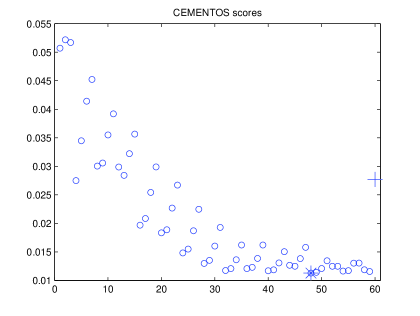
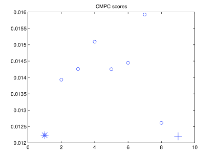
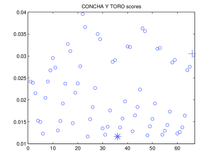
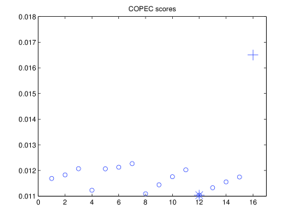
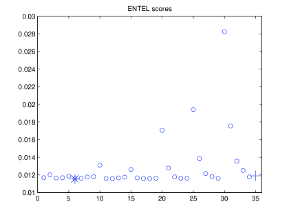
Figure 1 reports the scores of all partitions explored by our algorithm and the score of the partition selected by Quintana et al. (2005a). For the Cementos, Concha y Toro and Copec shares many partitions, explored by our algorithm, present a lower value of the score function than the one selected by Quintana et al. (2005a).

FIGURE 1 ABOUT HERE

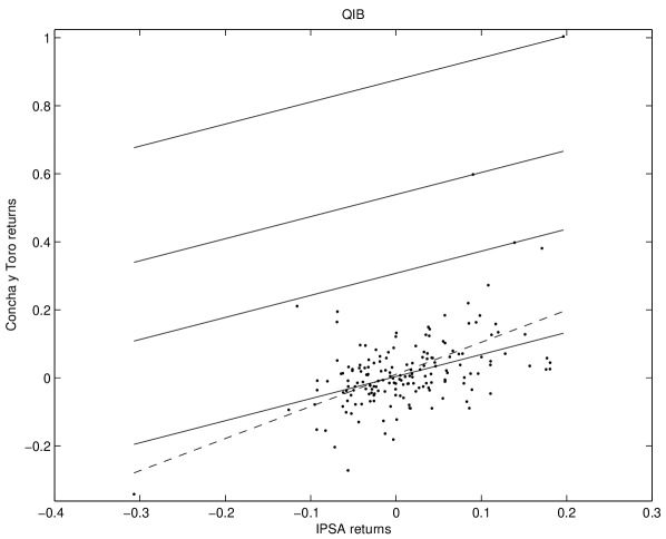
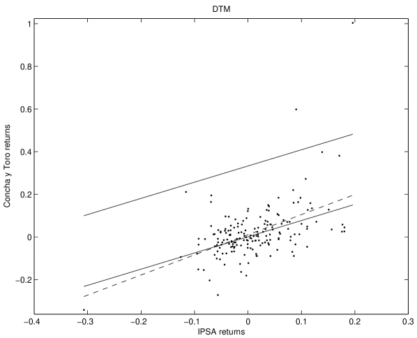
A more detailed analysis of the Concha y Toro share is provided in Figure 2 and Table 2. In Figure 2 we represent the Bayesian linear regression lines obtained applying the algorithm by Quintana et al. (2005a) and the one proposed here. The best partition of Quintana et al. (2005a) produces a regression line for each detected outlier. In Table 2 we report the Bayesian estimates of the systematic risk under the three different partition structures considered in Figure 2.

FIGURE 2 ABOUT HERE

TABLE 2 ABOUT HERE

In Table 3 we report, with reference to the Concha y Toro data, a sensitivity analysis of the results for different choices of the constant $c$ in (2.6). Note that, for a wide range of values of $c$ our results are remarkably robust.

TABLE 3 ABOUT HERE

4.2 Microeconomic analysis

We performed a microeconomic analysis of the companies under study, and we list some events that could have produced the abnormal behaviour identified by the outliers. All the information provided is freely available on the World Wide Web.

1) CEMENTOS BÍO-BÍO S.A.  The Cementos Bío Bío S.A. is a company involved in the production and sale of cement and lime products, wood and its by-products, premixed concrete and ceramics.

In 1992 (outlier 27) it opened a new cement plant in Copiapo.

In 1998 (outlier 107) it expanded the cement plant in Antofagasta and started up a new cement plant in Curicó.

In 1999 (outliers 112, 113) Cementos de Mexico, the world’s third-largest cement manufacturer, entered the Chilean market by acquiring 12% of the Cementos Bío Bío S.A. shares.

2) CMPC  The group’s principal activity is manufacturing pulp and paper in Chile. It is an integrated company that undertakes its industrial work through five business affiliates (CMPC Celulosa, CMPC Papeles, CMPC Productos de Papel, CMPC Tissue, and Forestal Mininco), and owns industrial plants in Chile, Argentina, Peru and Uruguay.

The years from 1990 to 1992 (outlier 15) were characterised by an expansion in Latin America. In 1990 CMPC entered Argentina by purchasing (in partnership with Procter & Gamble), Quimica Estrella San Luis S.A. (now Prodesa), a manufacturer of sanitary napkins and paper diapers. In 1992 CMPC formed a strategic alliance with Procter & Gamble to develop markets for the aforementioned products in Chile, Argentina, Bolivia, Paraguay, Peru, and Uruguay.

3) CONCHA Y TORO  Concha y Toro is one of the leading producers of wine in Chile. It produces and exports a wide range of wines. In 1994, Concha y Toro became the first Chilean winery to be listed on the New York Stock Exchange.

During the years 1991-1993 (outliers 14, 18, 21, 22, 27) important changes took place. Concha y Toro tripled the size of its vineyards to reduce dependence on outside grape growers and enrolled the help of French and Californian oenologists. It modernized its production and transformed the original Concha y Toro mansion into the head quarters of the firm for its export operations.

In 1996 Concha y Toro purchased a vineyard in the Mendoza region in Argentina. In 1997 the company and the French firm Baron Philippe de Rothschild S.A. endorsed a joint venture with the aim of producing a wine to the standards of the French Grand Cru Class . In 1998 (outlier 97) Concha y Toro launched Vina Almaviva into the market. In the same year the company ranked second among wine exporters to the United States.

4) COPEC S.A.   Copec S.A. is a diversified Chilean financial holding company that participates through subsidiaries and related companies in different business sectors (energy, forestry, fishing, mining and power industries).

In 1992 (outlier 31) it united two fisheries to form Igemar that became the biggest fishing and fish-processing company in Chile.

In 1998 (outlier 107) it became Chile’s largest exporter outside of the mining sector.

In 1999 (outlier 111) COPEC created Air Bp Copec S.A. to commercialise fuels for national and international air lines, in joint venture with BP Global Investments.

5) ENTEL  Entel was created in 1964 as a state company, and it was privatised in 1986. The group’s principal activities are providing telecommunication services. It also operates in Central America and Peru aside from its centre of major operations which is located in Chile.

In 1996 (oulier 65) Telecom Italia acquired a $19.99\%$ of Entel shares.

5 Concluding remarks

In this paper we presented a model for robust inference in CAPM in the presence of outliers. Working in a Bayesian decision framework, we developed a constrained optimization algorithm for outlier detection. Differently from the methodology proposed by Quintana et al. (2005a) it appeared to be successful in the identification of masked outliers and led to partitions with a lower value of the score function.

The outlier identification procedure proposed by Quintana and Iglesias (2003) is based on a hierarchical divisive method. Their procedure works by detaching, one by one, the most outlying component from the vector $\hat{\boldsymbol{\alpha}}_{i}^{B}(y)$ of the Bayesian estimates. This procedure is irreversible, that is once a point is classified in a specific cluster it is not taken any more under consideration. On the other hand our algorithm allow groups of observations to be considered simultaneously as potential outliers. This could be a possible explanation of why in some cases, as for the Concha y Toro share, the algorithm by Quintana and Inglesias (2003) identifies a smaller set of outliers, incurring in the the masking problem.

A microeconomic analysis is provided to confirm that the selected outlying points are linked to extraordinary events in the history of the examined companies.

Appendix: A Gibbs sampling algorithm

We adapt to our problem a Gibbs sampling algorithm, proposed by Bush and MacEachern (1996). Consider a generic asset $i$. Given the starting values $\alpha_{0},\ \beta_{0}$ and $\sigma^{2}_{0}$ we iteratively sample from the following distributions

$$\beta_{i}|\sigma_{i}^{2},\boldsymbol{\alpha}_{i},\mathbf{y}_{i}\sim N\left\{\frac{b/\gamma_{0}^{2}+\sum_{t=1}^{T}(y_{i_{t}}-\alpha_{i_{t}})x_{t}}{1/\gamma^{2}_{0}+\sum_{t=1}^{T}x_{t}^{2}},\frac{\sigma_{i}^{2}}{1/\gamma^{2}_{0}+\sum_{t=1}^{T}x_{t}^{2}}\right\}\;\;$$

$$\sigma_{i}^{2}|\boldsymbol{\alpha}_{i},\beta_{i},\boldsymbol{y}_{i}\sim IG\left\{v_{0}+\frac{T+|\rho_{i}|+1}{2},\lambda_{0}+\frac{(\beta_{i}-b)^{2}}{2\gamma_{0}^{2}}+\frac{1}{2\tau_{0}^{2}}\sum^{|\rho_{i}|}_{d=1}(\alpha^{*}_{i_{d}}-a)^{2}\right.$$

$$\;\;\;\;\;\;\;\;\;\;\;\;\left.+\frac{1}{2}\sum_{t=1}^{T}(y_{i_{t}}-\alpha_{i_{t}}-\beta x_{t})^{2}\right\}\;\;$$

$$\alpha_{i_{t}}|\boldsymbol{\alpha}_{i_{-t}},\beta_{i},\sigma_{i}^{2},\boldsymbol{y}\propto\sum_{j\neq t}\exp\left\{-\frac{1}{2\sigma^{2}}(y_{i_{t}}-\alpha_{i_{j}}-\beta_{i}x_{t})^{2}\right\}\delta_{\alpha_{i_{j}}}(\alpha_{i_{t}})$$

$$\;\;\;\;\;\;\;\;\;\;\;\;+\frac{\exp\left\{-(y_{i_{t}}-\beta x_{t}-a)^{2}/2\sigma_{i}^{2}(1+\tau_{0}^{2})\right\}}{\sqrt{1+\tau_{0}^{2}}}\;\;N\left(\frac{y_{i_{t}}-\beta_{i}x_{t}+a/\tau_{0}^{2}}{1+1/\tau_{0}^{2}},\frac{\sigma_{i}^{2}}{1+1/\tau_{0}^{2}}\right)$$

where $\boldsymbol{\alpha}_{i_{-t}}=(\alpha_{i_{1}},\ldots,\alpha_{i_{t-1}},\alpha_{i_{t+1}},\ldots,\alpha_{i_{T}})^{\prime}$ and $\delta_{\alpha_{j}}(\cdot)$ is the Kronecker delta function.

Note that $\beta_{i}$ and $\sigma_{i}^{2}$ are sampled from the corresponding full conditional whereas each $\alpha_{i_{t}}$ is sampled from a mixture of point masses and a normal distribution. In this way we automatically update both the vector $\boldsymbol{\alpha}_{i}$ and the partition structure.

Before proceeding to the next Gibbs iteration, we update the vector $\boldsymbol{\alpha}_{i}$ given the partition $\rho_{i}$ sampling from

$$\alpha^{*}_{i_{d}}\sim N\left(\frac{\sum_{t\in S_{d}}(y_{i_{t}}-\beta_{i}x_{t})+a/\tau_{0}^{2}}{|S_{d}|+1/\tau_{0}^{2}},\frac{\sigma_{i}^{2}}{|S_{d}|+1/\tau_{0}^{2}}\right)\;\;\;d=1,\ldots,|\rho_{i}|.$$ (5.3)

This last step was introduced in Bush and MacEachern (1996) to avoid being trapped in sticky patches in the Markov Space.

If the partition structure $\rho_{i}$ is fixed $\beta_{i}$, $\sigma_{i}^{2}$ and $\boldsymbol{\alpha}_{i}$ are directly sampled from the corresponding full conditional distributions, (Appendix: A Gibbs sampling algorithm), in (Appendix: A Gibbs sampling algorithm) and (5.3) respectively.

Table 1: IPSA stock market data: comparison of the results obtained via LTS, QIB’s algorithm (Quintana et al., 2005a) and DMT’s algorithm (De Giuli, Maggi and Tarantola). The second, third and fourth columns display the clustering structure of the outliers. The last three columns show the scores of the partitions selected by Quintana et al. (2005a) and De Giuli, Maggi and Tarantola and production reduction in score (PRS). Figures in brackets are Monte Carlo standard errors $\times 10^{6}.$

Society	$\mathrm{LTS}$	QIB	DMT	$\mathrm{SC}_{\mathrm{QIB}}$	$\mathrm{SC}_{\mathrm{DMT}}$	PRS
CEMENTOS	$\{12,14,18,19,21,27,37,47,59,88,$	$\{12,18,27,37,112,121\},$	$\{12,18,21,27,37,47,59,$	0.0277 (4.79)	0.0113 (4.59)	0.4115
BÍO-BÍO S.A.	$91,107,112,113,121,133,161\}$	{21, 113},$\{47,59,133\},\{107\}$	$107,112,113,121,133\}$
CMPC	$\{3,15,49,50,54,57,100,112\}$	$\{15\}$	$\{15\}$	0.0122 (45.09)	0.0122 (45.09)	0.0000
CONCHA Y	$\{12,14,18,21,22,23,27,29,32,83,$	$\{14\},\{21\},\{27\}$	$\{14,18,21,22,27,97\}$	0.0305 (5.44)	0.0116 (12.57)	0.6197
TORO	$97,104,106,110,144\}$
COPEC S.A.	$\{31,105,107,108,109,111\}$	$\{31,107\},\{111\}$	$\{31,107,111\}$	0.0165 (13.45)	0.0110 (12.27)	0.3333
ENTEL	$\{14,27,29,48,59,63,65,106,111,112\}$	$\{65\}$	$\{59,65\}$	0.0119 (41.73)	0.0116 (54.26)	0.0252

Table 2: Concha y Toro: Bayesian Estimates of the systematic risk obtained with only one cluster, with the partition structure of QI, and with the partition struture of DMT respectively. Figures in brackets are Monte Carlo standard errors $\times 10^{5}.$

Partition structure	$\hat{\beta}^{B}$
$S^{0}$	0.9430 (9.2638)
QIB	0.6486 (7.4916)
DMT	0.7590 (9.0300)

Table 3: Concha y Toro: Sensitivity analysis

$c$ in equation (2.6)	Outliers
$0.01$, $1$ and $5$	$\{14,18,21,22,27,97\}$
$10$ and $50$	$\{14,21,27,97\}$

Figure 1: Score values for the different partition explored by the algorithm of DMT. The optimal value is indicated by a star. A cross represents the partition selected by QIB.

Figure 2: Concha y Toro: Bayesian linear regression lines. The dashed line represents the regression line obtained considering only one cluster. Continuous lines are the Bayesian regression lines for each cluster identified by QIB (first row) and DMT (second row).