1–10
Fine-scale statistics of temperature and its derivatives in convective turbulence
Abstract
We study the fine-scale statistics of temperature and its derivatives in turbulent Rayleigh-Bénard convection. Direct numerical simulations are carried out in a cylindrical cell with unit aspect ratio filled with a fluid with Prandtl number equal to 0.7 for Rayleigh numbers between and . The probability density function of the temperature or its fluctuations is found to be always non-Gaussian. The asymmetry and strength of deviations from the Gaussian distribution are quantified as a function of the cell height. The deviations of the temperature fluctuations from the local isotropy, as measured by the skewness of the vertical derivative of the temperature fluctuations, decrease in the bulk, but increase in the thermal boundary layer for growing Rayleigh number, respectively. Similar to the passive scalar mixing, the probability density function of the thermal dissipation rate deviates significantly from a log-normal distribution. The distribution is fitted well by a stretched exponential form. The tails become more extended with increasing Rayleigh number which displays an increasing degree of small-scale intermittency of the thermal dissipation field for both the bulk and the thermal boundary layer. We find that the thermal dissipation rate due to the temperature fluctuations is not only dominant in the bulk of the convection cell, but also yields a significant contribution to the total thermal dissipation in the thermal boundary layer. This is in contrast to the ansatz used in scaling theories and can explain the differences in the scaling of the total thermal dissipation rate with respect to the Rayleigh number.
1 Introduction
Convective turbulence which is driven by the action of buoyancy forces appears in a wide range of geophysical and astrophysical systems as well as in numerous technological applications such as chip cooling devices or indoor ventilation systems (Kadanoff 2001). The main focus of convection experiments has been on the precise quantification of the global turbulent heat transport through the cell which is measured by the dimensionless Nusselt number as a function of the applied outer temperature difference, the properties of the working fluid and the geometry (see e.g. Niemela & Sreenivasan 2003; Funfschilling et al. 2005). The three dependencies are quantified by dimensionless outer parameters, the Rayleigh number , the Prandtl number and the aspect ratio . The numbers are defined as
| (1) |
where is the thermal expansion coefficient, the gravitational acceleration, the outer temperature difference, the height of the cell and its diameter. The Prandtl number compares the kinematic viscosity of the fluid to the thermal diffusivity of the temperature field. The experiments were able to explore a large range of Rayleigh numbers in the so-called hard turbulence regime from up to in the case of liquid helium (Niemela et al. 2000). However, most experiments can provide pointwise measurements of time series of the turbulent fields only (see e.g. du Puits et al. 2007 and references therein). Only recently, two-dimensional cuts through the flow field have been analysed by combining particle image velocimetry and shadowgraph techniques (Xi, Lam & Xia 2004).
In contrast, direct numerical simulations (DNS) are currently unable to reach in the very high Rayleigh number regime, in particular for aspect ratios . The advantage of DNS is however the fully resolved spatial and temporal information on the turbulent fields and local mechanisms of heat transfer (Kerr 1996; Verzicco & Camussi 2003; Hartlep, Tilgner & Busse 2005; Shishkina & Wagner 2006; Shishkina & Wagner 2007).
Directly related to the Nusselt number is the mean of the thermal dissipation rate which is given by (e.g. Grossmann & Lohse 2000)
| (2) |
The thermal dissipation rate field itself measures the magnitude of the temperature gradient and is defined as
| (3) |
Here, is the three-dimensional position vector and or . Both equations, (2) and (3), imply that the statistics of the fluctuating thermal dissipation field is connected with the local fluctuations of the conductive heat transfer, as given by the local currents, . The measurement of the thermal dissipation field –and thus of spatial derivatives– is experimentally challenging, especially in high-Rayleigh number turbulence. Experiments can usually provide well-resolved time derivatives (Belmonte & Libchaber 1996) or temporal increments of the temperature field (Zhou & Xia 2002). In case of temporal increments in convection, closed forms of the corresponding probability density functions (PDF) of stretched exponential type have been constructed successfully by Ching (1991, 1993). For other flows, such as axisymmetry jets, turbulent channel flows or homogeneous isotropic turbulence, PDFs of the velocity increments have been constructed as a superposition of Gaussian distributions (Castaing et al. 1990) or a product of a Gaussian random variable and a scale-dependent random multiplier (Chevillard et al. 2006). In Rayleigh-Bénard convection, time derivatives however cannot be translated into spatial derivatives by a Taylor frozen-flow hypothesis as in pipe or channel flows. Furthermore, for turbulence in a closed vessel, the concept of homogeneity is limited to the cell centre only. He, Tong & Xia (2007) were recently able to measure four temperature signals close to each other simultaneously to reconstruct temperature gradients. Their analysis disentangled contributions to the total thermal dissipation coming from the bulk and boundary layers. Rayleigh numbers were attained in the experiments, but the resolution of the gradients remained limited to scales larger or equal to the thermal boundary layer thickness. Direct numerical simulations by Kerr (1996) and more recently by Shishkina & Wagner (2007) focused on the geometric properties of thermal plumes, the structures that carry the heat away from the bottom plate.
A detailed statistical analysis of the spatial derivatives of the temperature and the thermal dissipation field in different regions of the convection cell is thus still missing. In particular, knowledge about the strength of the fluctuations around the mean temperature gradient and their dependence on the Rayleigh number allows for a validation of predictions by scaling theories, e.g. those by Grossmann & Lohse (2000). Such analysis is also interesting from the perspective of passive scalar mixing in turbulence where progress in the understanding of the mechanisms that cause intermittent fluctuations has been made recently (Shraiman & Siggia 2000). A first and open point is to understand the differences between passive and active scalars such as the temperature in convective turbulence. For the passive scalar case, it is known that larger amplitudes of the dissipation fields are mostly concentrated on fine scales (Kushnir, Schumacher & Brandt 2006) and that their statistical study puts rather large resolution constraints on DNS. This was discussed by Schumacher, Sreenivasan & Yeung (2005) and Schumacher & Sreenivasan (2005).
In the present work, we provide a detailed height-dependent statistical analysis of the temperature, its fluctuations and spatial derivatives. Odd-order moments of spatial derivatives along an imposed outer mean scalar gradient have been used successfully to quantify deviations from local isotropy in shear flows or for the mixing of scalars in turbulence (Warhaft 2002; Pumir 1996; Schumacher & Sreenivasan 2003). We adopt these ideas for the present active scalar case and discuss the dependence of these anisotropy measures on and in different regions of the convection cell. Finally, we study the statistics of the thermal dissipation rate in the bulk and close to the bottom and top plates of the cell. The results are then related to findings from the passive scalar dissipation field. Our study is intended to build a bridge between the mixing of passive and active scalar fields by comparing the statistical properties for both cases. The outline of this paper is as follows. In the next section, we present the equations of motion and details of the numerical model. The third section discusses the statistics of the total temperature, temperature fluctuations and their gradients. The fourth chapter is on the statistics and Rayleigh number dependence of the thermal dissipation field. Concluding remarks are given at the end.
2 Equations of motion and numerical model
The equations for an incompressible three-dimensional Navier–Stokes fluid in the Boussinesq approximation are solved in combination with the advection–diffusion equation for the temperature field. The system is given by
| (4) | |||||
| (5) | |||||
| (6) |
where is the pressure, the velocity field and the total temperature field. The latter can be decomposed into a mean profile and fluctuations ,
| (7) |
Two different types of statistical averages are used. The average is taken over the whole cell volume and a sequence of statistically independent snapshots. The average is calculated over the circular plane at a fixed height and a sequence of snapshots. We thus combine always spatial and temporal averages. All quantities are expressed in characteristic units. Length scales are normalized with respect to the height of the cell, , velocities with respect to the free-fall velocity, , time scales with respect to . Temperatures are given by where is the (cold) temperature at the top plate. When measured in these units, the thermal diffusivity becomes and the kinematic viscosity . Our studies are conducted for in a cylindrical container of aspect ratio . The top and bottom plates have no-slip boundary conditions, , at a fixed temperature. The side walls are adiabatic no-slip boundaries, i.e., and .
The equations are discretized on a staggered mesh and solved by a second-order finite difference scheme (Verzicco & Orlandi 1996; Verzicco & Camussi 2003). The pressure field is determined by a two-dimensional Poisson solver after applying one-dimensional fast Fourier transformations in the azimuthal direction. The time advancement is done by a third-order Runge-Kutta scheme. The grid spacings are non-equidistant in the radial and axial directions. In the vertical direction, they correspond to Tschebycheff collocation points. Table 1 lists the parameters of the present simulations: , , , the resulting Reynolds and Nusselt numbers and the corresponding grid resolutions. The table also shows the grid spacing due to the resolution criterion of Grötzbach (1983) (see also Kerr (1996) for a discussion) which is given by
| (8) |
for . The maximum of the geometric mean of the grid spacings in our runs is also provided by
| (9) |
| No. | |||||||||||
|---|---|---|---|---|---|---|---|---|---|---|---|
| 1 | 0.7 | 1 | 16.7 | 682 | 193 | 97 | 128 | 0.0236 | 0.0104 | 0.0300 | |
| 2 | 0.7 | 1 | 25.9 | 1444 | 257 | 129 | 160 | 0.0139 | 0.0080 | 0.0193 | |
| 3 | 0.7 | 1 | 31.7 | 2036 | 271 | 151 | 200 | 0.0111 | 0.0069 | 0.0158 | |
| 4 | 0.7 | 1 | 52.4 | 4530 | 301 | 201 | 256 | 0.0065 | 0.0058 | 0.0095 | |
| 5 | 0.7 | 1 | 65.0 | 6255 | 361 | 181 | 310 | 0.0053 | 0.0051 | 0.0077 |
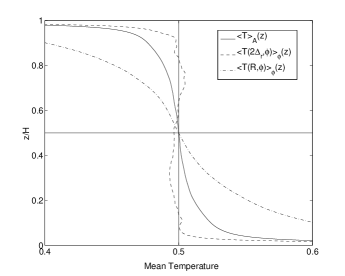
Figure 1 shows the vertical mean temperature profiles taken in three different ways in the turbulent flow for a Rayleigh number . The standard mean temperature profile is compared with two vertical mean temperature profiles which are conducted at fixed radial positions and averaged azimuthally, . It can be seen that the slopes of the temperature vary significantly. While the profile has almost zero slope at , a destabilizing slope, , is observed close to the sidewall. Close to the centre line, the situation is reversed, we observe a stabilizing slope, . Our finding agrees with a recent experiment by Brown & Ahlers (2007) and confirms that the assumption of the temperature drop across the thermal boundary layer is a simplification. The presence of a non-vanishing local mean temperature gradient can have an impact on the statistics of the small-scale temperature fluctuations, similar to the passive scalar case. This point will be discussed further in section 3.
The thermal boundary layer is resolved with at least 14 lateral grid planes for all runs.
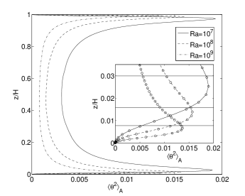
This is indicated in Fig. 2 where we plot the vertical mean square profiles of the temperature fluctuations and highlight the (non-equidistant) vertical grid spacing by the symbols in the inset. The horizontal lines correspond to the thermal boundary layer thickness estimated by , which is always close to the position of the maximum of . All runs were performed for at least 80 large-scale eddy turnover times in order to gather sufficient statistics. We also verified that the vertical Nusselt number profile given by
| (10) |
is a constant with a standard deviation of about . The mean value of the Nusselt number profile,
| (11) |
follows the scaling law , with and .
3 Temperature and its derivative statistics
3.1 Total temperature and its fluctuations
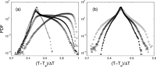
Figure 3 shows the probability density functions (PDF) of the dimensionless temperature at different heights from the bottom plate and as a function of the Rayleigh number, respectively. The findings are in agreement with Siggia (1994) and Kerr (1996). As expected, the PDFs in Fig. 3a become increasingly symmetric toward the centre of the convection cell. This height-dependent asymmetry can be measured alternatively by the skewness of the temperature fluctuations, , which is given by
| (12) |
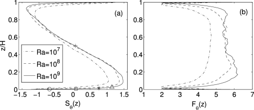
The graphs are shown in Fig. 4a. A small skewness around implies that rising and falling plumes are observed at the edge of the bottom and top thermal boundary layers. Simultaneously, the colder and hotter pockets of temperature are generated in the vicinity of the thermal plumes which detach from the thermal boundary layer. This is a consequence of the incompressibility of the fluid as investigated more detailed in the Lagrangian frame of reference by Schumacher (2008). Up to a height of , the skewness increases monotonically before it declines to zero at the cell centre plane. The plots show that the maximum value of skewness increases with increasing Rayleigh number. A large positive value of the skewness close to the bottom plate means that rising plumes with are dominant in this region of the convection cell. This is exactly the region in which a cusp is forming at in the PDF (see Fig. 3a).
The distribution of the temperature in the centre plane () of the cell as a function of the Rayleigh number is shown in Fig. 3b. The profiles are clearly non-Gaussian for all three Rayleigh numbers. The support of the PDF becomes narrower with increasing . The PDF for the fluctuations has the same shape in the centre plane. We found that the PDFs of for the two larger Rayleigh numbers collapse when the temperature fluctuation is normalized by the corresponding root-mean-square value, , at . The PDF for has slightly smaller tails. The magnitude of the deviations from Gaussianity can be measured by the flatness which is given by
| (13) |
Figure 4b shows the vertical profiles of the flatness for the three Rayleigh numbers. The non-Gaussianity, i.e., a flatness larger than 3, is present for all three . This is in agreement with other studies such as by Heslot et al. (1987), Castaing et al. (1989) or Ching (1991). It can also be observed that the flatness value levels off in the cell centre for the two larger Rayleigh numbers. This could indicate that the transition to the so-called hard turbulence regime of convection has been completed. Dimotakis (2005) discussed a mixing transition for passive scalars at . Above this threshold, a weaker dependence was predicted. A similar behaviour could be the reason for our observation. All flatness profiles have a minimum right above the thermal boundary layer. The slight asymmetry of the profile at is due to limitations in the statistical analysis. Even a longer time advancement and 140 statistically independent snapshots were not sufficient to obtain a symmetric profile since this analysis of the higher-order moments is done plane by plane.
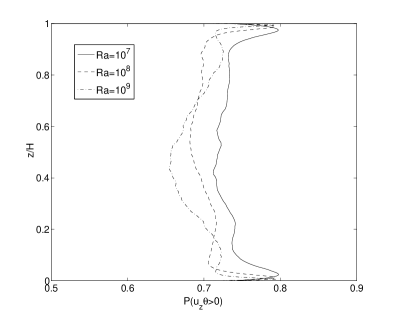
As already seen, the non-Gaussian PDF of the total temperature and the temperature fluctuations in the cell centre is a robust feature in thermal convection. It has been reported in experiments starting with Heslot et al. (1987) and Castaing et al. (1989). An almost exponential shape was emphasized by Yakhot (1989) on the basis of a hierarchy of moment equations for the temperature fluctuations. These ideas have been extended by Ching (1993) later. Yakhot suggested that this form prevails even for moderate Rayleigh numbers (which implies moderate Reynolds numbers), whenever regions with are dominant. A correlation between the vertical velocity and temperature fluctuation is nothing else but a fingerprint of a local blob of heat transferred through the cell. Inspection of our data yields indeed that larger regions with are present everywhere in the cell, even in the centre where coherent plumes are absent. This is shown in Fig. 5 where we plot the vertical dependence of the probability for three different Rayleigh numbers. It can be clearly seen that the probability decreases with increasing Rayleigh number, but remains significantly larger than 0.5 for all three cases. The plot is another manifestation of the net transfer of heat through the cell.
Interestingly, the passive scalar turns out to be more sensitive to a particular driving and the Reynolds number of the advecting flow. When a mean scalar gradient is absent, the statistics is close to Gaussian or sub-Gaussian such as in Mydlarski & Warhaft (1998) or Watanabe & Gotoh (2004). In case of a non-vanishing mean scalar gradient, Pumir et al. (1991) suggested an exponentially distributed passive scalar as a generic feature, based on a simple one-dimensional random advection model. This was confirmed experimentally for sufficiently high Reynolds numbers (Gollub et al. 1991; Jayesh & Warhaft 1991; Jayesh & Warhaft 1992). However, sub-Gaussian distributions of have also been found for this case by Overholt & Pope (1996), Ferchichi & Tavoularis (2002) and Schumacher & Sreenivasan (2005). Experiments by Gylfasson & Warhaft (2004) detected that the statistics depends on the particular driving of the turbulent flow. While an active grid caused sub-Gaussian fluctuations, a fine static grid caused super-Gaussian passive scalar distributions. Furthermore the deviations from Gaussian distributions decreased with increasing downstream distance in their experiments. The two findings imply that the ratio of the integral scales to the system scale is important. This is a point which has to be addressed more detailed.
3.2 Vertical derivative of temperature fluctuations
An important question in turbulent convection is if the fluctuations of the temperature field in the bulk can be considered as being locally isotropic. In order to shed light on this point we adopt an approach that has been used successfully for passive scalars with a mean scalar gradient (Warhaft 2000). As we have seen in section 2, the local mean temperature gradient can deviate from zero while the overall profile sums up to a mean temperature gradient which is almost zero (see Fig. 1). Following Brown & Ahlers (2007), we define a ratio that relates a difference of azimuthally averaged mean temperatures at fixed radial distance to the total temperature drop. It is given by
| (14) |
Close to the side wall, we get for , for and for . This large slope is mainly due to the rising and falling plumes. At the centre line, it follows for , for and for . Although decreasing with increasing Rayleigh number for both cases, their magnitude is not negligible. We observe that local mean temperature gradients are present. This supports the idea to conduct an analysis similar to passive scalar turbulence.
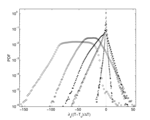
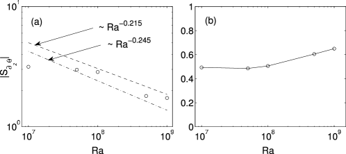
The statistics of the vertical derivative of the temperature, , is shown in Fig. 6. The PDFs are analysed at the same heights as those for the temperature in Fig. 3a. A sharp decrease of the PDF at is present in the vicinity of , simply because positive vertical derivatives are very unprobable close to the bottom plate. With increasing distance from the plate, the support of the PDF decreases. A negative skewness of all distributions can be observed which implies preferential derivatives along the mean negative temperature gradient. Recall also that a turbulent field is thought to be perfectly locally isotropic when all odd-order derivative moments are exactly zero. Therefore, the derivative skewness with respect to the temperature fluctuations , defined as
| (15) |
is presented here. It measures deviations from the local isotropy at the smaller scales of convective turbulence. Figure 7 shows that such deviations are indeed present in different regions of the cylindrical domain. With increasing Rayleigh number and thus increasing Reynolds number, the derivative skewness decreases in magnitude in the centre region (see Fig. 7a). Following the original idea on the return to local isotropy in a simple shear flow (Lumley 1967) and its adaption to the passive scalar case (Warhaft 2000), a return would require a rather rapid decay law of the skewness with respect to the Taylor microscale Reynolds number , i.e. . This was not found in passive scalar case for Schmidt numbers around unity (Warhaft 2000). Given the scaling dependence of the Reynolds number with respect to the Rayleigh number, which will be discussed more detailed in section 4.1, and the relation , a return to local isotropy in convection would require a decay law which is given by
| (16) |
for a fixed . Here is the scaling exponent for relation, which was found to vary between and 0.49 in experiments (see section 4.1). Figure 7a indicates that our data follow such a decay law for the larger Rayleigh numbers. This is in line with the observation that the local mean gradients in the bulk decrease in magnitude with increasing . The mean temperature gradient still causes ramps and cliffs of the temperature and thus a non-vanishing derivative skewness, but its impact seems to be weaker compared to a passive scalar which lacks a return to isotropy. A larger range of Rayleigh numbers and the analysis of the hyperskewness would allow to draw a firm conclusion.
The opposite trend with respect to the Rayleigh number can be observed in the thermal boundary layer where the skewness is increasing in magnitude with Rayleigh number (see Fig. 7b). Figure 6 shows that particularly the PDFs in the boundary layer are strongly skewed to negative derivatives. This observation is due to the fact that the heat transfer is mostly contributed by the second term of (10) there and that the fluctuations about the mean are consequently dominated by the conductive contributions . We will come back to this point in the next section when discussing the height dependence of the thermal dissipation.
4 Thermal dissipation rate
4.1 Vertical profiles and Rayleigh number scaling
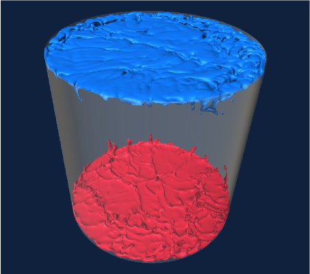
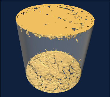
Figure 8 represents the isosurface plots of a snapshot of (top) and of (bottom) at . We recognize the ridges in the temperature isosurface which correspond to the plumes that are detached from the bottom and top boundary layers. Associated with the rising and descending plumes are larger amplitudes of the thermal dissipation field which can be observed in the bottom panel, similar to findings by Kerr (1996) or Shishkina & Wagner (2007). The pattern of ridges (or stems) in the top panel is recaptured almost one-to-one in the bottom panel. The isosurface plot in the bottom panel indicates also that the local maxima of the thermal dissipation field are dominantly found close to both plates and not in the cell centre.
In order to quantify this vertical dependence more precisely, we decompose the thermal dissipation rate field into contributions which result from the mean temperature profile and the temperature fluctuations. With (3), it follows
| (17) | |||||
| (18) |
The mixed term vanishes after averaging over planes at fixed height and thus
| (19) |
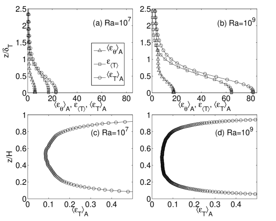
Figure 9 plots the vertical profiles of both contributions to the total thermal dissipation rate for Rayleigh numbers (left column) and (right column). All values of the thermal dissipation fields are given in units of the corresponding ensemble mean, (see also (2)). The contribution of the mean temperature profile, , is dominant in the thermal boundary layer and decreases rapidly to almost zero toward the cell centre (see panels (a) and (b)). This mean profile contribution increases with increasing Rayleigh number since the scale across which the significant temperature variation appears, , becomes smaller. Conversely, the thermal dissipation rate due to the temperature fluctuations is dominant in the bulk and exceeds the mean profile contribution by more than 3 orders of magnitude there (not shown). As displayed in panels (c) and (d) of Fig. 9 for both Rayleigh numbers, the total dissipation remains significantly below in the cell centre.
From (2) and the scaling relation , the Rayleigh-number dependence of the ensemble average yields
| (20) |
which gives an exponent in our simulations. This global scaling can be refined for different subvolumes of the cylindrical domain. Well in the centre, we define the bulk dissipation as
| (21) |
The thermal dissipation in the boundary layer is given by
| (22) |
In line with the definitions of averages in section 2, we combine again an average over many realizations of the turbulent fields and a volume average which is taken now over the subvolumes and as defined in (21) and (22), respectively. Following Grossmann & Lohse (2000) (see their eq. (2.15)), one can estimate the thermal dissipation in the thermal boundary layer by assuming that it is due to the mean temperature drop across only and that . This leads to
| (23) |
The factor stands for the fraction of the total volume which is occupied by the boundary layer. The last step in (23) holds if is a constant. For Rayleigh numbers between and , our DNS give a scaling with respect to Rayleigh number of
| (24) |
This exponent is significantly smaller than the predictions by the scaling theories, or 1/3. We conclude that (23) is not capturing the significant contribution from which can also be seen in Fig. 9. In addition, we find that displays almost the same scaling with Rayleigh number as in our direct numerical simulations.
In the bulk of the cylindrical cell, the thermal dissipation rate is due to temperature fluctuations only and can be estimated by (see eq. (2.12) in Grossmann & Lohse (2000))
| (25) |
Further explanation requires the knowledge of . Corresponding to experiments, an anomalous scaling dependence of the Reynolds number on the Rayleigh number is found, i.e. deviations from a scaling exponent of (Grossmann & Lohse 2002; Brown et al. 2007a). Furthermore, the definition of the Reynolds number, especially the choice of the characteristic velocity, leads to additional variations in the exponents. In summary, the range of exponents is found to be between and 0.49. It follows thus from (25) that
| (26) |
for a fixed Prandtl number, as in the present study, with an exponent . However, our numerical simulations lead to
| (27) |
which comes close to the experimental findings by He et al. (2007) and exhibits the reported trend of Verzicco & Camussi (2003). It does not vary significantly if the bulk volume fraction is increased in the analysis. For example, an exponent of in (27) was obtained in the region . The Rayleigh number range, for which this least square fit was taken, is between and . We conclude that the scaling exponent, which is by the way rather robust with respect to changes of the volume fraction, has the opposite sign in contrast to the scaling based on the estimate by Grossmann & Lohse (2000). The reason for this discrepancy could be that the dimensionally correct ansatz may not be appropriate for the thermal dissipation rate. Similar to fluid turbulence, the Rayleigh numbers (and therefore the Reynolds numbers) are still too small to reach the regime where the thermal dissipation rate given in units of is a constant. This is known as the dissipation anomaly (Donzis, Sreenivasan & Yeung, 2005). Both and still decrease with increasing for our data record ( defined as described in the caption of table 1).
4.2 Stretched exponential behaviour in the tails
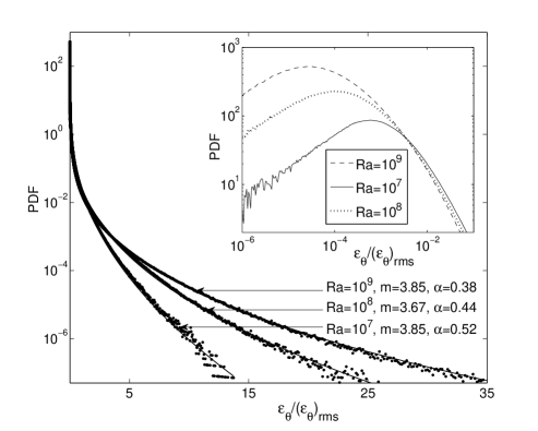
The mismatch of the Rayleigh number scaling with the predictions by Grossmann & Lohse (2000) suggests that strong fluctuations of the thermal dissipation were not taken into account in the scaling. We discuss therefore the statistics of in this section. Figure 10 shows the PDF of the dissipation rate of temperature fluctuations in the bulk. The analysis is conducted in planes between . In correspondence with the passive scalar case (Overholt & Pope, 1996; Schumacher & Sreenivasan, 2005), we fit a stretched exponential to the fraction of the PDF which extends from the most probable amplitude (see the inset of Fig. 10) to the end of the tail. We define and , with is the abscissa of the most probable (mp) value. Data are fitted to
| (28) |
Similar to the passive scalar case, we do observe fatter tails with increasing Rayleigh number (and therefore with increasing Reynolds number). This is in line with an increasing degree of small-scale intermittency of the thermal dissipation rate field. Overholt & Pope (1996) and Schumacher & Sreenivasan (2005) have conducted a similar analysis for the passive scalar dissipation rate in a homogeneous isotropic turbulent flow. There, a minimal exponent can be derived analytically in the limit of a very large Peclét number. The scalar is then advected in a flow which is white in time (Chertkov et al. 1998, Gamba & Kolokolov 1999). The advection of a passive scalar in a Navier-Stokes flow always resulted in tails that were sparser, i.e. (Yeung et al. 2005). Our present analysis indicates that this threshold is also approached for the hard-turbulence regime of convection.
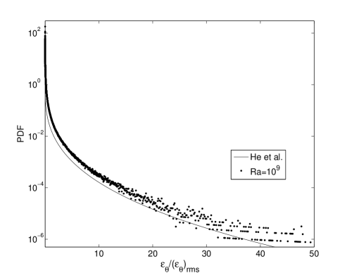
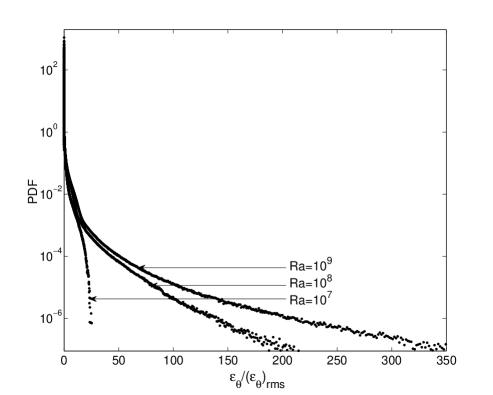
Figure 11 replots our data in the center plane for in units of the rms value of thermal dissipation in order to compare them with the measurements by He et al. (2007). A slightly sparser tail in the experiments is observed. On the one hand, the reason for this difference might be due to the improved resolution of the temperature gradient in our simulations, which was not possible in the experiment, as mentioned before. On the other hand, the Prandtl number () was almost an order of magnitude larger in the experiment. An increasing Prandtl number reduces the thermal boundary layer thickness and can cause less plume mixing in the bulk. Less pronounced plumes will cause smaller amplitudes of the thermal dissipation. Such a trend with the Prandtl number would differ from passive scalar turbulence, where the tails of the PDF of become fatter with increasing Prandtl (or Schmidt) number at a given Reynolds number of the advecting flow (Schumacher & Sreenivasan, 2005). There a less diffusive scalar field generates sharper gradients. It remains open which of those two effects is more dominant. Further simulations are required to study the dependence of the temperature gradient statistics on the Prandtl number in thermal convection.
When repeating the analysis for the part of the volume () that has been excluded before, distributions as shown in Fig. 12 result. It is observed that the amplitudes of the dissipation increase by an order of magnitude for the largest compared to Fig. 10. The fatter tails for the boundary layer data are in line with the analysis of the vertical plane averaged profiles (see Fig. 9). The fluctuations of the thermal dissipation rate increase with increasing .
4.3 Deviations from log-normality
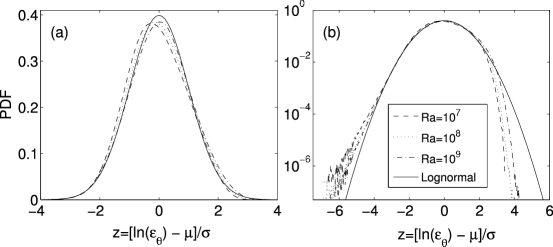
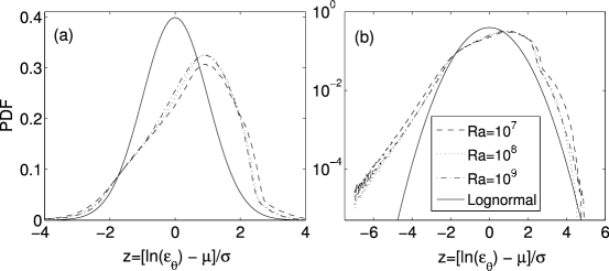
The intermittent nature of the thermal dissipation field leads to deviations from log-normality, as can be seen in Fig. 13 where the same data set has been studied as in Fig. 10. In order to highlight the differences in PDFs, we represent the data in linear-linear and linear-logarithmic axes respectively. It can be seen that neither the core nor both tails of the PDF fit perfectly. This is similar to the passive scalar mixing. Small-amplitude tails are fatter than the log-normal curve while large-amplitude tails remain sparser (Ferchichi & Tavoularis 2002, Schumacher & Sreenivasan 2005). The trend of the data with Rayleigh numbers between and suggests a very slow convergence towards the log-normality. The repetition of the analysis in the vicinity of the thermal boundary layers, i.e. for the same data set as in Fig. 12, reveals even stronger deviations (see Fig. 14). For the large-amplitude tail, a bump is observed. A similar feature has been reported by Kaczorowski & Wagner (2007). Our analysis suggests that this particular feature is due to the boundary layer dynamics. The bump in the distribution remains also when the PDF is analysed for the whole cell and not for a particular subvolume.
4.4 Conditional mean thermal dissipation
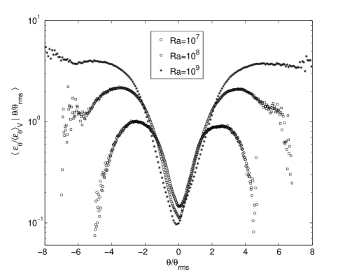
Deviations from the Gaussian distributions of the temperature fluctuation are also manifested in the conditional mean thermal dissipation. It is known that a conditional mean scalar dissipation is constant for a Gaussian scalar field, i.e. independent with respect to the scalar amplitude (see e.g. Overholt & Pope 1996). The mean is defined as
| (29) |
where is the joint PDF of the thermal dissipation rate and the temperature fluctuation. Figure 15 displays clearly the V-shape for the conditional mean for temperature fluctuation values around . This is consistent with the deviations from Gaussianity, which were detected for the distributions of the temperature field. At larger magnitudes of , the graphs reach a maximum before decreasing to zero since the support of the joint PDF and the temperature PDF is bounded. The V-shape is more pronounced with increasing Rayleigh number which is due to the higher thermal dissipation amplitudes observable in the flow (see Fig. 10). Our results agree with the findings of Jayesh & Warhaft (1992).
5 Conclusions
We have presented a detailed numerical study of the statistics of the temperature fluctuations and their gradients in turbulent convection. The resolution constraints limited the study to moderate Rayleigh numbers between and . We compared the fine-scale structure of the active temperature field to that of the passive scalar field, far away from the boundaries. In contrast to the passive scalar case, the temperature statistics is always non-Gaussian with a probability density function close to exponential in the bulk. Non-Gaussianity holds in all regions of the convection cell and for all mentioned Rayleigh numbers. Deviations in temperature fluctuations from the Gaussian distribution have also been confirmed by the V-shaped conditional mean dissipation. For the passive scalar fluctuations, the statistics depends on the mechanism that sustains the fluctuations and on the particular ratios of outer turbulence length scales. Super-Gaussian, Gausisan or weakly sub-Gaussian distributions have been observed there in the past. While the statistics of the temperature can differ from the passive scalar, the statistics of the spatial derivatives and dissipation rates behave qualitatively similarly.
The probability density function of the thermal dissipation rate in the bulk is fitted well with a stretched exponential. The tails extend to larger amplitudes with increasing Rayleigh number. This is a clear fingerprint of a stronger small-scale intermittency. Thermal dissipation field is always more intermittent in the boundary layer than the bulk of the convection cell. This is indicated by the extended tail of the PDF. All distributions showed clear deviations from the log-normality in the whole range of dissipation values.
Motivated by similar studies in passive scalar turbulence and by our detection of locally varying mean temperature profiles, the deviations from locally isotropic temperature fluctuations are quantified by the third order vertical derivative moments as a function of the Rayleigh number. Interestingly, we found that the deviations from the local isotropy grow with increasing in the boundary layer. In the bulk, the derivative skewness is found to decrease. Our data exhibit return to isotropy trend (Lumley 1967) when translating the original Reynolds number dependence of the skewness into a Rayleigh number dependence for the convection case. This is in contrast to the passive scalar case which does not show such trend (Warhaft 2000). The observed return might be due to the small amplitudes that the local mean temperature gradients possess. The vertical profiles of the plane averaged thermal dissipation show furthermore that an increasing fraction is concentrated in an ever thinner boundary layer with growing . Finally, we demonstrate that the contribution of the temperature fluctuations to the total thermal dissipation in the thermal boundary layer is significant and cannot be neglected. This aspect is not included in the scaling of the thermal dissipation rate with respect to the Rayleigh number and can explain why the present trends of the total thermal dissipation with respect to the Rayleigh number differ in comparison to the scaling theory by Grossmann & Lohse (2000).
Two aspects will be addressed in our future work on this subject. Firstly, an extension to larger aspect ratios and higher Rayleigh numbers is desirable. It is known from experiments, such as by du Puits et al. (2007a), that the large-scale motion is sensitive to the aspect ratio. A rearrangement of the large-scale flow patterns will consequently affect the statistics of various quantities. Secondly, the direct link between the observed statistics and the local structures in the boundary layer and its vicinity is necessary. First steps have been done already in Shishkina & Wagner (2007) and Zhou et al. (2007). Our investigations on both aspects have started recently and will be discussed elsewhere.
Acknowledgements.
We would like to thank first Roberto Verzicco for providing us his simulation code and his help at the beginning of our studies. We acknowledge discussions with Norbert Peters, Katepalli R. Sreenivasan and André Thess. We also thank for supercomputing ressources on the IBM p690 cluster JUMP of the Jülich Supercomputing Centre (Germany) under grant HMR09. The work is supported by the Deutsche Forschungsgemeinschaft (DFG) under grant SCHU1410/2 and by the Heisenberg Program of the DFG. We also wish to thank all three referees for their constructive comments and suggestions.References
- Belmonte (1994) Belmonte A., Tilgner, A. & Libchaber, A. 1994 Temperature and velocity boundary layers in turbulent convection. Phys. Rev. E 50, 269-279.
- Belmonte (1996) Belmonte A. & Libchaber, A. 1996 Thermal signature of plumes in turbulent convection: The skewness of the derivative. Phys. Rev. E 53, 4893-4898.
- Brown (2007) Brown, E. & Ahlers, G. 2007 Temperature gradients, and search for non-Boussinesq effects, in the interior of turbulent Rayleigh-Bénard convection. Europhys. Lett. 80, 14001 (6 pages).
- Brown (2007a) Brown, E., Funfschilling, D. & Ahlers, G. 2007a Anomalous Reynolds-number scaling in turbulent Rayleigh-Bénard convection. J. Stat. Mech. P10005.
- Castaing (1989) Castaing, B., Gunaratne, G., Heslot, F., Kadanoff, L., Libchaber, A., Thomae, S., Wu, X.-Z., Zaleski, S. & Zanetti, G. 1989 Scaling of hard thermal turbulence in Rayleigh-Bénard convection. J. Fluid Mech. 204, 1-30.
- Castaing (1990) Castaing, B., Gagne, Y. & Hopfinger, E. J. 1990 Velocity probability density functions of high Reynolds number turbulence. Physica D 46, 177-200.
- Chertkov (1998) Chertkov, M., Falkovich, G. & Kolokolov, I. 1998 Intermittent dissipation of a passive scalar in turbulence. Phys. Rev. Lett. 80, 2121-2124.
- Chevillard (2006) Chevillard, L., Castaing, B., Lévêque & Arneodo, A. 2006 Unified multifractal description of velocity increments statistics in turbulence: Intermittency and skewness. Physica D 218, 77-82.
- Ching (1991) Ching, E. S. C. 1991 Probabilities for temperature differences in Rayleigh-Bénard convection. Phys. Rev. A 44, 3622-3628.
- Ching (1993) Ching, E. S. C. 1993 Probability densities of turbulent temperature fluctuations. Phys. Rev. Lett. 70, 283-286.
- Dimotakis (2005) Dimotakis, P. E. 2005 Turbulent mixing. Annu. Rev. Fluid Mech. 37 329-356.
- Donzis (2005) Donzis, D. A., Sreenivasan, K. R. & Yeung, P. K. 2005 Scalar dissipation rate and dissipative anomaly in isotropic turbulence. J. Fluid Mech. 532, 199-216.
- du Puits (2007) du Puits, R., Resagk, C., Tilgner, A., Busse, F.-H. & Thess, A. 2007 Structure of thermal boundary layers in turbulent Rayleigh-Bénard convection. J. Fluid Mech. 572, 231-254.
- du Puits (2007a) du Puits, R., Resagk, C. & Thess, A. 2007a Breakdown of wind in turbulent thermal convection. Phys. Rev. E 75, 016302 (4 pages).
- Ferchichi (2002) Ferchichi, M. & Tavoularis, S. 2002 Scalar probability density function and fine structure in uniformly sheared turbulence. J. Fluid Mech. 461, 155-182.
- Funfschilling (2005) Funfschilling, D., Brown, E., Nikolaenko, A. & Ahlers, G. 2005 Heat transport by turbulent Rayleigh-Bénard convection in cylindrical samples with aspect ratio one and larger. J. Fluid Mech. 536, 145-154.
- Gamba (1999) Gamba A. & Kolokolov, I. 1999 Dissipation statistics of a passive scalar in a multi-dimensional smooth flow. J. Stat. Phys. 94, 759-777.
- Gollub (1991) Gollub, J. P., Clarke, J., Gharib, M., Lane, B. & Mesquita, O. N. 1991 Fluctuations and transport in a stirred fluid with a mean gradient. Phys. Rev. Lett. 67, 3507-3510.
- Groetzbach (1983) Grötzbach, G. 1983 Spatial resolution requirements for direct numerical simulation of the Rayleigh-Bénard convection. J. Comput. Phys. 49, 241-269.
- Grossmann (2000) Grossmann, S. & Lohse, D. 2000 Scaling in thermal convection: a unifying theory. J. Fluid Mech. 407, 27-56.
- Grossmann (2002) Grossmann, S. & Lohse, D. 2002 Prandtl and Rayleigh number dependence of the Reynolds number in turbulent thermal convection. Phys. Rev. E 66, 016305 (6 pages).
- Gylfason (2004) Gylfason, A. & Warhaft, Z. 2004 On higher order passive scalar structure functions in grid turbulence. Phys. Fluids 16, 4012-4019.
- Hartlep (2005) Hartlep, T., Tilgner, A. & Busse, F. H. 2005 Transition to turbulent convection in a fluid layer heated from below at moderate aspect ratio. J. Fluid Mech. 544, 309-322.
- He (2007) He, X., Tong, P. & Xia, K.-Q. 2007 Measured thermal dissipation field in turbulent Rayleigh-Bénard convection. Phys. Rev. Lett. 98, 144501 (4 pages).
- Heslot (1987) Heslot, F., Castaing, B. & Libchaber, A. 1987 Transitions to turbulence in helium gas. Phys. Rev. A 36, 5870-5873.
- Jayesh (1991) Jayesh & Warhaft, Z. 1991 Probability distribution of a passive scalar in grid-generated turbulence. Phys. Rev. Lett. 67, 3503-3506.
- Jayesh (1992) Jayesh & Warhaft, Z. 1992 Probability distribution, conditional dissipation and transport of passive temperature fluctuations in grid-generated turbulence. Phys. Fluids A 4, 2292-2307.
- Kadanoff (2001) Kadanoff, L. P. 2001 Turbulent heat flow: Structures and scaling. Phys. Today 54, 34-99.
- Kaczorowski (2007) Kaczorowski, M. & Wagner C. 2007 Direct numerical simulation of turbulent convection in a rectangular Rayleigh-Bénard cell. Proceedings of Fifth International Symposium on Turbulence and Shear Flow Phenomena, Garching, 2007, Vol.2, 499-504.
- Kerr (1996) Kerr, R. M. 1996 Rayleigh number scaling in numerical convection. J. Fluid Mech. 310, 139-179.
- Kushnir (2006) Kushnir, D., Schumacher, J. & Brandt, A. 2006 Geometry of intensive scalar dissipation events in turbulence. Phys. Rev. Lett. 97, 124502.
- Lumley (1967) Lumley, J. L. 1967 Similarity and the turbulent energy spectrum. Phys. Fluids 10, 855-858.
- Mydlarski (1998) Mydlarski, L. & Warhaft, Z. 1998 Passive scalar statistics in high-Péclet-number grid turbulence. J. Fluid Mech. 358, 135-175.
- Niemela (2000) Niemela, J. J., Skrbek, L., Sreenivasan, K. R. & Donelly, R. J. 2000 Turbulent convection at very high Rayleigh numbers. Nature 404, 837-840.
- Niemela (2003) Niemela, J. J. & Sreenivasan, K. R. 2003 Turbulent confined convection. J. Fluid Mech. 481, 355-384.
- Overholt (1996) Overholt, M. R. & Pope, S. B. 1996 Direct numerical simulation of a passive scalar with imposed mean gradient in isotropic turbulence. Phys. Fluids 8, 3128-3148.
- Pumir (1996) Pumir, A. 1996 Turbulence in homogeneous shear flows. Phys. Fluids 8, 3112-3127.
- Pumir (1991) Pumir, A., Shraiman, B. & Siggia, E. D. 1991 Exponential tails and random advection. Phys. Rev. Lett. 23, 2984-2987.
- Schumacher (2003) Schumacher, J. & Sreenivasan, K. R. 2003 Geometric features of the mixing of passive scalars at high Schmidt numbers. Phys. Rev. Lett. 91, 174501 (4 pages).
- Schumacher (2005) Schumacher, J., Sreenivasan, K. R. & Yeung, P. K. 2005 Very fine structures in scalar mixing. J. Fluid Mech. 531, 113-122.
- Schumacher (2005) Schumacher, J.& Sreenivasan, K. R. 2005 Statistics and geometry of passive scalars in turbulence. Phys. Fluids 17, 125107 (9 pages).
- Schumacher (2008) Schumacher, J. 2008 Lagrangian dispersion and heat transport in convective turbulence. Phys. Rev. Lett. 100, 134502 (4 pages).
- Shishkina (2006) Shishkina, O. & Wagner C. 2006 Analysis of thermal dissipation rates in turbulent Rayleigh-Bénard convection. J. Fluid Mech. 546, 51-60.
- Shishkina (2007) Shishkina, O. & Wagner C. 2007 Local heat flux in turbulent Rayleigh-Bénard convection. Phys. Fluids 19, 085107 (13 pages).
- Shraiman (2000) Shraiman, B. I. & Siggia E. D. 2000 Scalar turbulence. Nature 405, 639-646.
- Siggia (1994) Siggia E. D. 1994 High Rayleigh number convection. Annu. Rev. Fluid Mech. 26 137-68.
- Verzicco (2003) Verzicco, R. & Camussi, R. 2003 Numerical experiments on strongly turbulent thermal convection in a slender cylindrical cell. J. Fluid Mech. 477, 19-49.
- Verzicco (1996) Verzicco, R. & Orlandi, P. 1996 A finite-difference scheme for three-dimensional incompressible flows in cylindrical coordinates. J. Comp. Phys. 123, 402-414.
- Warhaft (2000) Warhaft, Z. 2000 Passive scalars in turbulent flows. Annu. Rev. Fluid Mech. 32, 203-240.
- Warhaft (2002) Warhaft, Z. 2002 Turbulence in nature and laboratory. Proc. Nat. Acad. Sci. 99, 2481-2486.
- Watanabe (2004) Watanabe, T. & Gotoh, T. 2004 Statistics of a passive scalar in homogeneous turbulence. New J. Phys. 6, 40 (36 pages).
- Xi (2004) Xi, H.-D., Lam, S. & Xia, K.-Q. 2004 From laminar plumes to organized flows: the onset of large-scale circulation in turbulent thermal convection. J. Fluid Mech. 503, 47-56.
- Yakhot (1989) Yakhot, V. 1989 Probability distributions in high-Rayleigh-number Bénard convection. Phys. Rev. Lett. 63 1965-1967.
- Yeung (2005) Yeung, P. K., Donzis, D. A. & Sreenivasan, K. R. 2005 High-Reynolds-number simulation of turbulent mixing. Phys. Fluids 17 081703 (4 pages).
- Zhou (2002) Zhou S.-Q. & Xia, K.-Q. 2002 Plume statistics in thermal turbulence: Mixing of an active scalar. Phys. Rev. Lett. 89, 184502 (4 pages).
- Zhou (2007) Zhou Q., Sun, C. & Xia, K.-Q. 2007 Morphological evolution of thermal plumes in turbulent Rayleigh-Bénard convection. Phys. Rev. Lett. 98, 074501 (4 pages).