Star formation histories from multiband photometry: A new approach

Abstract

A new method of determining galaxy star-formation histories (SFHs) is presented. Using the method, the feasibility of recovering SFHs with multi-band photometry is investigated. The method divides a galaxy’s history into discrete time intervals and reconstructs the average rate of star formation in each interval. This directly gives the total stellar mass. A simple linear inversion solves the problem of finding the most likely discretised SFH for a given set of galaxy parameters. It is shown how formulating the method within a Bayesian framework lets the data simultaneously select the optimal regularisation strength and the most appropriate number of discrete time intervals for the reconstructed SFH. The method is demonstrated by applying it to mono-metallic synthetic photometric catalogues created with different input SFHs, assessing how the accuracy of the recovered SFHs and stellar masses depend on the photometric passband set, signal-to-noise and redshift. The results show that reconstruction of SFHs using multi-band photometry is possible, being able to distinguish an early burst of star formation from a late one, provided an appropriate passband set is used. Although the resolution of the recovered SFHs is on average inferior compared to what can be achieved with spectroscopic data, the multi-band approach can process a significantly larger number of galaxies per unit exposure time.

1 Introduction

A significant step towards understanding how galaxies form and evolve can be made by measuring the variation in their star formation rate (SFR) with age. Imprinted in every galaxy’s integrated light is a record of its entire life from birth, through passive evolution, possible merging and recycling of material, up to the epoch at which it is observed. Star formation histories (SFHs) therefore play a crucial role in the quest for a complete and accurate model of the formation of stellar mass in the Universe and how distant systems relate to those locally.

Characterising galaxy SFHs has been a subject of much interest for several decades, with studies attempting to achieve this aim through a variety of different means. Approaches can be broadly divided into those using multi-band photometry and those using spectra. Recently the practice has seen a significant revival thanks to improvements in stellar synthesis modelling and the advent of large datasets such as the Sloan Digital Sky Survey (SDSS; Stoughton et al., 2002). Many new spectroscopic techniques have been developed (e.g., Heavens, Jimenez & Lahav, 2000; Vergeley, Lançon & Mouhcine, 2002; Cid Fernandes et al., 2004, 2005; Nolan et al., 2006; Ocvirk et al., 2006; Chilingarian et al., 2007; Tojeiro et al., 2007) and in their various forms, these have seen application to several sets of real data (e.g., Reichardt, Jimenez & Heavens, 2001; Panter, Heavens & Jimenez, 2003; Heavens et al., 2004; Panter, Heavens & Jimenez, 2004; Sheth et al., 2006; Cid Fernandes et al., 2007; Nolan et al., 2007; Panter et al., 2007; Koleva et al., 2008). Similarly, there have been numerous recent studies conducted using multi-band photometry (e.g., Borch et al., 2006; Schawinski et al., 2007; Salim et al., 2007; Noeske et al., 2007; Kaviraj et al., 2007) including Kauffmann et al. (2003) who combined multi-band photometry with measurements of the H$\delta$ absorption line and 4000Åbreak strength.

In a similar vein to spectroscopic versus photometric redshift estimation, SFHs determined from spectra tend to have greater precision per galaxy, whereas those derived from multi-band photometry allow many more objects to be studied in the same amount of observing time but with a compromise in SFH resolution. The method adopted by existing multi-band studies is to assume a parametric model for the SFH. The parameters are adjusted to find the set of model fluxes, computed from a spectral library of choice, that best matches the set of observed fluxes. This not only forces the SFH to adhere to a potentially unrepresentative prescribed form, it also necessitates a fully non-linear minimisation over all parameters.

In contrast, the majority of the recent spectroscopic methods divide up a galaxy’s history into several independent time intervals and reconstruct the average SFR in each interval to give a discretised SFH. The advantage this brings, as shown in Section 2.2, is that finding the best-fit SFR in every interval for a fixed set of galaxy parameters (such as redshift, extinction and metallicity) is a linear problem. The inefficient non-linear SFH minimisation with its risk of becoming trapped in local minima is therefore replaced with a simple matrix inversion guaranteeing that the global minimum for the fixed set of galaxy parameters is found.

The prescribed SFH models used by the multi-band methods are mainly driven by the small number of passbands used in many multi-band campaigns. With only a small number of passbands, the ability to constrain a galaxy’s SFH is limited and a model SFH with only one or two parameters must be used. However, modern surveys are being carried out in many more passbands and over larger wavelength ranges than ever before (for example, the COMBO-17 survey of Wolf et al., 2001). Given these recent improvements, the possibility of recovering discretised SFHs from multi-band photometry alone is now worthy of investigation.

The purpose of this paper is twofold. Firstly, a new SFH reconstruction method that recovers discretised SFHs is presented. It is shown how the Bayesian evidence can be used to simultaneously establish the most appropriate number of discrete SFH time intervals and the optimal strength with which the solution should be regularised. The formalism is completely general and can be applied to spectra just as easily as multi-band photometry as well as a combination of both. The Bayesian evidence gives a more natural and simplified alternative to existing procedures for determining the optimal number of SFH intervals and for determining the correct level of regularisation.

Secondly, this paper presents results of an investigation into the feasibility of using the new method with multi-band photometry alone. By applying the method to synthetic galaxy catalogues created with different input SFHs and filtersets, the accuracy of the recovered discretised SFHs is demonstrated. This study focuses in particular on the dependence of the reconstruction on galaxy redshift, photometric signal-to-noise (S/N), the wavelength range spanned by the passbands, the number of passbands and the presence/absence of a new and/or old stellar population.

The layout of the paper is as follows. In Section 2 the SFH reconstruction method is described. Section 3 gives details of how the synthetic catalogues are generated. The method is applied to these catalogues in Section 4 to assess its performance. Section 5 gives a summary of the findings of this paper to act as recommendations for applying the method to real data.

Throughout this paper, the following cosmological parameters are assumed; ${\rm H}_{0}=100\,{\rm h}_{0}=70\,{\rm km\,s}^{-1}\,{\rm Mpc}^{-1}$, $\Omega_{m}=0.3$, $\Omega_{\Lambda}=0.7$. All magnitudes are expressed in the AB system.

2 The method

The method divides a galaxy’s history into discrete blocks of time. The goal is to establish the average star formation rate (SFR) in each block to arrive at a discretised SFH that best fits the observed galaxy multi-band photometry. As shown in Section 4, the optimal number of blocks is a function of many attributes, including the number of filters in which the galaxy has been observed and the signal-to-noise (S/N) of the data.

2.1 Determination of model fluxes

In order to proceed, a model flux must be determined in each passband from the discretised SFH to establish the goodness of fit with the observed fluxes. For the purpose of demonstration, in this paper, the synthetic spectral libraries of Bruzual & Charlot (2003) are used to compute the SED for each SFH block although the method is completely general and can be applied with any empirical or synthetic library.

Starting with a simple stellar population (SSP) SED, $L_{\lambda}^{\rm SSP}$, of metallicity $Z$, a composite stellar population (CSP) SED, $L_{\lambda}^{\,i}$, is generated for the $i$th block of constant star formation in a given galaxy using

$$L_{\lambda}^{\,i}=\frac{1}{\Delta t_{i}}\int^{t_{i}}_{t_{i-1}}{\rm d}t^{\prime}\,L_{\lambda}^{\rm SSP}(\tau(z)-t^{\prime})$$ (1)

where the block spans the period $t_{i-1}$ to $t_{i}$ in the galaxy’s history and $\tau$ is the age of the galaxy (i.e., the age of the Universe today minus the look-back time to the galaxy). The normalisation $\Delta t_{i}=t_{i}-t_{i-1}$ ensures that the CSP has the same normalisation as the SSP which in the case of the Bruzual & Charlot (2003) libraries is one solar mass. In practice, the integration is replaced by a sum over the SSP SEDs which are defined at discrete time intervals. In the present work, this sum is carried out over finer intervals than the library provides by interpolating the SSP SEDs linearly in log($t$). Note also that this work considers mono-metallic stellar populations such that $Z$ does not vary with age. The more general problem of allowing $Z$ to evolve with time is left for future work (see Section 5).

To model the effects of extinction on the final SED (i.e., the SED from all blocks in the SFH), reddening is applied. This is achieved by individually reddening the CSP of each block using

$$L_{\lambda,R}^{\,i}=L_{\lambda}^{\,i}\,10^{-0.4k(\lambda)A_{V}/R_{V}}\,.$$ (2)

Here, $A_{V}$ is the extinction and $k(\lambda)$ is taken as the Calzetti law for starbursts (Calzetti et al., 2000),

$$k(\lambda)=\left\{\begin{array}[]{l}2.659(-2.156+\frac{1.509}{\lambda}-\frac{0.198}{\lambda^{2}}+\frac{0.011}{\lambda^{3}})+R_{V}\\ \hskip 42.67912pt({\rm for}\,\,\,0.12\mu{\rm m}<\lambda<0.63\mu{\rm m})\\ 2.659(-1.857+\frac{1.04}{\lambda})+R_{V}\\ \hskip 42.67912pt({\rm for\,\,\,}0.63\mu{\rm m}<\lambda<2.2\mu{\rm m})\end{array}\right.$$ (3)

with $R_{V}=4.05$ and $\lambda$ in microns. To match the wavelength range of the passbands considered in this study, it is assumed that the longer wavelength half of the function applies up to 10$\mu$m and the shorter wavelength half is extrapolated down to 0.01$\mu$m using the average slope between 0.12$\mu$m and 0.13$\mu$m. The model flux (i.e., photon count) observed in passband $j$ from a given block $i$ in the SFH when the galaxy lies at a redshift $z$ is then

$$F_{ij}=\frac{1}{4\pi d_{L}^{\,2}}\int{\rm d}\lambda\frac{\lambda\,L^{i}_{\lambda,R}(\lambda/(1+z))T_{j}(\lambda)}{(1+z)\,hc}$$ (4)

where $d_{L}$ is the luminosity distance and $T_{j}$ is the transmission curve of passband $j$.

2.2 Determination of the most probable SFH

To find the normalisations $a_{i}$ which result in a set of model fluxes that best fits the observed fluxes, the following $\chi^{2}$ function is minimised

$$\chi^{2}=\sum_{j}^{N_{\rm filt}}\frac{(\sum_{i}^{N_{\rm block}}\,a_{i}F_{ij}-F^{\rm obs}_{j})^{2}}{\sigma_{j}^{2}}$$ (5)

where $F^{\rm obs}_{j}$ is the flux observed in passband $j$ from the galaxy and $\sigma_{j}$ is its error. The sum in $i$ acts over all $N_{\rm block}$ SFH blocks. In the case of application to spectroscopic data instead of multi-band photometry, the index $j$ would refer to spectral elements rather than passbands. $F_{ij}$ would represent the flux of the model SED over the wavelength range $\lambda_{j}$ to $\lambda_{j}+\Delta\lambda$ from SFH block $i$ and $F^{\rm obs}_{j}$ would be the corresponding flux from the observed SED. In fact, the generality of this approach means that a combination of spectroscopic data and multi-band photometry can be used, the appropriate weighting being applied by $\sigma_{j}^{2}$. In any case, the total stellar mass of the galaxy is simply the sum of the mass normalisations of each block:

$${\rm M}_{*}=\sum_{i}^{N_{\rm block}}a_{i}\,.$$ (6)

The minimum $\chi^{2}$ occurs when the condition $\partial\chi^{2}/\partial\,a_{i}=0$ is simultaneously satisfied for all $a_{i}$. This is a linear problem with the following solution:

$$\mathbf{a}=\mathbf{G}^{-1}\mathbf{d}\,.$$ (7)

Here $\mathbf{a}$ is a column vector composed of the normalisations $a_{i}$, $\mathbf{G}$ is a $N_{\rm block}\times N_{\rm block}$ square matrix whose $ik$th element is given by

$$G_{ik}=\sum_{j=1}^{N_{\rm filt}}\,F_{ij}F_{kj}/\sigma_{j}^{2}$$ (8)

and $\mathbf{d}$ is a one dimensional vector with elements

$$d_{i}=\sum_{j=1}^{N_{\rm filt}}\,F_{ij}F_{j}^{\rm obs}/\sigma_{j}^{2}\,.$$ (9)

However, in the presence of noise, the solution given by equation (7) is formally ill-conditioned. This is circumvented by linear regularisation which involves adding an extra term, the regularisation matrix $\mathbf{H}$, weighted by the regularisation weight, $w$ (see Section 2.4):

$$\mathbf{a}=(\mathbf{G}+w\mathbf{H})^{-1}\mathbf{d}\,.$$ (10)

The errors on the normalisations $a_{i}$ are obtained from the corresponding covariance matrix which was derived by Warren & Dye (2003) for this problem:

$$\mathbf{C}=\mathbf{R}-w\mathbf{R}(\mathbf{R}\mathbf{H})^{T}$$ (11)

where the definition $\mathbf{R}=(\mathbf{G}+w\mathbf{H})^{-1}$ has been made for simplicity.

Unfortunately, by regularising the solution, a new problem is introduced. The effect of regularisation is to reduce the effective number of degrees of freedom by an amount that can not be satisfactorily determined. Furthermore, applying the same regularisation weight to two different models (for example different numbers of SFH blocks) results in a different effective number of degrees of freedom for each model (Dye & Warren, 2005; Dye et al., 2007). This means the minimum $\chi^{2}$ is biased away from the most probable solution. More crucially, comparison between different models cannot be carried out fairly using the $\chi^{2}$ statistic. For example, $\chi^{2}$ could not be used to identify the spectral library that best fits a set of observed fluxes from a selection of libraries. This characteristic has been ignored in previous studies.

One solution to the problem is to simply not regularise. Fortunately, a better solution can be found by turning to Bayesian inference and ranking models by their Bayesian evidence instead of $\chi^{2}$ (see Appendix A). Suyu et al. (2006) derived an expression for the Bayesian evidence, $\epsilon$, for the linear inversion problem described by equation (10). Using the previous notation, this can be written

$$-2\,{\rm ln}\,\epsilon = \chi^{2}-{\rm ln}\,\left[{\rm det}(w\mathbf{H})\right]+{\rm ln}\,\left[{\rm det}(\mathbf{G}+w\mathbf{H})\right]$$ (12)

$$+\,w\mathbf{a}^{T}\mathbf{H\,a}+\sum_{j=1}^{N_{\rm filt}}{\rm ln}(2\pi\sigma_{j}^{2})\,$$

with $\chi^{2}$ given by equation (5). Here, the covariance between all pairs of observed fluxes has been set to zero (i.e., it is assumed all fluxes are independent of each other. For covariant data, the more general form given by Suyu et al. (2006) would be used).

The evidence is a probability distribution in the model parameters and regularisation weight, $w$, allowing different models to be ranked fairly to find the most probable model. Formally, the evidence should be marginalised over $w$ and the result used in the ranking. However, Suyu et al. (2006) noted that the distribution function for $w$ can be approximated as a delta function centred on the optimal regularisation weight, $\hat{w}$. This is a reasonable simplification since $\hat{w}$ is a distinct value estimable from the data. With this simplification, the maximised value of the evidence at $\hat{w}$ can be directly used to rank models rather than having to maximise the more computationally demanding marginalised evidence (see Appendix A). This approximation has been adopted in the present study.

2.3 Maximisation procedure

The complete process of establishing the most probable SFH when the galaxy’s redshift, extinction and metallicity ($z$, $A_{V}$, $Z$) are unknown is most conveniently separated into three nested levels of inference (e.g., see the general approach to Bayesian inference by MacKay, 2003):

• In the innermost level, the most likely SFH for a given $z$, $A_{V}$, $Z$ and number of SFH blocks, $N_{\rm block}$, as well as a given regularisation weight, $w$, is determined with the linear inversion step outlined in the previous section.

• In the second level, the most probable $w$ is determined for a given $z$, $A_{V}$, $Z$ and $N_{\rm block}$ by maximising the evidence given in equation (12). Quantitatively, this means that equation (10) must be evaluated every time $w$ is varied in the evidence maximisation.

• Finally, in the third and outermost level, the set of parameters $z$, $A_{V}$, $Z$ and $N_{\rm block}$ which maximise the evidence from the second level are found.

In this paper, a more specific case is considered where $z$ and $A_{V}$ are known for each galaxy. Such a scenario might arise, for example, if these parameters have been provided without spectroscopic data, if a spectrum is available but over a wavelength range too narrow to obtain a reliable SFH, or if the parameters are known globally for a group or cluster of galaxies but SFHs are required for individual galaxies. In addition, mono-metallic stellar populations are considered in this work, such that $Z$ remains constant at all times throughout the galaxy’s history (see Section 5 for a discussion of the more general problem). With these constraints, the third level of inference therefore requires varying only $N_{\rm block}$ and $Z$.

The reason for segregating $w$ into a separate second level of inference, rather than combining it with $z$, $A_{V}$, $Z$ and $N_{\rm block}$ is twofold. Firstly, it is not a formal parameter of the fit. Its optimal value is an indication of the quantity of information the data contain. In Bayesian terms, regularisation takes the role of a prior since it corresponds to an a priori assumption regarding the smoothness of the solution (see Appendix A). Secondly, there is a practical consideration. As Dye et al. (2008) discuss, the value of $w$ that maximises the evidence in the second level of inference varies only slightly with different trial sets of model parameters in the third level. This means that one can alternate between varying $w$ whilst fixing $N_{\rm block}$ & $Z$ and varying $N_{\rm block}$ & $Z$ whilst fixing $w$. Alternating between two separate levels in this way increases the efficiency of the maximisation. Furthermore, by starting the maximisation with $w$ held fixed at a large value, the evidence varies more smoothly with $N_{\rm block}$ & $Z$. This gives an additional improvement in the speed with which the global maximum can be found and reduces the risk of becoming stuck at local maxima. In this paper, the alternating maximisation method described is applied, stopping once the evidence has converged.

In principle, as many parameters as desired can be added in the second step above. For example, one might like the duration of some or all of the SFH blocks to vary. Of course, the limiting factor is ultimately the number of photometric data points. Adding more parameters in the second stage results in the evidence being maximised at lower SFH resolutions. Therefore, to maximise SFH resolution, spacing is kept fixed in this work. SFH blocks are assigned a duration $c\,b^{-i}$, where $i$ is the block number (increasing with age), $c$ is a stretch factor, always set to make the end of the last SFH block coincide with the age of the galaxy and the parameter $b$ is set to 1.5. This exponential spacing allocates smaller periods at later times to account for the fact that a galaxy’s SED is more strongly influenced by more recent star formation activity.

When finding the most probable value of $w$, the downhill simplex method is used, minimising the quantity $-{\rm ln}\,\epsilon$. However, $N_{\rm block}$ is a discontinuous parameter hence to find the most probable $N_{\rm block}$, the evidence is computed across a range of values of $N_{\rm block}$ and that which maximises the evidence is selected. In this way, the optimal number of SFH blocks are automatically selected by the data. Maximising the evidence is a more natural and simplified alternative to the iterative procedure used by Tojeiro et al. (2007) for determining the optimal number of SFH intervals. This also simplifies the method used by Ocvirk et al. (2006) for determining the level of regularisation.

On a 3 GHz desktop computer, the full process of determining the regularisation weight, metallicity and number of SFH bursts that simultaneously maximise the evidence takes approximately three to four seconds per galaxy for the largest filterset considered in this work comprising 13 filters (see Section 3).

2.4 Regularisation

In a Bayesian framework, regularisation takes the role of a prior by assuming a smooth SFH. The effect is to smear out noisy spikes in the solution. A downside is that real bursts that occur on a short timescale are also smeared. However, the goal of adopting a relatively coarsely binned SFH is to recover longer timescale events, aiming for reliability rather than a high SFH resolution. Furthermore, regularisation is necessary to ensure that the linear solution given by equation (7) is well defined.

Regularisation is achieved by adding an extra term to $\chi^{2}$ so that the figure of merit becomes $\chi^{2}+B$. Generally, if this term can be written

$$B=\sum_{i,k}\,b_{ik}a_{i}\,a_{k}$$ (13)

where the $b_{ik}$ are constants, then the solution remains linear since its partial derivative with respect to all normalisations $a_{i}$ is linear in $a$. The elements of the regularisation matrix $\mathbf{H}$ introduced in Section 2.2 are related to the regularisation term $B$ via

$$2\,H_{ik}=\frac{\partial^{2}B}{\partial a_{i}\partial a_{k}}\,.$$ (14)

The most basic form of regularisation, known as zeroth order regularisation, is obtained by setting $b_{ik}=\delta_{ik}$. In this case, the regularisation term to be minimised becomes $B=\sum_{i}\,a_{i}^{2}$. In first order regularisation, the regularisation term is written $B=\sum_{i}\,(a_{i}-a_{i+1})^{2}$ and for second order, $B=\sum_{i}\,(2a_{i}-a_{i-1}-a_{i+1})^{2}$. In principle, the most appropriate type of regularisation to apply can be decided by the Bayesian evidence. However, in this work, for simplicity and to keep the number of non-linear parameters to a minimum, the regularisation type was fixed. Zeroth-order regularisation was rejected on the grounds that it prefers non-physical, null SFH solutions. Tests revealed that second order regularisation results in slightly more accurate SFHs than first order on average, hence second order was applied to all reconstructions in this paper.

A final consideration regarding regularisation is that the matrix $\mathbf{H}$ must not be singular. Ensuring the non-singularity of $\mathbf{H}$ ensures that the evidence, which depends on ln[det($\mathbf{H}$)], can be calculated. To guarantee non-singularity, the following was used for the regularisation term:

$$B = (a_{N_{\rm block}}-a_{N_{\rm block}-1})^{2}+(a_{1}-a_{2})^{2}$$ (15)

$$+ \sum_{i=2}^{N_{\rm block}-1}\,(2a_{i}-a_{i-1}-a_{i+1})^{2}\,.$$

3 Synthetic catalogues

The performance of the SFH reconstruction method was tested by applying it to a suite of different synthetic galaxy catalogues. The suite was designed to encompass a range of SFHs and filter sets for assessing how the recovered SFH and total stellar mass depends on each permutation. All catalogues were constructed using Bruzual & Charlot (2003) SED libraries with the 1994 Padova evolutionary tracks (Bertelli et al., 1994) and Salpeter initial mass function (Salpeter, 1955) using the method outlined in Section 2.1. Although the exact numerical results will depend on the library used, the observed global trends would be expected to hold true generally.

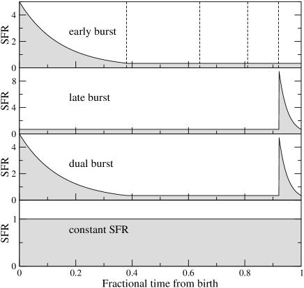
Four different SFH types were considered. These were chosen to establish how the reconstruction fares with the presence/absence of early and/or late star formation activity. The four SFH types are:

• Early burst - The early burst SFH starts with a high SFR from the moment the galaxy is born followed by an exponential decay. After approximately 40% of the galaxy’s age, the decay ceases leaving a small SFR that remains constant for the remainder of the galaxy’s history.

• Late burst - This SFH has a small constant SFR from birth up until approximately 90% of the galaxy’s age. At this point, it undergoes an instantaneous burst which exponentially decays back to the small constant SFR the galaxy experienced prior to the burst.

• Dual burst - This is the early burst SFH with the last 10% of the history replaced with the late busrst SFH.

• Constant SFR - The SFR is constant throughout the entire history for this SFH.

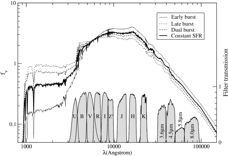
The different SFHs are plotted in Figure 1 with a SFR scale that corresponds to the creation of 1M_⊙ over the history of the galaxy. Absolute SFRs for each galaxy are determined by normalising to the absolute $R$ band magnitude as described below. The early and late bursts are designed to fit entirely within their respective early and late SFH blocks used for re-binning in Section 4 (see Figure 1). Although the early burst creates approximately four times the stellar mass created in the late burst, the bolometric luminosity of the late burst is ten times that of the early burst. Figure 2 plots the SED corresponding to each SFH type.

Figure 1: The four different SFHs used in the creation of the synthetic galaxy catalogues. The fractional time runs from the big bang to the epoch at the galaxy’s redshift. The dashed lines in the top panel indicate the blocks within which all reconstructed SFHs are re-sampled. The early and late bursts are designed to fit entirely within the first and last of these blocks respectively. The bolometric luminosity of the early burst is approximately one tenth that of the late burst.

For every SFH type, four galaxy catalogues were generated, each using one of the following filtersets:

• Full set – $U$, $B$, $V$, $R$, $I$, $Z^{\prime}$, $J$, $H$, $K$, $3.6\mu$m, $4.5\mu$m, $5.8\mu$m and $8\mu$m. The full set contains all 13 broad band filters considered in this paper. The last four bands are those of the Infra Red Array Camera (IRAC) on board the Spitzer Space Telescope.

• Half set – $B$, $R$, $I$, $J$, $K$, $3.6\mu$m and $4.5\mu$m. The half set spans a slightly narrower range of wavelengths than that spanned by the full set and contains half the number of filters. This set also omits the 5.8 and 8$\mu$m IRAC bands which are in practice dominated by dust and PAHs.

• Optical set – $U$, $V$, $R$, $I$, $Z^{\prime}$. This set is included to match the set of filters used by the SDSS.

• Infra-red set – $Z^{\prime}$, $J$, $H$, $K$, $3.6\mu$m and $4.5\mu$m. This set is purely to assess how well infra-red data fares without optical band photometry.

The filter transmission curves are plotted in Figure 2 for comparison with the four different SFH type SEDs.

Figure 2: Synthetic SEDs corresponding to the early burst, late burst, dual burst and constant SFR histories (see Figure 1) for a galaxy at $z=0$ and with $Z=0.1Z_{\odot}$, $A_{V}=0$. SEDs are plotted normalised to the same $R$ band flux. The filter transmission efficiency is shown for comparison and is correctly scaled. The total throughput in each passband is given by scaling all filters by an additional global system efficiency of 70% (see text). Left ordinate is plotted on a log scale and applies to the SEDs, right ordinate is linear and applies to the filter curves.

Each of the 16 catalogues was populated with 1000 galaxies with random redshifts, metallicities and extinctions. For each galaxy, apparent magnitudes were generated following these steps:

• Assign a random absolute $R$ band magnitude distributed according to the $R$ band luminosity function of Wolf et al. (2003) described by a Schechter function (Schechter, 1976) with parameters $M_{*}=-20.70+5{\rm lg\,h_{0}}$, $\alpha=-1.60$.

• Assign a random redshift drawn from the probability distribution function $z\,\,{\rm exp}\,(-z^{2}/4)$ within the range $0<z<6$.

• Assign a random extinction drawn from a uniform distribution within the range $0<A_{V}<3$.

• Assign a random metallicity from a uniform logarithmic distribution within the range $0.005<Z/Z_{\odot}<2.5$. (Note that this work assumes mono-metallic SFHs, i.e., $Z$ is held constant over the galaxy’s entire history. See Section 5). Linear interpolation in log($Z$) between the discrete metallicity library SEDs ensures a continuous distribution in $Z$.

• Compute the apparent $R$ band magnitude using $z$, the absolute $R$ band magnitude from step 1) and the K-correction from the appropriate synthetic SED.

• Compute fluxes in all passbands using the appropriate redshifted, reddened but arbitrarily scaled synthetic SED.

• Normalise each passband flux by the factor needed to scale the $R$ band flux computed in step 6) to the apparent $R$ band magnitude computed in step 5). Fluxes at this point are in units of photons/s/m².

• Assuming a telescope collecting area of 64m² for filters $U$ to $K$ and 0.6m² for the four IRAC bands, an integration time of 1800s per filter and an overall system efficiency of 70% in all filters, compute Poisson errors for each flux.

• Scatter fluxes by their errors computed in step eight then convert the resulting fluxes and their errors to AB mags.

Once the photometry is computed for a given source in this way, the number of filters with non-detections, defined by a flux significance of $<10\sigma$, are counted. Sources that are not detected in at least 70% or five (whichever is larger) of the filters contained within the set are rejected. Sampling continues in this way until 1000 objects have been generated for the catalogue. The 1800s exposure per filter and telescope collecting area assumed in step eight above correspond to the following 10$\sigma$ magnitude sensitivity limits: 26.5, 25.9, 25.6, 25.0, 24.8, 23.9, 22.8, 22.2, 22.6, 24.1, 23.5, 21.4, 21.3 in $U$, $B$, $V$, $R$, $I$, $Z^{\prime}$, $J$, $H$, $K$, $3.6\mu$m, $4.5\mu$m, $5.8\mu$m and $8\mu$m respectively. Non-detections are assigned an apparent magnitude equal to the sensitivity limit of the corresponding filter and an error of 0.5 mag. The system efficiency assumed in step 8) applies in addition to the absolute filter transmission efficiencies indicated in Figure 2 (this brings the IRAC filters to the correct total passband throughputs and accommodates typical optical and IR camera throughputs).

Figure 3: An example of the variation of apparent $R$ band magnitude with redshift for all objects in one of the early burst catalogues. The continuous line shows how $R$ varies with redshift for a M=-22.0 early burst galaxy with $Z=0.1Z_{\odot}$ and $A_{V}$=0. The dashed lines indicate bins within which objects were selected for the analyses of Section 4.2. The magnitude bin $24<R<25$ selects objects with an approximately constant photometric S/N over as large a range in redshift as possible, whilst the redshift bin $1<z<2$ optimises both the number of objects and their S/N range.

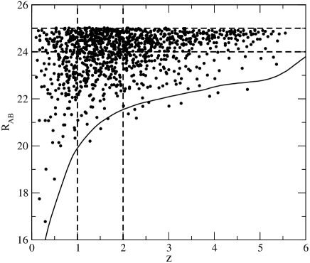
In Section 4.2 the effect of photometric S/N and redshift on the reconstructed SFHs and stellar masses is investigated. Two catalogue sub-sets were therefore defined to achieve this. To test dependency on S/N with as little variation in redshift as possible, sources within $1<z<2$ were selected. To test dependency on as large a range in redshift as possible at approximately the same S/N, sources were selected within $24<R<25$. These sub-sets are shown in Figure 3 where the apparent $R$ band magnitude is plotted against $z$ for 1000 sources generated using the early burst SFH.

4 Simulation results

This section discusses application of the SFH reconstruction method to synthetic catalogues to assess its performance. An initial demonstration of setting the optimal regularisation is given in Section 4.1 before applying the method to the full range of catalogues in Section 4.2.

4.1 The effect of regularisation

The effect of regularisation is demonstrated with an example. Using the late burst SFH, synthetic photometry was generated in the full filterset for a galaxy at $z=1$ with absolute $R$ band magnitude $M_{R}=-20$, $A_{V}=0$ and $Z=0.1Z_{\odot}$. The resulting stellar mass of the galaxy was $9.7\times 10^{9}\,{\rm M}_{\odot}$. The SFH reconstruction method was then applied for different degrees of regularisation. In each case, the SFH was divided into five exponentially spaced blocks as indicated in the top panel of Figure 1 (see Section 2.3). For comparison with the reconstructed SFHs, the input SFH was binned into the same five exponentially spaced blocks.

Figure 4: Demonstration of the effect of different regularisation weights, $w$, on the reconstructed SFH. This example is based on a synthetic source lying at $z=1$ with $Z=0.1Z_{\odot}$, $M_{R}=-20$ and $A_{V}=0$. The reconstruction uses the full set of 13 filters. The input SFH is the late burst model shown here by the thick grey dashed line, binned into five SFH blocks. The optimal regularisation weight found by maximising the Bayesian evidence produces the most accurate reconstructed SFH (continuous line). Under-regularisation (dot-dashed line) results in a very inaccurate SFH reconstruction whereas over-regularisation (thin dashed line) smooths the SFH too heavily. For clarity, the standard errors returned by equation (11) are shown only for the optimally regularised case. In all cases, the points are placed at the SFH block centres.

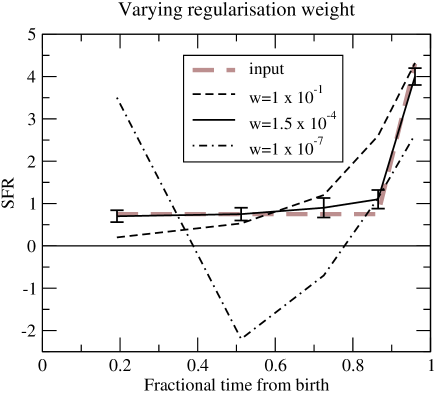
Figure 4 shows how accurately the input late burst SFH was reconstructed with three different values of the regularisation weight, $w$. One of these values is the optimal weight, $w=1.5\times 10^{-4}$, as determined by the maximal evidence, whilst the remaining two were set higher and lower than this by $\sim 3$ dex. In the figure, the input binned SFH is shown by the heavy dashed line. Clearly, the optimal regularisation weight gives the most accurate reconstruction. Over-regularisation smooths the SFH too heavily, leading to a biased reconstructed SFH. Conversely, under-regularisation gives rise to a catastrophic failure, with the SFH ringing violently about the input SFH.

The exercise also serves to demonstrate that the reconstructed stellar mass (computed using equation 6) depends on $w$. Comparing with the stellar mass of the input galaxy of $9.7\times 10^{9}\,{\rm M}_{\odot}$, the optimally regularised case recovered a mass of $(9.9\pm 0.3)\times 10^{9}\,{\rm M}_{\odot}$, the under-regularised case recovered $(1.61\pm 0.06)\times 10^{10}\,{\rm M}_{\odot}$ and the over-regularised case recovered $(8.9\pm 0.2)\times 10^{9}\,{\rm M}_{\odot}$. A sub-optimal regularisation weight can therefore bias the reconstructed mass.

As stated previously, the actual number of SFH blocks is always higher than the effective number of blocks when regularising due to the smoothness constraints imposed on the SFH. To reiterate, this is why the evidence should be the statistic used to rank models rather than $\chi^{2}$. These constraints increase the covariance between pairs of SFH blocks although the effect is counteracted by the evidence which selects fewer SFH blocks (and hence less covariant solutions) when the data do not support a high resolution SFH. Inspection of many realisations of the covariance matrix (excluding failed reconstructions – see next section) indicates that highly covariant solutions do not occur. A further observation is that the early blocks are always more covariant than the later blocks.

4.2 Application to the full suite of catalogues

The SFH reconstruction method was applied to the full suite of catalogues. An assessment was made of how the accuracy of the reconstructed SFH depends on the number of filters, the wavelength range spanned by the filterset, the S/N of the photometry, the presence and/or absence of early and/or late star formation activity and redshift. For each combination of these variables, a synthetic catalogue was generated, comprising 1000 galaxies adhering to the ranges in $z$, $A_{V}$, $Z$ and absolute magnitude given in Section 3. For every object in each case, the SFH was reconstructed following the procedure outlined in Section 2.3, maximising the evidence by varying the regularisation weight, number of SFH blocks and metallicity.

Figure 5: SFH reconstruction binned by redshift as labelled. SFH type is separated by column and filterset by row. Reconstructed SFHs are shown by the data points and lines (staggered for clarity) and apply to objects selected by $24<R<25$. Error bars show the standard deviation of objects in the redshift bin. Grey shaded histograms are the binned input SFHs.

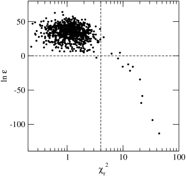
The results show that approximately 1% of reconstructions completely fail to recover the input SFH or galaxy parameters. The size of this fraction is independent of SFH type or filterset. These catastrophic failures occur either when the maximisation becomes stuck at an incorrect local maximum or when the maximisation fails to converge. Fortunately, these cases are easily identified by their very small evidence and large $\chi^{2}$. Figure 6 shows the distribution of sources in the ln$\,\epsilon$, $\chi^{2}$ plane for the early burst SFH and full filterset reconstruction (see next section). The catastrophic failures form the long tail extending to low $\epsilon$ and high $\chi^{2}$ and can be discounted by retaining only objects with ln$\,\epsilon>0$ and $\chi_{r}^{2}<4$. In all analyses hereafter, this cut has been applied. The figure also serves to illustrate that there is not a clear relationship between the evidence and $\chi^{2}$, i.e., minimising $\chi^{2}$ is by no means equivalent to minimising $-{\rm ln}\,\epsilon$.

Figure 6: Distribution of 1000 reconstructions in the plane spanned by log-evidence and reduced $\chi^{2}$ for the early burst SFH and full filterset. Catastrophic failures lie in the tail extending to low $\epsilon$ and high $\chi_{r}^{2}$ and are removed in all analyses in this paper using the limits ln$\,\epsilon>0$ and $\chi_{r}^{2}<4$ indicated by the dashed lines.

4.2.1 Dependence on filterset and SFH type

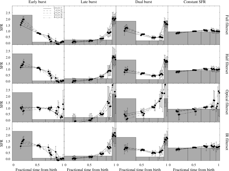
Figure 5 shows how the method performs as a function of SFH type, filterset and redshift. Each panel corresponds to a different combination of SFH type and filterset and in every panel, the average reconstructed SFH and its standard deviation is plotted for sources in five different redshift bins: $0<z<1$, $1<z<2$, $2<z<3$, $3<z<4$ and $4<z<6$. To allow for variation in the number of preferred SFH blocks from source to source, each reconstructed SFH was finely sampled with a small fixed time step then re-binned to a common five-block SFH. An effect of the re-binning is to smear the reconstructed SFHs slightly, particularly when re-binning from a lower number of blocks. However, comparing with SFHs averaged over only those sources preferring five bins shows that this effect is relatively minor with no more than five per cent of the total stellar mass being smeared between any pair of bins in all cases.

The results plotted in Figure 5 illustrate that the SFH type and filterset have a strong influence on the accuracy with which the input SFH can be recovered. In terms of the filters, the full set unsurprisingly performs best. However, a mildly surprising find is that the half set gives very similar average SFHs, albeit with $\sim 30\%$ larger scatter on average. Clearly, the wavelength range spanned by the filterset is the important factor, rather than the existence of an extra six intermediate photometric points provided by the full set. Furthermore, the IR end of the filterset is more important than the optical end, as indicated by the bottom two rows of Figure 5. The optical SDSS-like set performs poorly, significantly worse than the IR set. Only in the specific case of the late burst does the SFH reconstructed using optical photometry consistently resemble the input SFH, but this can not be reliably distinguished from the other cases.

In terms of the SFH type, the late burst and constant SFHs are reconstructed the most faithfully although the late burst is smeared slightly towards earlier times. The early burst reconstructions are more strongly smeared over the first few bins, giving rise to less star formation at early times and more during their mid-history than actually occurred. On average, $\sim 20\%$ of the stellar mass created in the early burst is smeared into the later blocks. The stronger smearing exhibited by the early burst is a result of its bolometric luminosity being ten times smaller than that of the late burst. Nevertheless, the reconstructed SFHs still prove a useful diagnostic for the presence of early star formation activity, showing a clear excess that declines with time to accurately reproduce the latest SFR (with the exception of the optical filterset which fails to recover a decline at all redshifts). The dual burst proves the most challenging of SFH types to reconstruct. In this case, the full and half filtersets best recover the early and late bursts, implying the necessity of both optical and IR filters, although sources at $z<1$ have more strongly smeared SFHs. Again, this demonstrates the importance of the IR filters.

Figure 7: SFH reconstruction binned by magnitude as labelled. SFH type is separated by column and filterset by row. Reconstructed SFHs are shown by the data points and lines (staggered for clarity) and apply to objects selected by $1<z<2$. Error bars show the standard deviation of objects in the redshift bin. Grey shaded histograms are the binned input SFHs.

Note that the effect of regularisation on the average of a sample of SFHs is twofold. A stronger regularisation weight reduces the scatter in the sample, whilst more heavily smoothing the average SFH. This effect can be seen to an extent by comparing the reconstructed early burst SFH for the full and half filtersets in Figure 5. The error bars on points in the first bin with the half filterset are of equal size or smaller than the error bars of the first bin with the full set. However, the SFHs are more heavily smeared with the half set.

4.2.2 Dependence on S/N and redshift

Figure 5 shows that in nearly all cases, the variation in reconstructed SFHs between different redshift bins is comparable to or less than the intrinsic SFH scatter within a given bin. Generally, the low redshift sources (selected by say $z<2$) tend to have more smeared SFHs than their higher redshift equivalents. This is consistent with the fact that at $z\mathbin{\lower 3.0pt\hbox{$\hbox to0.0pt{\raise 4.0pt\hbox{$\char 62\relax$}\hss}\mathchar 29208\relax$}}2$, the rest-frame UV is redshifted into the optical wavebands where SEDs are much more sensitive to stellar age (see Figure 2 – note that the optical filterset performs worst despite this since it lacks the SED normalisation provided by the IR filters). Furthermore, since the SFHs in Figure 5 are computed for sources selected by $24<R<25$ (i.e., they have approximately the same photometric S/N), the flux received by the IRAC filters increases with redshift, providing more discrimination at the IR end of the SED.

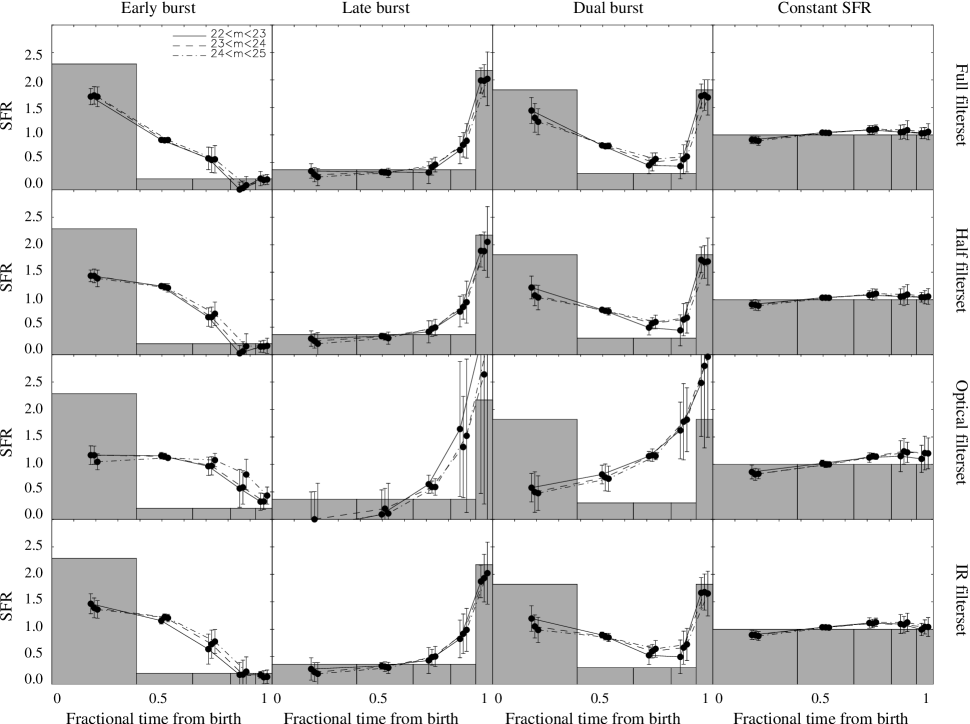
Figure 7 shows reconstructed SFHs for the different combinations of filterset and SFH type, but this time objects are binned by apparent magnitude. All objects are selected by $1<z<2$ to maximise the number of objects whilst maintaining a large span in apparent magnitude and thus S/N. As the figure shows, there is little variation with S/N. The averaged SFHs are very similar, although unsurprisingly, the scatter increases as the apparent magnitude falls.

As can be inferred from Figures 5 and 7, the reconstructed SFH can give rise to negative SFRs. This is especially true of the inadequate optical filterset. With the other three filtersets, negative SFRs still occur but such cases; 1) tend to be limited to galaxies with low S/N photometry, 2) are always consistent with a null SFR, 3) are relatively infrequent due to the optimal regularisation strength selected by the evidence.

4.2.3 Recovery of stellar mass and metallicity

Figure 8: Accuracy of reconstructed mass. Each panel corresponds to a different filterset as labelled. For each filterset, the reconstructed mass is plotted against the input mass for the early burst SFH, late burst SFH (reconstructed mass $\times 10$), dual burst SFH (reconstructed mass $\times 100$) and constant SFR (reconstructed mass $\times 1000$). Tables in the bottom right of each panel list the fractional scatter $\left<({\rm M}_{\rm recon}-{\rm M}_{\rm input})^{2}/{\rm M}_{\rm input}^{2}\right>^{1/2}$ and the bias $\left<({\rm M}_{\rm recon}-{\rm M}_{\rm input})/{\rm M}_{\rm input}\right>$ for the different SFH types.

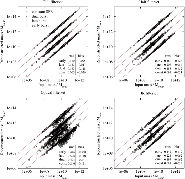
Figure 8 shows the recovered stellar mass as a function of the input mass for the different combinations of SFH type and filter set. In the lower right hand corner of each panel, a table lists the fractional scatter $\left<({\rm M}_{\rm recon}-{\rm M}_{\rm input})^{2}/{\rm M}_{\rm input}^{2}\right>^{1/2}$ and the bias $\left<({\rm M}_{\rm recon}-{\rm M}_{\rm input})/{\rm M}_{\rm input}\right>$ for each SFH type.

As expected, the full filterset recovers the stellar mass most accurately (smallest bias) and with the least scatter. However, all cases show a negative bias such that the recovered mass is on average less than the input mass. For the full filterset, this bias ranges from $\sim 3\%$ for the constant SFR to $\sim 13\%$ for the dual burst SFH. The largest bias of $\sim 40\%$ occurs with the early burst SFH and optical filterset. However, in all cases, the bias is less than the fractional scatter.

Compared with the full filterset reconstructions, the half set again performs very well given the reduction from 13 filters to seven. The fractional scatter of the half set is higher than that of the full set by $\sim 25\%$ on average. Similarly, the IR filterset results in an increased fractional scatter of only $\sim 30\%$ compared to the full set on average. The optical filterset gives a significantly larger scatter of around four times that of the full set or three times the IR set on average, confirming the well known fact that IR photometry is essential for the accurate measurement of stellar mass.

In terms of the dependence of mass recovery on SFH type, the constant SFR masses show the smallest bias, closely followed by those of the late burst (although the late burst gives rise to significantly more scatter). The early burst masses tend to be more accurately reconstructed than the late burst or dual burst masses, especially in the case of the IR filterset where they are recovered almost as accurately as the full filterset case. This demonstrates the importance of IR filters for measuring stellar mass created in early bursts.

Figure 9: Accuracy of reconstructed metallicity. Each panel corresponds to a different filterset as labelled. For each filterset, the recovered metallicity is plotted against the input metallicity for the early burst SFH, late burst SFH (reconstructed $Z$ $\times 10^{2}$), dual burst SFH (reconstructed $Z$ $\times 10^{4}$) and constant SFR (reconstructed $Z$ $\times 10^{6}$). Tables in the bottom right of each panel list the fractional scatter $\left<(Z_{\rm recon}-Z_{\rm input})^{2}/Z_{\rm input}^{2}\right>^{1/2}$ and the bias $\left<(Z_{\rm recon}-Z_{\rm input})/Z_{\rm input}\right>$ for the different SFH types.

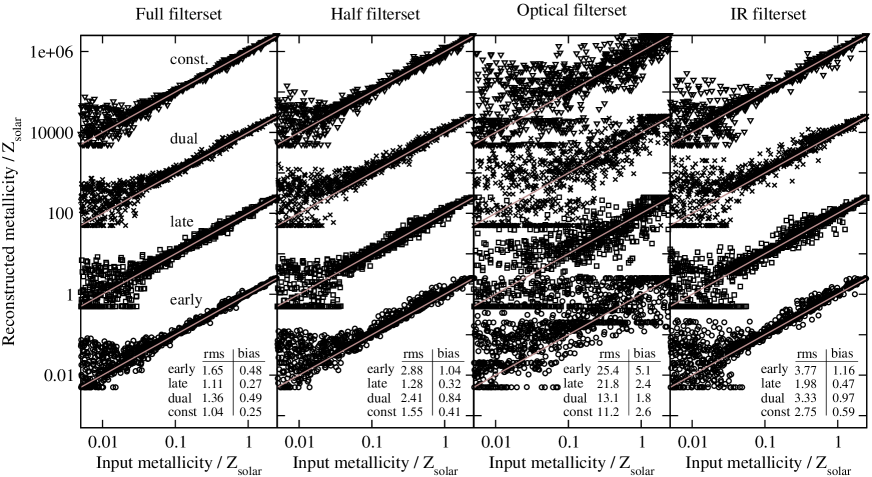
Figure 9 plots the recovered metallicity as a function of the input metallicity for all SFH types and filtersets. The scatter in the recovered metallicity, particularly at low $Z$ ($<0.1Z_{\odot}$), is larger than the scatter seen in the reconstructed mass but the global trends are essentially the same. The full filterset recovers metallicity most accurately, the half filterset and IR filterset having a scatter larger by $\sim 60\%$ and $\sim 120\%$ respectively on average. The very large scatter exhibited by the optical filterset demonstrates that recovery of metallicity without IR filters is extremely unreliable. In all cases, the recovered metallicity is larger than the input value, although similar to the recovered mass, this bias is always significantly lower than the scatter.

4.2.4 SFH resolution

In the previous sections, SFHs were re-binned to bring them to a common resolution of five blocks to enable comparison between reconstructions. In this section, dependency of the reconstructed SFH resolution (i.e., number of blocks, $N_{\rm block}$) on data quality, SFH type and filterset is considered.

Figure 10: Distribution of the optimal number of SFH blocks, $N_{\rm block}$, chosen by the Bayesian evidence for different redshift and magnitude selections, SFHs and filtersets. The reference selection shown by the unshaded histogram in each panel satisfies the criteria $1<z<2$ and $R>24$ with the full filterset and early burst SFH.

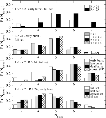
Figure 10 shows how the distribution of $N_{\rm block}$ varies as the data vary. The top panel shows that higher S/N data allow a higher SFH resolution, sources selected by $R<23$ preferring five to six blocks on average, compared with $R>24$ sources preferring an average of four to five blocks. The panel second from top shows how the resolution varies as a function of redshift for sources of approximately constant S/N ($R>24$). The differences are not significant, with sources across all redshifts preferring five bins on average.

The third panel from top in Figure 10 shows how the SFH resolution depends on SFH type. In this case, there are more significant differences. The late burst, dual burst and constant SFR histories allow a higher resolution of six blocks on average, compared to the early burst of five. Finally, the bottom panel shows the dependence of resolution on filter set. Unsurprisingly, the full set allows the highest resolution on average, with the majority of galaxies preferring four or five SFH blocks. In comparison, the distribution in resolution of the reduced filtersets is skewed to lower numbers of SFH blocks, particularly the IR set.

Clearly, there is a degeneracy between the SFH resolution and the regularisation weight, since a higher level of regularisation acts to smooth the SFH, effectively reducing its resolution. In Figure 11, two example confidence regions are shown in the plane spanned by regularisation weight and $N_{\rm block}$ computed from the Bayesian evidence. The heavy contours correspond to the late burst SFH and the thin contours the early burst SFH for a $z=1$, $Z=0.1Z_{\odot}$, $M_{R}=-18$ and $A_{V}=0$ galaxy. The inclination of both contours shows that this degeneracy does indeed exist. However, the degeneracy is weak and therefore locating the maximum in the evidence distribution is relatively straightforward.

Figure 10 illustrates that the number of SFH blocks that can be recovered on average is comparable to the typical number recovered by Tojeiro et al. (2007) from optical spectra. However, there are two major differences with the present study that make this an unfair comparison. These are that mono-metallic populations are considered and that filtersets extend to the IR. Increasing the number of parameters to describe a time-varying metallicity will reduce the number of SFH blocks that can be recovered (see Section 5). Similarly, the IR filters provide extra constraints on the SFH, allowing reconstruction at a slightly higher resolution. As Figure 10 shows (for the early burst, but this applies generally), the full filterset recovers more SFH blocks on average than the optical set even though the optical set is similar but lacking the IR bands.

Figure 11: Confidence limits on regularisation weight, $w$, and number of SFH blocks, $N_{\rm block}$ for a $z=1$, $Z=0.1Z_{\odot}$, $M_{R}=-18$ and $A_{V}=0$ galaxy generated using the early burst SFH (thin contours) and late burst SFH(thick contours). Contours are computed from the evidence and correspond to 68%, 95.4% and 99.7% confidence levels.

5 Summary

The primary aim of this study has been to assess reconstruction of discretised SFHs using a new method applied to multi-band photometric data. Although not tested in this paper, the method can also be applied to spectroscopic data as well as a mixture of both spectroscopic and multi-band data.

The method differs from existing methods by maximising the Bayesian evidence instead of minimising $\chi^{2}$ (or maximising the posterior probability). For regularised solutions, the evidence gives the unbiased relative probability of the fit between different model parameterisations. This is unlike the $\chi^{2}$ statistic which suffers from an ambiguous number of degrees of freedom that changes between parameterisations when regularisation is applied.

This work has demonstrated that the evidence allows the data to correctly and simultaneously set the optimal regularisation strength and the appropriate number of blocks in the reconstructed SFH. Although negative SFRs can arise, the optimal level of regularisation ensures that the fraction of such cases is low. Negative SFRs are limited mainly to galaxies with low photometric S/N and inadequate filter sets (e.g., the optical set considered in this work). Provided the filter set is adequate, negative SFRs are always consistent with a null SFR. This approach may be preferable to schemes that enforce positive SFRs. Enforcing positivity not only risks artificial ringing and biasing in the reconstructed SFH, it also hides problems that give rise to negative SFRs.

Application of the method to a range of synthetic galaxy catalogues generated with varying passband sets and SFHs demonstrates that use of multi-band data in constraining SFHs is feasible along with certain caveats. The scatter seen in the SFHs reconstructed in this work shows that occasional significant inaccuracies can occur even with a comprehensive filterset that extends up to near-IR and mid-IR wavelengths. Therefore, interpretation of SFHs recovered from solely multi-band photometry on a galaxy by galaxy basis should be conducted with some caution. The mean SFH of a sample of galaxies is therefore a more reliable quantity in order to average out uncertainties although this study indicates that averaging over only four galaxies readily allows a late burst to be distinguished from an early burst. In comparison, studies using spectroscopic data show that reliable SFHs can be derived for individual galaxies. Nevertheless, multi-band photometry allows reconstruction of SFHs for many times more galaxies than spectroscopic methods for the same amount of observing time.

The most important factor governing the accuracy of the reconstructed SFHs is the wavelength range spanned by the filterset. The results show little difference between two filtersets that span approximately the same wavelength range (optical to mid-IR) despite one set having half the number of filters of the other. Conversely, SFHs based on only purely optical photometry are completely unreliable, it being impossible to distinguish any of the input SFHs investigated. A filterset consisting of only near and mid IR filters ($Z^{\prime}$ – 4.5$\mu$m) allows recovery of SFHs to within a comparable accuracy to that recovered when optical filters are also included, implying that the majority of the SFH constraints are provided by near and mid-IR data (for the SFHs tested here).

In terms of the ability of multi-band photometry to constrain different SFH types, the results show that apart from the case where only optical filters are used, early bursts of star formation can be differentiated from late bursts and both of these can be distinguished from dual bursts and constant SFRs. However, early bouts of star formation activity are always artificially smeared to later times in the reconstructed SFH compared to the input SFH. These findings apply specifically to the SFHs considered in this work, where the early burst gives rise to bolometric luminosity that is one tenth that of the late burst. A quick test has revealed that a stronger early burst is more accurately recovered with less smearing to late times. In addition, although the dual burst SFH used here suggests that recovery of more than two bursts would be unfeasible with the filtersets tested, bursts with more similar bolometric luminosities can be more readily recovered. This was demonstrated by Ocvirk et al. (2006) who showed that CSP SEDs constructed from flux normalised bursts allow a higher SFH resolution on average than SEDs constructed from mass normalised bursts.

The results presented in this paper have been obtained using the Bruzual & Charlot (2003) spectral libraries. Whilst the exact values of the numerical results quoted here will depend on the specific SED library of choice, there are no compelling reasons to suggest that the observed trends would not remain valid generally.

This study has considered a specific case where galaxy redshift and extinction are known prior to reconstructing the SFH. Also, mono-metallic stellar populations have been assumed where the metallicity does not evolve as the galaxy ages. Clearly, the more general problem necessitates maximising the evidence over extra parameters. The expected effect of this is that the maximum evidence would shift to lower SFH resolutions on average. Although generalising to a variable redshift and extinction is a relatively small expansion of the non-linear parameter space, incorporating a time-varying metallicity in addition results in a significantly larger and more complex non-linear parameter space. This increases the time required to locate the maximum evidence and increases the risk of becoming trapped at a local maximum.

However, there are two small reprieves. The first is that the metallicity history can be regularised in a similar manner to the SFH, smoothing the evidence surface and therefore easing maximisation. The second exploits SED libraries with discrete metallicities. As shown by Tojeiro et al. (2007), finding the optimal metallicity within the range spanned by two tabulated values of metallicity is also a linear problem which can be directly combined with the linear inversion of the SFH. In this way, optimising the metallicity for each SFH block reduces to searching a smaller number of discrete values. A full investigation of the general case will be presented in forthcoming work.

Appendix A Ranking models by Bayesian evidence

In this appendix, the theory of Suyu et al. (2006) is applied to the present problem. Using the notation in Section 2.2, Bayes’ theorem states that the posterior probability of the parameters $\mathbf{a}$ given the data $\mathbf{d}$, model $\mathbf{G}$ and regularisation ($\mathbf{H},w$) can be expressed as

$$P(\mathbf{a}|\mathbf{d},\mathbf{G},\mathbf{H},w)=\frac{P(\mathbf{d}|\mathbf{a},\mathbf{G})P(\mathbf{a}|\mathbf{H},w)}{P(\mathbf{d}|\mathbf{G},\mathbf{H},w)}\,.$$ (16)

Here, $P(\mathbf{d}|\mathbf{a},\mathbf{G})$ is the likelihood which gives the probability of the data given the model parameters, $P(\mathbf{a}|\mathbf{H},w)$ is the prior which forces an a priori assumption on the parameters $\mathbf{a}$ given some regularisation model and $P(\mathbf{d}|\mathbf{G},\mathbf{H},w)$ is a normalisation term called the evidence.

In the first level of inference where the most likely parameters $\mathbf{a}$ are determined, the evidence is constant and therefore plays no part. The evidence becomes relevant in the higher levels. For example, in the second level where one wishes to find the optimal regularisation weight, $w$, Bayes’ theorem shows that the following posterior probability must be maximised:

$$P(w|\mathbf{d},\mathbf{G},\mathbf{H})=\frac{P(\mathbf{d}|\mathbf{G},\mathbf{H},w)P(w)}{P(\mathbf{d}|\mathbf{G},\mathbf{H})}\,.$$ (17)

The first term in the numerator of this equation is the evidence in equation (16).

In the third level of inference where different models and regularisation types are ranked, the posterior probability, again using Bayes’ theorem can be written

$$P(\mathbf{G},\mathbf{H}|\mathbf{d})\propto P(\mathbf{d}|\mathbf{G},\mathbf{H})P(\mathbf{G},\mathbf{H})\,.$$ (18)

With a flat prior $P(\mathbf{G},\mathbf{H})$, the likelihood $P(\mathbf{d}|\mathbf{G},\mathbf{H})$ can be used to rank the data. The likelihood can be written

$$P(\mathbf{d}|\mathbf{G},\mathbf{H})=\int P(\mathbf{d}|\mathbf{G},\mathbf{H},w)P(w){\rm d}w$$ (19)

where, again, $P(\mathbf{d}|\mathbf{G},\mathbf{H},w)$ is the evidence in equation (16). As Suyu et al. (2006) discuss, a reasonable approximation is to treat $P(w)$ as a delta function centred on the optimal regularisation weight, $\hat{w}$, since $\hat{w}$ has a well defined value estimable from the data. In this case, with a flat prior $P(\mathbf{G},\mathbf{H})$, the model ranking posterior probability given by equation (18) is simply equal to the value of the evidence at $\hat{w}$. The most probable model ($\mathbf{G},\mathbf{H}$) is therefore found by maximising the evidence at $\hat{w}$.

Acknowledgements

SD is supported by the Particle Physics and Astronomy Research Council and thanks Steve Eales and Luca Cortese for helpful discussion.

References

- Benitez (2000) Benitez, N., 2000, ApJ, 536,571
- Bertelli et al. (1994) Bertelli, G., Bressan, A., Bertelli, G., Chiosi, C., Fagotto, F., Nasi, E., 1994, A&AS, 106, 275
- Bertin & Arnouts (1996) Bertin, E. & Arnouts, S., 1996, A&AS, 117, 393
- Borch et al. (2006) Borch, A., Meisenheimer, K., Bell, E. F., Rix, H.-W., Wolf, C., Dye, S., Kleinheinrich, M., Kovacs, Z., Wisotzki, L., 2006, A&A, 453, 869
- Bruzual & Charlot (2003) Bruzual, G. & Charlot, S., 2003, MNRAS, 344, 1000
- Calzetti et al. (2000) Calzetti, D., Armus, L., Bohlin, R. C., Kinney, A. L., Koorneef J., Storchi-Bermann, T., 2000, ApJ, 533, 682
- Chilingarian et al. (2007) Chilingarian, I., Prugniel, P., Sil’Chenko, O., Koleva, M., 2007, IAUS, 241, 175
- Cid Fernandes et al. (2004) Cid Fernandes, R., Gu, Q., Melnick, K., Terlevich, E., Terlevich, R., Kunth, D., Rodrigues Lacerda, R., Joguet, B., 2004, MNRAS, 355, 273
- Cid Fernandes et al. (2005) Cid Fernandes, R., Mateus, A., Sodré Jr., L., Stasińska, G., Gomes, J. M., 2005, MNRAS, 358, 363
- Cid Fernandes et al. (2007) Cid Fernandes, R., Asari, N. V., Sodré Jr., L., Stasińska, G., Mateus, A., Torres-Papaqui, J. P., Schoenell, W., 2007, MNRAS, 375, L16
- Dye & Warren (2005) Dye, S. & Warren, S. J., 2005, ApJ, 623, 31
- Dye et al. (2007) Dye, S., Smail, I., Swinbank, A. M., Ebeling, H., Edge, A. C., 2007, MNRAS, 379, 308
- Dye et al. (2008) Dye, S., Evans, N. W., Belokurov, V., Warren, S. J., Hewett, P., 2008, MNRAS submitted
- Gavazzi et al. (2002) Gavazzi, G., Bonfanti, C., Sanvito, G., Boselli, A., Scodeggio, M., 2002, ApJ, 576, 135
- Heavens, Jimenez & Lahav (2000) Heavens, A. F., Jimenez, R. & Lahav, O., 2000, MNRAS, 317, 965
- Heavens et al. (2004) Heavens, A. F., Panter, B., Jimenez, R., Dunlop, J., 2004, Nature, 428, 625
- Kauffmann et al. (2003) Kauffmann, G., et al., 2003, MNRAS, 341, 33
- Kaviraj et al. (2007) Kaviraj, S., et al., 2007, ApJS, 173, 619
- Koleva et al. (2008) Koleva, M., Prugniel, P., Ocvirk, O., Le Borgne, D., Soubiran, C., 2008, MNRAS, in press, arXiv0801.0871
- MacKay (2003) MacKay, D. J. C., Information Theory, Inference and Learning Algorithms, Cambridge University Press
- Noeske et al. (2007) Noeske, K. G., et al., 2007, ApJ, 660, L47
- Nolan et al. (2006) Nolan, L. A., Harva, M. O., Kabán, A., Raychaudhury, S., 2006, MNRAS, 366, 321
- Nolan et al. (2007) Nolan, L. A., Dunlop, J. S., Panter, B., Jimenez, Raul, Heavens, A., Smith, G., 2007, MNRAS, 375, 371
- Ocvirk et al. (2006) Ocvirk, P., Pichon, C., Lançon, A., Thiébaut, E., 2006, MNRAS, 365, 46
- Panter, Heavens & Jimenez (2003) Panter, B., Heavens, A. F. & Jimenez, R., 2003, MNRAS, 343, 1145
- Panter, Heavens & Jimenez (2004) Panter, B., Heavens, A. F. & Jimenez, R., 2004, MNRAS, 355, 764
- Panter et al. (2007) Panter, B., Jimenez, R., Heavens, A. F., Charlot, S., 2007, MNRAS, 378, 1550
- Reichardt, Jimenez & Heavens (2001) Reichardt, C., Jimenez, R., Heavens, A. F., 2001, MNRAS, 327, 849
- Salim et al. (2007) Salim, S., et al., 2007, ApJS, 173, 67
- Salpeter (1955) Salpeter, E. E., 1955, ApJ, 121, 161
- Schawinski et al. (2007) Schawinski, K., Thomas, D., Sarzi, M., Maraston, C., Kaviraj, S., Joo, S. -J., Yi, S. K., Silk, J., 2007, MNRAS, 382, 1415
- Schechter (1976) Schechter, P., 1976, ApJ, 203, 297
- Sheth et al. (2006) Sheth, R. K., Jimenez, R., Panter, B., Heavens, A. F., 2006, ApJ, 650, 25
- Stoughton et al. (2002) Stoughton, C., et al., 2002, AJ, 123, 485
- Suyu et al. (2006) Suyu, S. H., Marshall, P. J., Hobson, M. P., Blandford, R. D., 2006, MNRAS, 371, 983
- Tojeiro et al. (2007) Tojeiro, R., Heavens, A. F., Jimenez, R., Panter, B., 2007, MNRAS, 381, 1252
- Vergeley, Lançon & Mouhcine (2002) Vergely, J. -L., Lançon, A. & Mouhcine, M., 2002, A&A, 394, 807
- Warren & Dye (2003) Warren, S. J. & Dye, S., 2003, ApJ, 590, 673
- Wolf et al. (2001) Wolf, C., Dye, S., Kleinheinrich, M., Meisenheimer, K., Rix, H.-W., Wisotzki, L., 2001, A&A, 377, 442
- Wolf et al. (2003) Wolf, C., Meisenheimer, K., Rix, H.-W., Borch, A., Dye, S., Kleinheinrich, M. 2003, A&A, 401, 73