Nonequilibrium critical dynamics of the three-dimensional gauge glass

Abstract

We study the non-equilibrium aging behavior of the gauge glass model in three dimensions at the critical temperature. We perform Monte Carlo simulations with a Metropolis update, and correlation and response functions are calculated for different waiting times. We obtain a multiplicative aging scaling of the correlation and response functions, calculating the aging exponent $b$ and the nonequilibrium autocorrelation decay exponent $\lambda_{c}/z_{c}$. We also analyze the fluctuation-dissipation relationship at the critical temperature, obtaining the critical fluctuation-dissipation ratio $X_{\infty}$. By comparing our results with the aging scaling reported previously for a model of interacting flux lines in the vortex glass regime, we found that the exponents for both models are very different.

I INTRODUCTION

The possibility of a vortex glass phase in high-$T_{c}$ superconductors was proposed in 1989 by M. Fisher and coworkers. Fisher ; review1 ; review2 Throughout the years, two possible scenarios have been discussed: either there is a continuous phase transition from the vortex liquid to the vortex glass at a finite critical temperature,Fisher ; Huse ; Reger ; koch ; petrean or there is a crossover temperatureBokil ; reich2000 ; strachan below which the vortex liquid freezes in a glassy regime. While early theoreticalHuse ; Reger and experimental studieskoch supported the existence of a finite temperature critical point, more recent theoretical arguments tend to favor the freezing scenario for the vortex liquid at a crossover temperature.Bokil ; reich2000 Experimentally, it is difficult to differentiate between a critical point and a strong crossover in near equilibrium measurements in superconductors with random pinning.petrean ; strachan The aim of this work is to show that the study of the nonequilibrium dynamics can help to clearly distinguish among these two scenarios. To this end, we will study nonequilibrium correlation and response functions in a model for the vortex glass transition that has a finite temperature critical point (the unscreened gauge glass model)Huse and compare with previous results in a model that has a crossover freezing transition to a glassy regime (the interacting flux lines model).reich2000

The gauge glass (GG) modelHuse ; Reger ; moore is a paradigmatic model for the vortex glass phase transition.review1 ; review2 It consists on the XY model with a random gauge potential vector. The GG is assumed to represent the physics of a superconductor with disorder at relatively high magnetic fields. review1 ; review2 ; Huse It has been found that this model has a finite $T_{c}$ in three dimensions Reger ; gingras ; cieplack and several numerical works have studied its critical behavior, considering both equilibrium properties as well as dynamical and transport properties. Huse ; Reger ; moore ; gingras ; cieplack ; grempel ; Olson1 ; Katzgraber0 ; Katzgraber1 ; Katzgraber2 Early experiments koch on the scaling of current-voltage curves in high-$T_{c}$ superconductors obtained critical exponents $\nu$ and $z$ in reasonable agreement with the exponents obtained in simulations in the GG. However, in 1995 Bokil and YoungBokil showed that $T_{c}=0$ in three dimensions when magnetic screening in a finite length scale $\lambda$ is included in the GG (by adding fluctuations of the vector potential). Bokil ; WY96 ; WY97 ; rieger Later experiments also showed that the current-voltage curves do not scale as expected,strachan while other experimental groups report good scaling with the GG exponents.petrean Since all superconductors have a finite screening length $\lambda$ (the London penetration depth), the findings of Ref. Bokil, discard the scenario of a finite temperature critical point. Taking into account this result, Zimanyi and coworkersreich2000 ; zim98 considered a model of interacting flux lines (IFL) with finite interaction length $\lambda$ and in the presence of quenched disorder.wallin They found in this model that upon decreasing temperature the vortex-glass-like criticality is arrested at a crossover temperature signaling a freezing of flux lines. Below this temperature the time scales grow very quickly with a dynamical behavior similar to what is found in structural (“window”) glasses.reich2000 ; Busting

This later result brings into attention the importance of the nonequilibrium behavior of vortex glasses as well as its possible relationship with the dynamical behavior of other glassy systems. In the recent years, there has been some progress in the general understanding of glasses through the study of their out-of-equilibrium dynamics.leshouches A characteristic of relaxing glassy systems is the loss of stationarity reflected by their aging properties, meaning that the dynamics of the system depends on the time elapsed after the preparation of the sample, $t_{w}$.leshouches As a consequence, dynamic correlation functions dependend on two times, the “waiting time”, $t_{w}$, and the time $t$ elapsed during the measurement. Also the linear response functions show aging effects, being dependent on $t_{w}$ and $t$, and they are anomalous in the sense that they are not related to their associated correlation functions by the equilibrium fluctuation-dissipation theorem. leshouches ; crisanti The standard protocol for the study of aging in glassy systemsleshouches ; crisanti consists on preparing the sample at a high temperature ($T_{start}\rightarrow\infty$) and then to quench it to a final low temperature $T_{f}$. At $T_{f}$, two-time correlation functions $C(t,t_{w})$ and response functions $R(t,t_{w})$ are analyzed, where the measurement starts for $t\geq t_{w}$. In several systems a simple aging law with $C(t,t_{w})\sim C_{ag}(t/t_{w})$ is typically found. crisanti On the other hand, a “multiplicative” aging law of the form $C(t,t_{w})\sim t_{w}^{-\alpha}C_{ag}(t/t_{w})$ has been found in polymers in random media yoshino and in systems that are quenched at the critical temperature, like ferromagnetic spin modelsCalabrese1 ; Godreche1 ; Godreche2 ; Berthier1 ; Abriet1 ; Abriet2 and the Ising sping glass.Henkel1 ; Pleimling1

In the case of vortices in superconductors with quenched disorder, Bustingorry et al.Busting have studied the nonequilibrium aging dynamics of the IFL model. They have found that it can be characterized by “multiplicative aging”, with a scaling form similar to what is found in polymers in random media.yoshino In order to compare with this result, we will study here the the aging and nonequilibrium dynamics of the GG model at the critical temperature, calculating two-times correlation and response functions. Being at the critical point, a multiplicative aging law is expected, which in form should be similar to the type of aging observed numerically in the IFL.Busting Our aim is to compare the aging exponents of the GG at $T_{c}$ with the ones obtained for the IFL in Ref. Busting, . As we will show here, they turn out to be very different, a result that indicates that nonequilibrium aging experimental measurements could clearly distinguish among the two scenarios discussed in the first paragraph.

The paper is organized as follows. In Section II we present the model Hamiltonian and the simulation method. In Section III we define the observables to be calculated. In Section IV we present our results for the correlation and response functions after a critical quench in the GG and we analyze their scaling with $t_{w}$. Finally in Section V we discuss our results comparing with the disorder-free 3D XY model, the 3D ISG and the IFL.

II MODEL AND MONTE CARLO SIMULATIONS

The hamiltonian of the three-dimensional (3D) GG model Huse is given by

$$H=-J\sum_{(i,j)}\cos(\theta_{i}-\theta_{j}-A_{i,j}),$$ (1)

where $\theta_{i}$ represents the superconducting phase at site $i$, and we sum over nearest neighbors $(i,j)$ on a cubic lattice of linear size $L$ ($N=L^{3}$). The $A_{i,j}$ are quenched random variables uniformly distributed in the $[0,2\pi]$ interval ($A_{i,j}=-A_{j,i}$); and $J$ is the coupling between nearest neighbors. The phases $\theta_{i}$ can be represented as the angle of classical two-dimensional spins of unit length, $\bm{S}_{i}=(\cos\theta_{i},\sin\theta_{i})$. In this work periodic boundary conditions are applied in the phases $\theta_{i}$. The energy is normalized in units of $J$, temperature in units of $J/k_{B}$, and time scales are measured in number of Monte Carlo steps (for full sweep for the $N$ sites).

The out-of-equilibrium protocol used in this work, consists on a quench at time $t=0$ from a $T=\infty$ state to the critical temperature $T_{c}$. For the 3D GG model, the critical temperature is $T_{c}=0.46(1)$, according to Ref. Katzgraber1, . From this initial condition different two-times quantities are analyzed, which depend on both the waiting time $t_{w}$, when the measurement begins, and a given time $t>t_{w}$.

For the Monte Carlo simulation local changes in the phases $\theta_{i}\to\theta^{\prime}_{i}$ are accepted with probability given by the Metropolis rate

$$p(\theta_{i}\to\theta^{\prime}_{i})=\min\{1,\exp(-\beta\Delta H)\}.$$ (2)

Here $\beta$ is the inverse temperature and $\Delta H$ is the energy difference corresponding to the proposed phase change. In equilibrium simulations, the acceptance window for $\theta^{\prime}_{i}$ is usually chosen less than $2\pi$ and dependent on temperature in order to optimize the updating procedure. Because we are interested in studying a nonequilibrium process, for local phase changes we will use the full $2\pi$ acceptance angle window for the new phases $\theta^{\prime}_{i}$, following the criterion used in Ref. Katzgraber1, ; Katzgraber2, . This is done in order to avoid the possibility that a limited acceptance angle might introduce an artificial temperature dependence in the relaxation.

III OBSERVABLES

For simplicity, we will focus on the study of the two-times autocorrelation function defined as

$$C(t,t_{w})=\frac{1}{N}{\left[\left\langle\sum_{i=1}^{N}\cos[\theta_{i}(t)-\theta_{i}(t_{w})]\right\rangle\right]}_{av},$$ (3)

where $\langle...\rangle$ indicates an average over different thermal histories (different initial configurations and realizations of the thermal noise), and $[...]_{av}$ represents a disorder average over different samples (different realizations of $A_{i,j}$).

The corresponding two-times linear autoresponse function is

$$R(t,t_{w})=\frac{1}{N}{\left[\left\langle\sum_{i=1}^{N}\frac{\delta\bm{S}_{i}(t)}{\delta\bm{h}_{i}(t_{w})}\right\rangle\right]}_{av}.$$ (4)

In this case, the system is perturbed by applying an infinitesimal external field $\bm{h}_{i}$ conjugated to $\bm{S}_{i}$. This corresponds to a perturbing term in the hamiltonian $\Delta H=-\sum_{i}{\bm{h}_{i}}\cdot{\bm{S}_{i}}$. In numerical simulations it is more convenient to calculate the integrated responses: either the thermoremanent response $M_{TRM}(t,t_{w})$ or the zero-field-cooled response $M_{ZFC}(t,t_{w})$, which are obtained by switching on the perturbation only for times $t<t_{w}$ and $t>t_{w}$, respectively. If we define the reduced integrated responses by

$$\rho_{TRM}(t,t_{w})=\frac{T}{h}M_{TRM}(t,t_{w})$$ (5)

$$\rho_{ZFC}(t,t_{w})=\frac{T}{h}M_{ZFC}(t,t_{w}),$$ (6)

then we can relate these functions to $R(t,t_{w})$: Godreche1

$$\rho_{TRM}(t,t_{w})=T\int_{0}^{t_{w}}duR(t,u)$$ (7)

$$\rho_{ZFC}(t,t_{w})=T\int_{t_{w}}^{t}duR(t,u).$$ (8)

If the perturbing field in each site, $\bm{h}_{i}$, is random and its two components are independently drawn from a bimodal distribution $\pm h$, both reduced integrated responses are given by Berthier1

$$\rho(t,t_{w})=\frac{T}{h^{2}N}{\left[\left\langle\sum_{i=1}^{N}\bm{h}_{i}\cdot\bm{S}_{i}\right\rangle\right]}_{av}.$$ (9)

In this work we show simulation results for systems of size $L=30$ at the temperature $T_{c}=0.46$. We take the disorder average over 60 samples and, for each sample, we carry out a number of $10$ thermal histories. The magnitude of the external fields used for the calculation of the response function was $h=0.1$ and $h=0.05$.

IV CRITICAL QUENCH

At the critical temperature $T_{c}$ the equilibrium autocorrelation relaxation time $\tau_{c}$ increases with the size as $\tau_{c}\sim L^{z_{c}}$, where $z_{c}$ is the dynamical critical exponent. For simple ferromagnetic systems, it is known that in a critical quench spatial correlations over a length scale of $l\sim t^{1/z_{c}}$ are just as in the equilibrium critical state. This means that the system appears critical on scales smaller than $l$, while it appears disordered on larger scales. Godreche1

Figure 1: (Color online) (a) Autocorrelation function $C$ vs $\tau$ for eight different waiting times as indicated. (b) Data collapsing. Inset: autocorrelation function $C$ vs $t/t_{w}$. Time scales are measured in number of Monte Carlo steps (for full sweep for the $N$ sites).

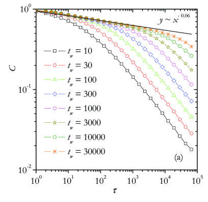
Considering this, the autocorrelation function (3) is expected to behave as Godreche1 ; Pleimling1

$$C(t,t_{w})={t_{w}}^{-b}f_{C}\left(\frac{t}{t_{w}}\right).$$ (10)

For $\tau\ll t_{w}$ ($\tau=t-t_{w}$), the critical scaling function $f_{C}(x)$ behaves as

$$f_{C}(x)\sim[x-1]^{-b}.$$ (11)

For $d$ dimensional spin glasses it has been foundOgielski1 ; Henkel1 that

$$b=\frac{d-2+\eta}{2z_{c}}.$$ (12)

Here $\eta$ is the static critical exponent associated to the pair correlation function. Then, for $\tau\ll t_{w}$ the autocorrelation function is

$$C(t,t_{w})\sim\tau^{-b}.$$ (13)

On the other hand, when $\tau\gg t_{w}$ we have:

$$f_{C}(x)\sim A_{C}x^{-\lambda_{C}/z_{c}},$$ (14)

where $A_{C}$ is a constant and $\lambda_{C}$ is known as the autocorrelation exponent. Henkel1

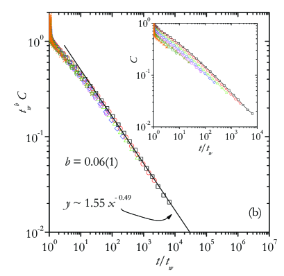
The Fig. 1(a) shows the behavior of the autocorrelation function $C(t,t_{w})$ vs $\tau$ for eight different waiting times $t_{w}$. For $\tau\ll t_{w}$ we can fit a power law behavior, $\tau^{-b}$, with exponent $b\approx 0.06$, as shown in the plot. For $\tau>t_{w}$ we observe that the correlation function shows aging since it depends strongly on the waiting time $t_{w}$. In the inset of Fig. 1 (b) we show the result of assuming “simple aging” by plotting $C$ as a function of the ratio $t/t_{w}$. We observe that the data does not show a good collapse in a single curve in this case. A good data collapse can be obtained if the “multiplicative aging” scaling form of Eq.(10) is assumed. In Fig. 1 (b), we show the plot of $t_{w}^{b}C$ vs. $t/t_{w}$, obtaining good scaling with $b=0.06(1)$. This value is in good agreement with Eq. (12): if we take from previous simulations of the 3D GG model the values $\eta=-0.47(2)$ Katzgraber1 and $z_{c}=4.5(1)$ Katzgraber2 we obtain $b=0.059(4)$. We now consider the case of $\tau\gg t_{w}$. In the Fig. 1 (b) we show that in this case the asymptotic behavior of $C$ has a power law form consistent with Eq.(14). We obtain $A_{C}=1.55(5)$ and $\lambda_{c}/z_{c}=0.49(2)$.

We now consider the autoresponse function. In this case the scaling equation is Godreche1

$$R(t,t_{w})={t_{w}}^{-1-a}f_{R}\left(\frac{t}{t_{w}}\right),$$ (15)

For $\tau\gg t_{w}$ is expected that

$$f_{R}(x)\sim A_{R}x^{-\lambda_{R}/z_{c}}$$

where $A_{R}$ is a constant amplitude. Then, if we consider Eq. (7), we obtain the thermoremanent reduced integrated response

$$\rho_{TRM}(t,t_{w})={t_{w}}^{-a}f_{\rho}\left(\frac{t}{t_{w}}\right),$$ (16)

where

$$f_{\rho}(x)\sim A_{\rho}x^{-\lambda_{R}/z_{c}},$$ (17)

and $A_{\rho}$ is a constant. For critical systems it is expected that $a=b$, and $\lambda_{C}=\lambda_{R}$.

Figure 2: (Color online) (a) Function $\rho_{TRM}$ vs $\tau$ for different waiting times and $h=0.05$. All symbols are the same as in Fig. 1 (a). (b) Data collapsing. Inset: Function $\rho_{TRM}$ vs $t/t_{w}$ for different waiting times and $h=0.05$.

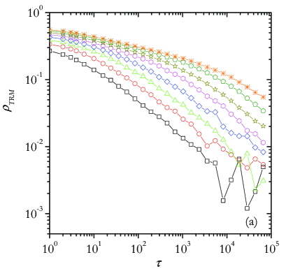
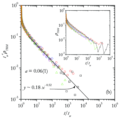
In Fig. 2 (a) we show the behavior of $\rho_{TRM}$ function vs $\tau$ for different waiting times and $h=0.05$, observing that the response function also shows aging. In the inset of Fig. 2 (b) we show $\rho_{TRM}$ vs $t/t_{w}$: no data collapse is observed. In Fig. 2 (b) we plot $t_{w}^{a}\rho_{TRM}$ vs $t/t_{w}$, obtaining good data collapse for $a=0.06(1)$. The asymptotic behavior observed for large temporal separations ($\tau\gg t_{w}$) can be fitted with a power law with $A_{\rho}=0.18(2)$ and $\lambda_{R}/z_{c}=0.52(2)$.

At thermodynamic equilibrium the fluctuation-dissipation theorem (FDT) is satisfied, and therefore it is possible to draw a simple expression to relate the correlation with the thermoremanent reduced integrated response

$$\rho_{TRM}(t-t_{w})=C(t-t_{w}).$$ (18)

Then, for a parametric plot of $\rho_{TRM}$ vs. $C$, we should obtain a straight line of slope $+1$ in equilibrium. On the other hand, for a nonequilibrium process the FDT is not fulfilled, and it has been proposed a generalized relation of the form

$$\rho_{TRM}(t,t_{w})=X(t,t_{w})C(t,t_{w}),$$ (19)

where $X(t,t_{w})$ is called the fluctuation-dissipation ratio (FDR). Cugliandolo For $1\ll t_{w}\ll t$ we can estimate the limit :

$$X_{\infty}=\lim_{t_{w}\rightarrow\infty}\lim_{t\rightarrow\infty}X(t,t_{w}).$$

For a critical quench, $X_{\infty}$ is expected to be universal in the sense that it does not depend neither on the initial conditions nor on the details of the dynamics. Godreche2

Figure 3: (Color online) FDT plot for different waiting times and $h=0.05$. All symbols are the same as in Fig. 1 (a).

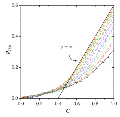
The Fig. 3 shows the $t$-parametric plot of $\rho_{TRM}(t,t_{w})$ vs $C(t,t_{w})$ for different waiting times $t_{w}$. In the quasi-equilibrium regime ($\tau\ll t_{w}$) the FDT holds and $X=1$. This is observed in Fig. 3 where for large $t_{w}$ the slope in the FDT plot tends to $1$. On the other hand, when $1\ll t_{w}\ll t$, we observe that $X<1$ and FDT is violated. From Eqs. (10), (14), (16), (17) and (19), it is possible to demonstrate that

$$X_{\infty}=A_{\rho}/A_{C}.$$

From the amplitudes $A_{C}$ and $A_{\rho}$ calculated previously we obtain $X_{\infty}=0.12(2)$.

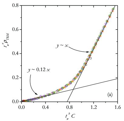
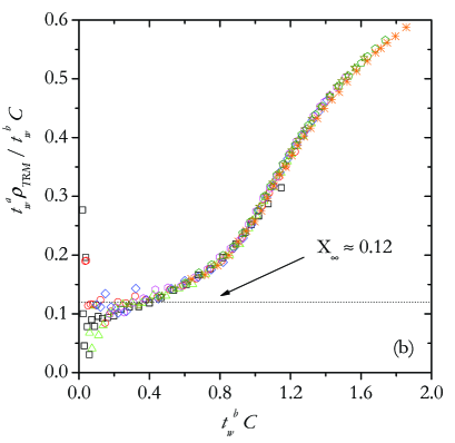
We can obtain $X_{\infty}$ numerically from the FDT plot of Figure 3 in two different ways. First, in Fig. 4 (a) we show a data collapse plotting $\rho_{TRM}(t,t_{w})t_{w}^{a}$ vs $C(t,t_{w})t_{w}^{b}$. The slope near the origin corresponds to the limit of FDR, obtaining $X_{\infty}=0.12(1)$. Second, in Fig. 4 (b) we plot the ratio ${t_{w}}^{a}\rho_{TRM}/{t_{w}}^{b}C$ vs ${t_{w}}^{b}C$ for all times $t$ and $t_{w}$. We see that the ordinate at the origin is compatible with $X_{\infty}\approx 0.12$.

Figure 4: (Color online) (a) Data collapsing for all curves in Fig. 3. (b) Plot of ratio ${t_{w}}^{a}\rho_{TRM}/{t_{w}}^{b}C$ vs ${t_{w}}^{b}C$. All symbols are the same as in Fig. 1 (a).

V DISCUSSION

We have therefore obtained the exponents that characterize the aging scaling of the 3D GG model at the critical temperature, obtaining $b=0.06(1)$, $\lambda_{C}/z_{c}=0.49(2)$, $a=0.06(1)$, $\lambda_{R}/z_{c}=0.52(2)$, and $X_{\infty}=0.12(1)$. A comparison with results in the corresponding model without disorder, i.e. the 3D XY model, shows that the exponents are very different, as expected. Abriet and Karevski,Abriet2 have found $a=b=1/2$, $\lambda_{C}/z=\lambda_{R}/z=1.34$, which shows that in the disorder-free case the “multiplicative” scaling of aging is stronger (i.e., much larger values of $a$ and $b$). Also a very different limit of the FDR, $X_{\infty}=0.43(4)$, was obtained, as expected since they should belong to different universality classes.

On the other hand, the critical aging of the GG turns out to be very similar to results found in the 3D ISG. Henkel1 ; Pleimling1 It has been found for a binary distribution in the exchange couplings: $a=0.060(4)$, $b=0.056(3)$, $\lambda_{C}/z=0.362(5)$, $\lambda_{R}/z=0.38(2)$ and $X_{\infty}=0.12(1)$; and for a Gaussian distribution in the exchange couplings: $a=0.044(1)$, $b=0.043(1)$, $\lambda_{C}/z=0.320(5)$, $\lambda_{R}/z=0.33(2)$ and $X_{\infty}=0.09(1)$. Henkel1 As we can see, the aging exponents are slightly smaller in the 3D ISG (meaning a weaker multiplicative aging), but the values of $X_{\infty}$ are comparable within the statistical error with the GG. It has been argued in Ref. Calabrese1, ; Godreche1, ; Godreche2, that $X_{\infty}$ is a novel universal quantity of non-equilibrium critical dynamics. It is interesting to observe that spin glass models like the ISG and GG have similar values of $X_{\infty}$. However, let us remind that most work on the equilibrium properties of the GG and the ISG show evidence that they are in different universality classes.Reger ; gingras ; moore ; Olson1 ; Katzgraber2

As discussed in the introduction, two types of behaviors are predicted for the vortex glass transition: either a finite temperature critical point as described by the GG, or a crossover temperature as found in the IFL. The work of Bokil and YoungBokil discards the first scenario. However, from the experimental point of view, the issue is not clearly resolved since several experiments show reasonably good scaling at a transition temperature.petrean Comparing our results with the behavior found by Bustingorry et al.Busting in the IFL, we believe that a study of the non-equilibrium dynamics of the vortex glass transition will be able to clearly distinguish between the two models. In simulations of the IFL , off-equilibrium correlation and response functions are found to scale as $B(t,t_{w})\sim t_{w}^{\alpha}\tilde{B}(t/t_{w})$, and also it is found that $\tilde{B}(x)\sim x^{\alpha}$ for $x\gg 1$.Busting The first thing to notice when comparing with critical aging in the GG is that, in the IFL, the corresponding multiplicative aging exponent $b$ and the autocorrelation exponent $\lambda_{C}/z$ coincide $b=\lambda_{C}/z=\alpha$ (and similarly for the response exponents, $a=\lambda_{R}/z=\alpha$). The second main difference is that the “multiplicative” aging in the IFL is very strong, $b_{\rm IFL}=\alpha\approx 0.25-0.35$ when compared with the GG at the critical point, $b_{\rm GG}\approx 0.06$. In the IFL the competition between the elasticity of each flux line and the randomness of the pinning potential leads to a very slow dynamics and strong aging with a large $\alpha$ exponent. Moreover, $\alpha$ depends with the disorder strength in the IFL, being larger for stronger disorder.

In this work we have analyzed the correlation and integrated response functions defined in Eqs.(3) and (9), since they are easy to compute numerically. In experiments in superconductors, correlation (response) functions of other observables like magnetization (magnetic susceptibility) and voltage (resistance) are, of course, more available. Aging scaling similar to Eqs.(10) and (16) will also be expected in these other physical quantities. For example, one possible way of observing experimentally the out-of-equilibrium dynamics of the vortex glass is monitoring the magnetic relaxation as done in Ref.papa, for granular samples. Another possibility is to perform electrical transport experiments near the transition temperature following a protocol similar to the one used by Ovadyahu and coworkers to study the electron glass regime in Anderson insulators. ovadyahu In either case, an analysis of the multiplicative aging exponent will clearly distinguish among the two different models ($b_{\rm IFL}\approx 0.25-0.35$ or $b_{\rm GG}\approx 0.06$).