Optimal Langevin modelling of out-of-equilibrium molecular dynamics simulations

Abstract

We introduce a scheme for deriving an optimally-parametrised Langevin dynamics of few collective variables from data generated in molecular dynamics simulations. The drift and the position-dependent diffusion profiles governing the Langevin dynamics are expressed as explicit averages over the input trajectories. The proposed strategy is applicable to cases when the input trajectories are generated by subjecting the system to a external time-dependent force (as opposed to canonically-equilibrated trajectories). Secondly, it provides an explicit control on the statistical uncertainty of the drift and diffusion profiles. These features lend to the possibility of designing the external force driving the system so to maximize the accuracy of the drift and diffusions profile throughout the phase space of interest. Quantitative criteria are also provided to assess a posteriori the satisfiability of the requisites for applying the method, namely the Markovian character of the stochastic dynamics of the collective variables.

With modern molecular dynamics approaches it is possible to follow the dynamical evolution of systems composed by a large number of particles. The resulting trajectory, obtained through numerical integration of the equations of motion, corresponds to a discrete trace in a phase space of very high dimensionality. In order to analyze this trajectory it is customary to monitor the time evolution of only a limited number of collective variables, also referred to as reaction coordinates, or order parameters. The latter are explicit functions of the microscopic degrees of freedom of the system for which they ought to provide a viable coarse-grained description. The system dynamics and equilibrium properties are then characterized in terms of these variables alone.

This dimensional reduction strategy, which has ubiquitous applications in physics and chemistry and biophysics (see e.g. refs. Garcia (1992); Kumar et al. (1992); Micheletti et al. (2003); Min et al. (2005a)), has its most-general formulation in the Zwanzig-Mori projection procedureZwanzig (1961). This scheme is of fundamental conceptual importance given its general formal applicability to systems whose evolution is governed by a Liouville operator. In such contexts it can be demonstrated that the time evolution of the collective variables is describable by a stochastic dynamics with a non-trivial memory kernel. Owing to the formidable difficulties posed by the a priori determination of the memory kernel, how to devise practical and general algorithms for carrying out the dimensional reduction remains an active area of research.

Several approaches have been developed over the years to perform dimensional reduction in specific contextsRisken (1989); Gullingsrud et al. (1999); Lange and Grubmüller (2006); Min et al. (2005b); Hummer (2005); Behrens et al. (2003); Kopelevich et al. (2005); Horenko et al. (2006); Lange and Grubmueller (2006); Kneller and Hinsen (2001). The validity of the overdamped Langevin dynamics is very commonly assumed a priori for describing the dynamical evolution of the reduced system. Consequently, the system free energy landscape and the diffusion coefficient profile can be expressed in terms of the Kramers-Moyal coefficients calculated a posteriori from extensive dynamical trajectories Risken (1989). An interesting illustration of this strategy is provided in ref. Kopelevich et al. (2005) where Kopelevich et al. estimate the Langevin drift and diffusion coefficients from short trajectories with different initial conditions. In other commonly-employed approaches the Langevin equation parameters are derived from a maximum likelihood principleGullingsrud et al. (1999); Hummer (2005); Horenko et al. (2006). Specifically, the free energy and diffusion coefficient profiles are chosen in such a way that the time evolution of the collective variables actually observed in the molecular dynamics trajectory has the highest realization probability. The latter is quantified by computing the Onsager-Machlup action along the trajectory, see the work of Gullingsrud et al. Gullingsrud et al. (1999). As shown by Hummer Hummer (2005), this scheme can also be generalized by allowing for a position-dependent diffusion coefficient. Another powerful related approach is the one of Horenko et al. Horenko et al. (2006) where the evolution of a system is assimilated to a diffusive process in a series of harmonic free energy wells. Transitions between the wells are described as discontinuous “jump” processes, with a suitable transition probability per unit time. The parameters of the model (the position and width of the harmonic wells, the diffusion coefficients in the wells and the jumping rates) are also derived a posteriori from a maximum likelihood approach.

Most available approaches have been formulated and designed to be applied to take as input equilibrated (canonical) trajectories. Recent advances in thermodynamic sampling techniques, however, stimulate the formulation of more general approaches applicable to systems subjected to external time-dependent biases. Large systems with a corrugated energy landscape would spontaneously evolve very slowly and the introduction of suitable external forces provides an effective means of driving the system through the reduced phase space. This is commonly exploited in several thermodynamic sampling techniques, such as steeringIzrailev et al. (1998), local-elevationHuber et al. (1994) adaptive force biasDarve and Pohorille (2001), flooding Grubmüller (1995), Wang-LandauWang and Landau (2001) and metadynamicsLaio and Parrinello (2002); Micheletti et al. (2004). To the best of our knowledge, the method of Gullingsrud et al. Gullingsrud et al. (1999) is the only available maximum-likelihood approach which is applicable to systems (whose diffusion coefficient is known a priori) subjected to externally-applied biases.

Building on the previous studies mentioned above, we here formulate and apply a novel maximum-likelihood scheme that allows to recover efficiently the equilibrium and dynamic properties of the reduced system even when subjected to an externally-applied time-dependent force. The variational approach addressed in this study complements the advantages of the strategies in refs. Hummer (2005) and Gullingsrud et al. (1999) as it allows recovering a posteriori a non-constant diffusion coefficient profile while accounting for externally-applied forces.

The method provides not only the drift and diffusion coefficients for the system (in one or more collective variables) but also an estimate of their statistical errors. For all these quantities we derive expressions that are straightforwardly calculated by averaging suitable observables along the dynamical trajectories. The possibility to control the error on the drift and diffusion terms of the reduced system opens the possibility to design the applied external bias so to achieve a pre-assigned profile of statistical uncertainties for the quantities of interest.

In the following we shall first derive the maximum-likelihood expressions for the drift and diffusion coefficient profiles and their errors. The advantages and range of applicability of the method are finally illustrated and discussed for a specific system, namely the problem of looping of a self-avoiding polymer chain in a crowded medium.

It should be remarked that the validity of the approach relies crucially on an appropriate choice of the collective variable whose dynamics, sampled at appropriate time intervals, must have a Markovian character. This requirement is not necessarily fulfilled by an arbitrarily chosen variable. Indeed, even if the trajectory of the system is generated by a Markovian process (e.g. molecular dynamics with Langevin thermostats), the dynamics of a single, projected variable cannot be expected to be Markovian tooZwanzig (1961). Though no simple a priori criteria can be adopted for a good choice of collective variables we discuss, in section II.4, how quantitative schemes can be introduces for verifying a posteriori if a given time series is reliably described by a Morkovian process and if the overal approach can consistently be applied.

I Optimal Langevin description of a stochastic dynamics process

We consider a system with several microscopic degrees of freedom and whose salient properties are described through a much smaller number of collective variables (CVs), $s_{i=1,...N}$, chosen a priori and defined in terms of the microscopic variables. The system is assumed to evolve in time under the combined action of two kind of forces: (i) the thermodynamic force, tending to establish the canonical equilibrium associated to a given temperature $T$, and (ii) a time-dependent external force acting on the collective variables. In the following we shall indicate with $\theta_{i}(t)$ the instantaneous external force conjugated to the $i$th collective variable. A prototype system, which will be discussed later, is constituted by a polymer chain where the fundamental degrees of freedom are the centers of its spherical monomers. A single collective variable will be used, namely the polymer end-to-end distance. The polymer dynamics is controlled by both the thermal buffeting of the surrounding solvent molecules and by an externally-controlled stretching force applied to the chain ends.

The evolution of the system is followed at the level of the collective variables through an equispaced time series $\mathcal{T}=\left\{s\left(0\right),s\left(dt\right),\dots,s\left(t\right),\dots\right\}$, where $s\left(t\right)$ denote the array of the instantaneous CV’s values, $s_{i=1,...,N}\left(t\right)$. The objective is to take the discrete trajectory $\mathcal{T}$ and the accompanying time series of the externally-applied forces, $\left\{\theta\left(0\right),\theta\left(dt\right),\dots,\theta\left(t\right),\dots\right\}$, as the sole inputs for deriving the best parametrization of the system properties within a Langevin description of the CV’s evolution. In particular, the aim is to recover the thermodynamic forces and diffusion matrices of the isolated system for a wide range of CV’s values by recording how the externally-driven system evolves.

The extraction of the optimal Langevin parametrization is carried out within a maximum likelihood approach, a framework profitably used in other previous approachesGullingsrud et al. (1999); Horenko et al. (2006); Hummer (2005). We start by assuming that for a suitable choice of the discretization time interval, $dt$, the CV’s evolution is describable as a Markovian process. The probability to observe a specific trajectory $\mathcal{T}$ is accordingly

$$P[\mathcal{T}]\propto{\prod_{t}}\pi\left(s(t),ds\left(t\right)\right)$$ (1)

where $ds_{i}\left(t\right)\equiv s_{i}\left(t+dt\right)-s_{i}\left(t\right)$ and $\pi\left(s(t),ds\left(t\right)\right)$ is the probability of the elementary step.

For non-externally-driven systems, described by a single collective variable, $s$, subject to an overdamped Langevin evolution with constant diffusion coefficient $D$ in a free energy landscape, $\mathcal{F}(s)$, the probability of the elementary step has a simple Gaussian form: $\pi\left(s(t),ds\right)\propto\frac{1}{\sqrt{D}}\exp{\left[-\frac{1}{4Ddt}\left(ds+\left(D\partial\mathcal{F}\left(s\right)\right)dt\right)^{2}\right]}$ Risken (1989). For simplicity of notation in the previous expression and in the following it is implied that the free energy $\mathcal{\ F}$ is expressed in units of the thermal energy, $\kappa_{B}\,T$. For the case of several collective variables and if the diffusion coefficients depends on the CV’s themselves, the previous expression generalizes toRisken (1989):

$$\pi\left(s,ds\right)\propto\frac{1}{\det D\left(s\left(t\right)\right)^{\frac{1}{2}}}\exp{\left[-\frac{1}{4dt}D_{ij}^{-1}(s\left(t\right))\chi_{i}\left(t\right)\chi_{j}\left(t\right)\right]}$$ (2)

where a summation of repeated indexes is implied and

$$\chi_{i}\left(t\right) = ds_{i}\left(t\right)+\left(D_{ij}\left(s\right)\partial_{j}\mathcal{F}\left(s\right)-\partial_{j}D_{ij}(s)\right)dt$$ (3)

$$= ds_{i}\left(t\right)-v_{i}\left(s\right)\,dt.$$

where $v_{i}(s)$ is the drift fieldRisken (1989). Without loss of generality, the diffusion matrix is assumed to be symmetric: $D_{ij}(s)=D_{ji}(s)$Risken (1989). Eq. (1), (2) and (3), for a given choice of $D\left(s\right)$ and $v\left(s\right),$ allow computing the probability of a trajectory $\mathcal{T}$. The stochastic differential equation leading to Eq. (2) and (3) is given by

$$ds_{i}\left(t\right)=v_{i}\left(s\left(t\right)\right)dt+\sqrt{2}\,\,D_{ij}^{1/2}(s\left(t\right))\,dW_{j}\left(t\right)$$ (4)

where $\{dW_{i}\left(t\right)\}$ is a $N-$dimensional Wiener process.

In the presence of the external force $\theta_{l}\left(t\right)$, Eq. (3) is modified as follows:

$$\chi_{i}\left(t\right) = ds_{i}\left(t\right)+\left(D_{ij}\left(s\right)\partial_{j}\mathcal{F}\left(s\right)\right.$$ (5)

$$\ \ \ \ \left.-D_{il}\left(s\left(t\right)\right)\theta_{l}\left(t\right)-\partial_{j}D_{ij}(s)\right)dt$$

$$= ds_{i}\left(t\right)-v_{i}\left(t\right)\,dt-D_{il}\left(s\left(t\right)\right)\theta_{l}\left(t\right)dt\ .$$

The extra term would contribute a term $-D_{ij}\left(s\right)\theta_{j}\left(t\right)dt$ in Eq. (4).

Eq. (1), supplemented by the relations of Eq. (2) and (3), coincides with the expression of the Onsager-Machlup actionRisken (1989), namely with the probability to observe the trajectory $\mathcal{T}$ given the known diffusion and drift terms governing its langevin evolution. In the present context , the probability $P[\mathcal{T}]$ of Eq. 1 can also be profitably interpreted from a complementary perspective. In fact, for a given trajectory, $P[\mathcal{T}]$ can be considered as a likelihood functional which characterizes the non-externally-driven system in terms of $v$ and $D$ . In this approach, extremizing Eq. (1) provides the unknown drift and diffusion terms ($v$ and $D$) yielding the highest possible probability for the given observed trajectory, $\mathcal{T}$.

Notice that, at variance with other approachesGullingsrud et al. (1999); Hummer (2005), the likelihood of the trajectory is here maximized with respect to the drift field $v_{i}(s)$ and not the free energy $F(s)$. An advantage of this alternative approach is that the solution can be expressed as an explicit average computed over the trajectory, at least in the one dimensional case (see Eq. (10)). The disadvantage is that, when two or more collective variables are used, the optimal $v$ and $D$ are not guaranteed to yield an equilibrium probability measureRisken (1989), but only to a stationary one. This condition should indeed be verified a posteriori and provides a further consistency criterion for the viability of the approach.

The cardinal variational equations for the drift and diffusion terms are $\frac{\delta\log P[\mathcal{T}]}{\delta v_{i}(s)}=0$ and $\frac{\delta\log P[\mathcal{T}]}{\delta D_{ij}(s)}=0$. After some algebra one obtains:

$$\frac{\delta\log P[\mathcal{T}]}{\delta v_{i}(s)}={\frac{D_{ij}^{-1}(s)}{2}}\sum_{t}\chi_{j}\left(t\right)\delta_{s-s\left(t\right)}$$ (7)

$$= {\frac{D_{ij}^{-1}}{2}}(s)\sum_{t}\delta_{s-s\left(t\right)}[ds_{j}-v_{j}dt-D_{ij}\theta_{l}dt]=0$$

$$\frac{\delta\log P[\mathcal{T}]}{\delta D_{ij}(s)}=\sum_{t}\left[-\frac{1}{2}D_{ij}^{-1}(s)+\right.$$

$$\frac{1}{4dt}D_{il}^{-1}\left(s\right)D_{jm}^{-1}(s)\chi_{l}\left(t\right)\chi_{m}\left(t\right)+\frac{1}{4}D_{il}^{-1}\left(s\right)\chi_{l}\left(t\right)\theta_{j}\left(t\right)$$

$$\left.+\frac{1}{4}D_{jl}^{-1}\left(s\right)\chi_{l}\left(t\right)\theta_{i}\left(t\right)\right]\delta_{s-s\left(t\right)}=0$$

where the condition $D_{ij}=D_{ji}$ has been enforced while taking the variation with respect to $D$. Introducing the notation $\left\langle a\right\rangle_{s}=\frac{\sum_{t}\delta_{s-s\left(t\right)}a\left(t\right)}{\sum_{t}\delta_{s-s\left(t\right)}}$, we obtain the following equations, that, in general, have to be solved self-consistently:

$$v_{i}\left(s\right) = \frac{1}{dt}\,\left\langle ds_{i}\right\rangle_{s}-D_{ij}\left(s\right)\left\langle\theta_{j}\right\rangle_{s}\ .$$ (8)

$$D_{ij}\left(s\right) = {\frac{\left\langle ds_{i}ds_{j}\right\rangle-\left\langle ds_{i}\rangle\langle ds_{j}\right\rangle}{2\,dt}}$$ (9)

$$+{\frac{D_{ip}(s)D_{kj}(s)}{2}}dt(\left\langle\theta_{p}\theta_{k}\right\rangle-\left\langle\theta_{p}\rangle\langle\theta_{k}\right\rangle)$$

Eqs. (8) and (9) make possible to estimate $D\left(s\right)$ and $v\left(s\right)$ also from trajectories obtained in the presence of time-dependent forces acting on the system. It is noteworthy that Eqs. (8) and (9) tie the optimal estimates of $v$ and $D$ to suitable averages made on the trajectory. On one hand this lends to a straightforward numerical implementation of the scheme. On the other, it highlights a key difference between the Eqs. (8) and (9) for driven systems and the Kramers-Moyal coefficients of first and second order which connect the Langevin and Fokker-Planck descriptions of the system evolution. At variance with the spirit of the averages in the above equations, in fact, the time-dependent Kramers-Moyal coefficients are defined as averages over the Wiener process at a given time and value of the CV’s. It is, however, clear that for a non-externally-driven system, where $\theta(t)=0$ at all times, the averages in Eqs. (8) and (9) coincide with those over independent realizations of the noise, and hence $v$ and $D$ match the time-independent Kramers-Moyal coefficients:

$$v_{i}\left(s\right) = \frac{1}{dt}\,\left\langle ds_{i}\right\rangle_{s}$$

$$D_{ij}\left(s\right) = {\frac{\left\langle ds_{i}ds_{j}\right\rangle-\left\langle ds_{i}\rangle\langle ds_{j}\right\rangle}{2\,dt}}\ .$$

In one dimension (namely for $N=1$) Eq. (9) can be explicitly solved also for $\theta\neq 0$. Since $D$ must be positive-defined, the second order Eq. (9) admits a single physically viable solution:

$$D\left(s\right)=\frac{-1+\sqrt{1+\left(\left\langle\theta^{2}\right\rangle_{s}-\left\langle\theta\right\rangle_{s}^{2}\right)\left(\left\langle ds^{2}\right\rangle_{s}-\left\langle ds\right\rangle_{s}^{2}\right)}}{dt\left(\left\langle\theta^{2}\right\rangle_{s}-\left\langle\theta\right\rangle_{s}^{2}\right)}$$ (10)

An important payoff of the maximum-likelihood approach is that it leads straightforwardly to estimating the uncertainty on the inferred values of $v_{i}^{\ast}$ and $D_{ij}^{\ast}$ (a star is used to denote the fact that these values maximize $P[\mathcal{T}]$), associated to the limited statistics inherent in any trajectory with finite duration. To do so we consider the expansion of $P[\mathcal{T}]$ around the maximum retaining terms up to quadratic order. Introducing an $N+N^{2}$ dimensional vector $y\left(s\right)=(\dots,v_{i}\left(s\right),\dots,D_{ij}\left(s\right),\dots)$, the error on $y_{i}$ at $s$, $\sigma^{2}\left(y_{i}\left(s\right)\right)$, can be estimated as the standard deviation of ${y_{i}(s)}$ from its best available estimate, ${y_{i}^{\ast}(s)}$. This is given by $\sigma^{2}\left(y_{i}\left(s\right)\right)=-\left(A^{-1}\right)_{ii}$ where

$$A_{ij}\left(s\right)=\left.{\frac{\delta^{2}\log\left(P[\mathcal{T}]\right)}{\delta y_{i}(s)\delta y_{j}(s)}}\right|_{y=y^{\ast}}$$ (11)

For $N=1$ we have

$$A\left(s\right)=-{\frac{N(s)dt}{2D}}\left(\begin{array}[]{cc}1&\langle\theta\rangle\\ \langle\theta\rangle&{\frac{1}{D\,dt}}[1+dtD\,\langle\theta^{2}\rangle]\end{array}\right)$$

with $N\left(s\right)=\sum_{t}\delta\left(s-s\left(t\right)\right)$. Thus, the uncertainties on $v$ and $D$ are given by

$$\sigma^{2}\left(v\left(s\right)\right) = \frac{2}{N(s)}\frac{D}{dt}\frac{1+dtD\,\langle\theta^{2}\rangle}{1+dtD(\langle\theta^{2}\rangle-\langle\theta\rangle^{2})}$$

$$\sigma^{2}\left(D\left(s\right)\right) = \frac{2}{N(s)}\frac{D^{2}}{1+dtD(\langle\theta^{2}\rangle-\langle\theta\rangle^{2})}$$ (12)

As intuitively expected, the quadratic error on $v$ and $D$ in $s$ are inversely proportional to $N\left(s\right)$, that is the number of times the trajectory visited $s$. For a trajectory generated by an ordinary dynamics on a system whose reduced free energy exhibits several minima saddle points etc., this error will be highly non-uniform. Even if transitions from the various basins are observed, the statistical accuracy on $v$ and $D$ in the transition region will degrade very rapidly with the barrier height. This limitations can be overcome with the aid of expression (12) and a preliminary rough knowledge of the free energy profile. In this case it is conceivable to design the application of the time-dependent external forces so to achieve an approximately uniform coverage of the phase space of interest. It should be remarked that Eq. (12) quantifies the statistical uncertainties on $v$ and $D$ and does not take into account possible systematic errors deriving from the non-Markovian nature of the process. These aspects will be discussed in more detail in Section II.E.

II Application: looping of a polymer chain

In the following we shall discuss the application of the above strategy to the problem of loop formation in a model polymer chain fluctuating in a solvent rich in crowding molecules. The polymer model considered here, follows the one introduced in Ref. Toan et al. (2006) to study how the polymer looping kinetics is affected by the crowding agents Marenduzzo et al. (2006). The novel question addressed here regards the possibility to describe the evolution of the polymer end-to-end distance, $s$, by means of a Langevin equation. It will be shown that, for a suitable choice of the time interval with which the original trajectory is sampled, a Langevin description for the evolution of $s$ is, in fact, possible. Interestingly, despite the simplicity of the system and its formulation, both the optimally-recovered drift and diffusion terms have a non-trivial dependence on $s$.

The model polymer consists of $n$ spherical beads of radius $R$ interacting via the following potential energy term:

$$V=\epsilon_{1}\sum_{i<j}e^{-a(d_{i,j}-2R)}-\epsilon_{2}\sum_{i}\ln[1-({\frac{d_{i,i+1}}{1.5\ R}})^{2}]$$ (13)

where the $i$ and $j$ denote the sequential indexing of the $n$ chain beads. The first term in expression (13) enforces the self-avoidance of the chain, while the second provides the attractive interaction between consecutive beads, thus enforcing the chain connectivity as in the FENE modelKremer and Grest (1990). The model parameters are exactly those introduced in Ref. Toan et al. (2006) to describe an eukariotic chromatin fiber, whose effective diameter and persistence length are both $\sim$ 25 nm Schiessel (2003). Specifically, $\epsilon_{1}$ and $\epsilon_{2}$ are respectively 1 and 70 units of thermal energy, $\kappa_{B}T$, $a=4$ nm^-1, and $R=12.5$nm is the bead radius. At the chosen temperature, $T=300$ K, the interplay of the two terms in (13) ensures that distance between consecutive beads fluctuates around the nominal value of 25 nm by only about 0.5 nm. The mass of the beads is calculated from the typical densities of biopolymers, $\rho=1.35$ g/cm³ Matthews (1968).

As anticipated, the motion of the chromatin fiber is assumed to occur in a medium crowded by other biomolecules (proteins, RNA etc.) which are simply modeled as monodispersed globular particles of radius $r=2.5$nm which altogether occupy 15% of the system volume. The crowding agents are not modelled explicitly but rather through the Asakura-Oosawa (AO) mean-field approach Asakura and Oosawa (1958). This approach exploits the smallness of the crowding agents compared to the chain beads, to introduce the effective self-attraction of the polymer, known as depletion interaction, induced by the hard-core repulsion with the crowding agents. This additional self-interaction is described by the following potential energy term:

$$V_{AO}=-\frac{\phi k_{B}T}{16r^{3}}\sum_{i<j}\left(2\tilde{d}_{ij}+3d_{ij}-\frac{3\Delta_{ij}^{2}}{4d_{ij}}\right)\ \tilde{d}_{ij}^{2}\ \Theta[\tilde{d}_{ij}]$$ (14)

where $\tilde{d}_{ij}=2r+d_{i,j}^{0}-d_{ij}$, $\Delta_{ij}=\left|R_{i}-R_{j}\right|$, and the step function $\Theta$ ensures that the AO depletion interaction vanishes at distances $>d^{0}+2r$. The dynamics of each bead (subjected to a Stokes-Einstein friction appropriate for molecular crowding Toan et al. (2006)) was followed within a under-damped Langevin schemeAllen and Tildesley (2001) with an integration time step of 1 ps, appropriate to resolve the decay of the correlation of the fastest-relaxing degrees of freedom of the system, the beads velocities. Part of the results presented below are obtained analyzing the end-to-end distance with a sampling time intervals of 200 ps or larger. The evolution of this quantity occurs over a time scale much larger than the relaxation time of the beads velocities and hence, for reasons of efficiency, was obtained through the over-damped Langevin schemeAllen and Tildesley (2001) with an integration time step of 15 ps. The equivalence of the under- and over-damped schemes was explicitly verified by comparing the estimates of the drift and diffusion coefficients obtained by processing runs covering 15 ms.

We first followed the evolution of the isolated system and used the recorded trajectory for the analysis presented in the previous section. We considered a single collective variable, namely the end-to-end distance, $s\left(r\right)=\left\|r_{N}-r_{1}\right\|$. As anticipated in the introduction, although the evolution of the original $n$-particle system is Markovian, the dynamics of $s\left(r\right)$ might not be necessarily so. This issue will be discussed in detail in Section II.4. We set the chain length, $n$, equal to 5; this made possible to collect extensive trajectories with an affordable computational effort and hence validate, at least in part, the variational Langevin description by comparing the predicted equilibrium properties against data obtained by straightforward histogram techniques.

II.1 Equilibrium properties of the optimal model

Figure 1: Evolution of the end-to-end distance in the absence (upper panel) and presence (lower panel) of an external force.

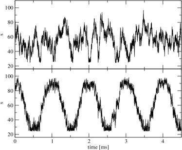
Starting from a random configuration of the polymer we have initially followed its underdamped Langevin dynamics (in the absence of any external force) over a time span of 180ms. As illustrated by the sample time series of $s$, shown in Fig. 1, upper panel, this time span is much larger than the typical looping/unlooping times of the chain, and hence is a sufficient guarantee of equilibration of the system properties. This trajectory was consequently used to estimate $v\left(s\right)$ and $D\left(s\right)$ and their errors from the averages in Eqs. (8), (9) and (12). In order to compute these averages it is necessary to choose the value for $dt$ entering in the Langevin equation. The correct $dt$ has to satisfy two conditions. First of all, $dt$ must be so large that the underlying process can be considered, at least approximately, as Markovian. At the same time, $dt$ has to be sufficiently small that the typical change of reaction coordinate over such time scale does not reflect in a significant variation of the free energy and diffusion coefficient.

This second condition can in principle be relaxed if the transition probability of the underlying Langevin process was known for an arbitrary $dt$ Horenko et al. (2006). Exact expressions for finite-time transition probabilities are however available for very special potentials, notably harmonic ones Horenko et al. (2006). In the present case, the free energy shape is not specified a priori, and hence it is necessary to use the approximation of Eq. (2), which is valid for small $dt$. Thus, the two conditions specified above may be potentially mutually exclusive.

For the simple polymer model described in this work it is possible to compute accurate equilibrium and kinetic quantities directly from extensive simulations, and choose a posteriori the value of $dt$ in order to obtain a Langevin model that reproduces them in as faithfully as possible. An alternative practical criterion for choosing this parameter without benchmarking the Langevin predictions against the exact results will be described in the following.

Figure 2: Free energy. Thick line: profile obtained from the the 180 ms trajectory. Other curves: free energy profiles reconstructed from the optimally determined $v(s)$ and $D(s)$, for various choices of $dt$. The free energies are from the histogram of $s$ as as $F\left(s\right)=-\frac{1}{\beta}\log N\left(s\right)=-\frac{1}{\beta}\log\int dt\delta\left(s-s\left(t\right)\right)$. The different curves are not distinguishable on the scale of the figure. Inset: zoom of the region of the first minimum, showing that small deviations from the true profile are observed for $dt>50ns$.

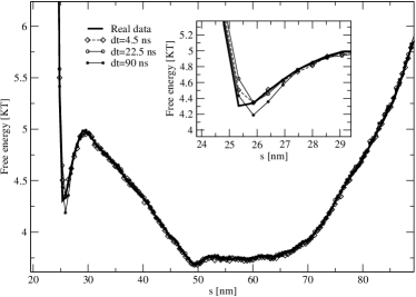
In Fig. 2, we compare the “true” canonical free energy of the system, $F(s)$, obtained through the histogram of the values of $s$ recorded in a long trajectory, with the one obtained computing $D$ and $v$ by equations (8), (9), and integrating numerically the stochastic differential equation formally given in eqn. (4). Specifically, the discrete-time evolution of $s$ implemented numerically was:

$$s(t+dt)=s(t)-v^{*}(s)dt_{l}+\sqrt{2D^{*}(s)dt_{l}}\cdot\eta(t)$$ (15)

where $\eta(t)$ is drawn from a Gaussian distribution with unit variance. In order to avoid systematic error deriving from a finite integration time, the time increment $dt_{l}$ is much smaller than $dt$. Qualitatively, the free energy profiles in Fig. 2 show two minima: one (denoted by $L$, for looped, in the following), for $s<27$, corresponding to a state in which the two ends of the polymer are in contact; the other (denoted by $U$, for unlooped), for $s>27$, corresponding to a state in which the two ends of the polymer are far. As we already remarked, $D$ and $v$ depend on the choice of the $dt$. The different curves are obtained solving the Langevin equation using $D$ and $v$ determined using with $dt=$4.5, 18 and 45 ns. All the choices lead to approximately the same profile. The profile starts degrading only for dt $>90ns$ (data not shown).

This provides an a posteriori demonstration that $D\left(s\right)$ and $v\left(s\right)$, if computed with an appropriate choice of $dt$, are consistent with the true equilibrium properties of the system.

II.2 Kinetic properties of the optimal model

Figure 3: Normalized histogram of the residence times in the L state, computed from the real dynamics and from the trajectories generated by the optimal model. The $L$ state corresponds to whenever $s$ is smaller than 26, and enters the $U$ state whenever $s$ is larger than 34.

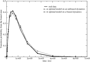
A complementary, stringent, test of the viability of the recovered $v^{\ast}$ and $D^{\ast}$ profiles can be performed by investigating kinetic-related properties of the system. The trajectory obtained from the Langevin model (15) was processed to calculate the average residence time in the bound state, namely the time $\tau_{1}$ required by the system entering in the $L$ state to escape from the well and entering in the $U$ state. The normalised distributions of $\tau_{1}$ obtained from the model Langevin equation (15) and from the original trajectory are shown in Fig. 3.

It can be seen that the two sets of distribution profiles are very consistent, thereby indicating the viability of the model Langevin description also for the kinetic system properties over time-scales much larger that $dt$.

II.3 Estimating the error

Figure 4: D(s) and v(s) evaluated with Eqs. (8) and (9) on an unbiased trajectory. Thick and thin lines are used for quantities obtained from trajectories of duration equal to 10ms and 0.5ms, respectively. The filled gray boxes represent the error bars calculated from Eqs. (12) for the 0.5 ms-long case.

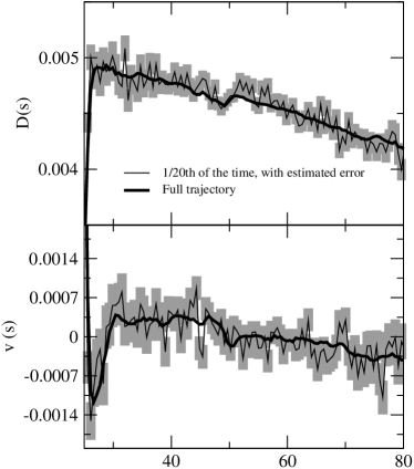
The validity of equation (12) for estimating the error has been tested by comparing $D\left(s\right)$ and $v\left(s\right)$ computed from trajectories of different length. The results are shown in Fig. 4. The thick line represent $D\left(s\right)$ and $v\left(s\right)$ computed using all the 180 ms of the trajectory. As we anticipated, even if the chosen collective variable is very simple, $D\left(s\right)$ shows significant variations as a function of $s$. The thin black line corresponds to the two quantities evaluated using a much shorter trajectory of 9 ms. The solid gray blocks are the estimated errors as given by Eqs. (12). The thin black lines falls well within the estimated error of the 180 ms result, showing that Eqs. (12) provide viable estimates for the statistical uncertainties.

II.4 Optimal model of the non-externally-driven system from an out-of-equilibrium trajectory

A major advantage of the approach presented here is that it can be applied also on trajectories generated under the action of an external time-dependent forces. To illustrate this point we now consider a trajectory of the system under the action of an external force of the form

$$\theta\left(t\right)=-\frac{d}{ds}\left[\frac{1}{2}k\left(s-s_{rest}\left(t\right)\right)^{2}\right]$$ (16)

If this force is applied, the system is biased towards following $s_{rest}\left(t\right)$.

Figure 5: Free energy profiles. Thick line: profile obtained from the histogram of the trajectory of the non-externally-driven system. Dashed line: free energy profile obtained from the optimal Langevin description applied to data recorded in the presence of the harmonic time-dependent external force. The continuous line provides, for comparison the “free-energy” profile obtained directly from the histogram of $s$ recorded in the run subject to the external force.

Although the externally applied force can be chosen a priori so to optimize the statistical uncertainty on the $D$ and $v$ profiles we shall consider the very simple case of an harmonic force derived from a harmonic restraining potential whose center is scillating between $s_{min}$ and $s_{max}$ with a period $T=1ms$:

$$s_{rest}\left(t\right)=s_{min}+\frac{1}{2}\left(s_{max}-s_{min}\right)\left(\cos\left(2\pi\frac{t}{T}\right)-1\right)$$ (17)

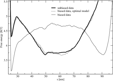
The values $s_{min}$ and $s_{max}$ are set equal to 21 and 104 nm, which hence cover a range of the original parameter space wide enough to encompass both minima of the free energy. A sample trajectory obtained under the action of this bias is shown in Fig. 1, lower panel. As visible, the added external force influences heavily the evolution of the system which, in fact, exhibits a noisy harmonic modulation. The external bias is so strong that a direct use of the the recorded $s$ trajectory to compute the system free energy from the usual histogramming procedure would lead to a completely wrong free energy profile (shown with a thin continuous line in Fig. 5). By contrast, the use of the optimal Langevin scheme derived above is very effective in subtracting the effect of the bias and yield a free energy profile that is entirely compatible with the true one. Notice that the bias subtraction does not exploit the knowledge of the instantaneous values of the external force, but relies merely on the knowledge of the time-averaged of the bias as a function of the collective variable.

II.5 Validity of the Markovian approximation and optimal choice of dt

As already mentioned, the choice of the time lag at which the data are recorded, $dt$, is essential for the viability and consistency of the proposed method, particularly regarding the Markovian character of the chosen collective variable. If $dt$ is too small, Eq. (4) is not adequate for describing the evolution of $s$, as the noise term (reflecting the influence of the “integrated” degrees of freedom) would have a sizable autocorrelation time. On the other hand, if the time lag is too large, there would be prominent variations of the free energy and diffusion coefficient evaluated for two “consecutive” positions, $s(t)$ and $s(t+dt)$. This would invalidate the assumption, see Eq. (15), that the force acting at time $t$ depends only on the instantaneous position, $s(t)$.

If the recovered diffusion coefficient is constant in parameter space and the underlying free-energy profile is harmonic, the Markovian character of the collective variable can be established by verifying the exponential decay of its autocorrelation function. More sophisticated procedures must be followed to compute the memory kernel when the drift and diffusion terms do not have a structure as simple as the one mentioned aboveKneller and Hinsen (2001); Lange and Grubmüller (2006). Here we show a series of simple quantitative tests that can be used to assess the Markovian character of the collective variable on the time-scale defined by the sampling interval $dt$. These tests can be easily used to find an optimal value of $dt$.

To this purpose we solve Eq. (4) with respect to the noise $dW_{j}\left(t\right):$

$$dW_{j}\left(t\right)=\frac{1}{\sqrt{2}}D_{ij}^{-1/2}\left(ds_{i}\left(t\right)-v_{i}\left(s\left(t\right)\right)dt\,\right)\ .$$ (18)

Using the estimates $v\left(s\right)$ and $D\left(s\right)$ given by Eqs. (8) and (9), one can evaluate $dW_{j}\left(t\right)$ along the trajectory $\left\{\dots,s\left(t\right),s\left(t+dt\right),\dots\right\}.$ It is readily seen that $dW_{j}\left(t\right)$ from Eq. (18) satisfies:

$$\left\langle dW_{i}\left(t\right)\right\rangle = 0$$

$$\left\langle dW_{i}\left(t\right)dW_{j}\left(t\right)\right\rangle = dt\delta_{ij}\ .$$

Yet, the internal consistency of the procedure requires that $dW_{j}\left(t\right)$ is uncorrelated at different times and that its probability distribution is Gaussian. These two properties are not enforced in the optimization procedure, and they can hence be used to validate, a posteriori its applicability.

Figure 6: Upper panel: Time correlation function $C_{dt}\left(\tau\right)=\frac{1}{dt}\left\langle dW\left(t\right)dW\left(t+\tau\right)\right\rangle$ as a function of $\tau/dt$ for different choices of $dt$. Lower panel: Probability distibution of $dW/\sqrt{dt}$ for different choices of the time lag $dt$. $dW$ is computed from Eq. (18) and the average is restricted to values of $t$ in which $27.5<s(t)<30.5$ (approximately the region of the barrier). Inset: normalized kurtosis, $\kappa\equiv(<dW^{4}>-3<dW^{2}>^{2})/dt^{2}=<dW^{4}>/dt^{2}-3$, as a function of the time lag $dt$.

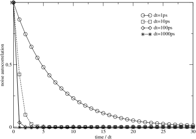
As a first step in the validation we calculate the autocorrelation function of the noise for given values of the time lag $dt$, $C_{dt}\left(\tau\right)=\frac{1}{dt}\left\langle dW\left(t\right)dW\left(t+\tau\right)\right\rangle$. The averages were calculated from a single underdamped Langevin evolution of the system and the sampling time-lag, $dt$, ranged between 0.001 and 2000 ns. The resulting autocorrelations as a function of $\tau/dt$ are shown in Fig. 6, upper panel. The trends should be compared with the step character of a memoryless noise: $C_{dt}\left(0\right)=1$ and $C_{dt}\left(\tau\right)=0$ for all $\tau\neq 0$. This limiting behaviour is well-approximated for large $dt$, as the autocorrelation drops almost immediately to zero ($C_{dt}\left(dt\right)\simeq 0.01$ for $dt=1$ ns). A slow decay is, instead observed for smaller $dt$’s, indicating that the underlying stochastic process derives from a correlated noise.

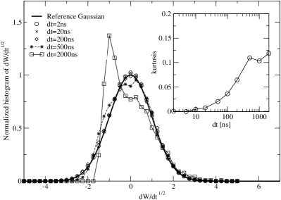
By inspecting suitable properties of the noise $dW_{j}\left(t\right)$ of Eq. (18) it is further possible to highlight the limitations of excessively-large values of $dt$. A valuable indicator is provided by the Gaussian character of the distribution of the instantaneous noise amplitudes$\frac{dW\left(t\right)}{\sqrt{dt}}$. The histograms in Fig. 6, lower panel, indicate noticeable deviations from Gaussianity for $dt$ larger than 500 ns. Also the normalized kurtosis (see Fig. 6, lower panel, inset) becomes significantly different from zero for $dt>$ 100 ns.

It emerges that $dt$ must be chosen so to satisfy simultaneously the criteria for the memoryless character of the noise and the Gaussianity of its probability distribution. For the specific system considered here, it can be verified that using $dt$ between 1 and 100 ns provides a viable and consisent Langevin description of the system. In fact, in these conditions, the autocorrelation function of the noise has the correct form and, at the same time, the probability distribution of $dW$ is very close to a Gaussian.

III Conclusions

We have presented an optimal scheme for describing a posteriori the dynamics of a given system through the Langevin evolution of few collective variables. The scheme lends to a straightforward numerical implementation. It allows one to extract not only the drift profile but also the diffusion coefficient which may both depend on the collective variables. The proposed methodology allows to control the statistical uncertainty affecting the calculated drift and diffusion profiles. Secondly, the drift and diffusion terms of the non-externally-driven system can be recovered from trajectories recorded in the presence of an externally-applied force. This second aspect appears particularly important as the external time-dependent force can be designed to optimize, for a given duration of the system evolution, the exploration of the phase space and control the statistical uncertainty on the parameters of the Langevin equation. The viability of the scheme was illustrated by applying it to the looping kinetics of a model polymer system. As several other approaches, the proposed one can be applied to systems describable by an overdamped Langevin dynamics. We plan to explore the feasibility of extending the present framework to the case of CV evolving under the action of non-trivial memory kernels. This would be a particularly important avenue for characterizing the salient dynamical features of biomolecules which is presently attracting considerable attention due to the large range of time scales that these molecules exhibit in their internal dynamics Kneller (2000); Hinsen et al. (2000); Kneller and Hinsen (2004); Min et al. (2005a); Pontiggia et al. (2007); Henzler-Wildman et al. (2007); Calandrini et al. (2008).

Acknowledgements We thank M. Parrinello for valuable discussions. We acknowledge financial support from the Italian Ministry for Education (FIRB 2003, grant RBNE03B8KK and PRIN, grant 2006025255) and from Regione Friuli Venezia Giulia (Biocheck, grant 200501977001).

References

- Garcia (1992) A. Garcia, Phys. Rev. Lett. 68, 2696 (1992).
- Kumar et al. (1992) A. Kumar, D. Bouzida, R. Swendsen, P. Kollman, and J. Rosenberg, J. Comp. Chem. 13, 1011 (1992).
- Micheletti et al. (2003) C. Micheletti, V. D. Filippis, A. Maritan, and F. Seno, Proteins 53, 720 (2003).
- Min et al. (2005a) W. Min, B. English, G. Luo, B. Cherayil, S. Kuo, and X. Xie, Acc. Chem. Res. 38, 923 (2005a).
- Zwanzig (1961) R. Zwanzig, Phys. Rev. 124, 983 (1961).
- Risken (1989) H. Risken, The Fokker-Planck Equation (Springer-Verlag, 1989).
- Gullingsrud et al. (1999) J. Gullingsrud, R. Braun, and K. Schulten, J. Comp. Phys. 151, 190 (1999).
- Lange and Grubmüller (2006) O. Lange and H. Grubmüller, J. Chem. Phys. 124, 214903 (2006).
- Min et al. (2005b) W. Min, G. Luo, B. Cherayil, S. Kou, and X. S. Xie, Phys. Rev. Lett. 94, 198302 (2005b).
- Hummer (2005) G. Hummer, New J. Phys. 7, 34 (2005).
- Behrens et al. (2003) S. Behrens, J. Plewa, and D. Grier, Eur. Phys. J. E 10, 115 (2003).
- Kopelevich et al. (2005) D. Kopelevich, A. Panagiotopoulos, and I. Kevrekidis, J. Chem. Phys. 122, 044908 (2005).
- Horenko et al. (2006) I. Horenko, E. Dittmer, A. Fischer, and C. Schütte, Mult. Mod. Sim. 5, 802 (2006).
- Lange and Grubmueller (2006) O. Lange and H. Grubmueller, J. Phys. Chem. B 110, 22842 (2006).
- Kneller and Hinsen (2001) G. Kneller and K. Hinsen, J. Chem. Phys. 115, 11097 (2001).
- Izrailev et al. (1998) S. Izrailev, S. Stepaniants, B. Isralewitz, D. Kosztin, H. Lu, F. Molnar, W. Wriggers, and K. Schulten, Steered molecular dynamics, in Computational Molecular Dynamics: Challenges, Methods, Ideas, vol. 4 (P. Deu hard, J. Hermans, B. Leimkuhler, A. E. Mark, S. Reich, and R. D. Skeel, Lecture Notes in Computational Science and Engineering, Springer-Verlag, Berlin, 1998).
- Huber et al. (1994) T. Huber, A. Torda, and W. van Gunsteren, J. Comput. Aided Mol. Des. 8, 695 (1994).
- Darve and Pohorille (2001) E. Darve and A. Pohorille, J. Chem. Phys. 115, 9169 (2001).
- Grubmüller (1995) H. Grubmüller, Phys. Rev. E 52, 2893 (1995).
- Wang and Landau (2001) F. Wang and D. Landau, Phys. Rev. Lett. 86, 2050 (2001).
- Laio and Parrinello (2002) A. Laio and M. Parrinello, Proc. Natl. Acad. Sci. USA 99, 12562 (2002).
- Micheletti et al. (2004) C. Micheletti, A. Laio, and M. Parrinello, Phys. Rev. Lett. 92, 170601 (2004).
- Toan et al. (2006) N. Toan, D. Marenduzzo, P. Cook, and C. Micheletti, Phys. Rev. Lett. 97, 178302 (2006).
- Marenduzzo et al. (2006) D. Marenduzzo, C. Micheletti, and P. Cook, Biophys. J. 90, 3712 (2006).
- Kremer and Grest (1990) K. Kremer and G. Grest, J. Chem. Phys. 92, 5057 (1990).
- Schiessel (2003) H. Schiessel, J. Phys.- Cond. Matt. 15, R699 (2003).
- Matthews (1968) B. Matthews, J. Mol. Biol. 33, 491 (1968).
- Asakura and Oosawa (1958) A. Asakura and F. Oosawa, J. Polym. Sci. 33, 183 (1958).
- Allen and Tildesley (2001) M. Allen and D. Tildesley, Computer Simulation of Liquids (Clarendon Press, Oxford, 2001).
- Kneller (2000) G. Kneller, Chemical Physics 261, 1 (2000).
- Hinsen et al. (2000) K. Hinsen, A.-J. Petrescu, S. Dellerue, M.-C. Bellissent-Funel, and G. Kneller, Chem. Phys. 261, 25 (2000).
- Kneller and Hinsen (2004) G. Kneller and K. Hinsen, J. Chem. Phys. 121, 10278 (2004).
- Pontiggia et al. (2007) F. Pontiggia, G. Colombo, C. Micheletti, and H. Orland, Phys. Rev. Lett. 98, art. no 048102 (2007).
- Henzler-Wildman et al. (2007) K. Henzler-Wildman, M. Lei, V. Thai, S. Kerns, M. Karplus, and D. Kern, Nature 450, 913 (2007).
- Calandrini et al. (2008) V. Calandrini, D. Abergel, and G. Kneller, J. Chem. Phys. 128, art. no. 145102 (2008).