On the probability distribution of stock returns in the Mike-Farmer model
Abstract
Recently, Mike and Farmer have constructed a very powerful and realistic behavioral model to mimick the dynamic process of stock price formation based on the empirical regularities of order placement and cancelation in a purely order-driven market, which can successfully reproduce the whole distribution of returns, not only the well-known power-law tails, together with several other important stylized facts. There are three key ingredients in the Mike-Farmer (MF) model: the long memory of order signs characterized by the Hurst index , the distribution of relative order prices in reference to the same best price described by a Student distribution (or Tsallis’ -Gaussian), and the dynamics of order cancelation. They showed that different values of the Hurst index and the freedom degree of the Student distribution can always produce power-law tails in the return distribution with different tail exponent . In this paper, we study the origin of the power-law tails of the return distribution in the MF model, based on extensive simulations with different combinations of the left part for and the right part for of . We find that power-law tails appear only when has a power-law tail, no matter has a power-law tail or not. In addition, we find that the distributions of returns in the MF model at different timescales can be well modeled by the Student distributions, whose tail exponents are close to the well-known cubic law and increase with the timescale.
keywords:
Econophysics; Mike-Farmer model; Power-law tail; -Gaussian; Order-driven market,
1 Introduction
Many stylized facts have been unveiled in different stock markets Mantegna-Stanley-2000 , Cont-2001-QF , Zhou-2007 . Understanding the underlying regularities causing stylized facts are crucial in stock market modeling. Three different families of market models exist aiming at reproducing the main stylized facts. The first family is the dynamic models, such as the multifractal model of asset returns Mandelbrot-Fisher-Calvet-1997 , which was later extended in several publications Calvet-Fisher-2001-JEm , Lux-2003 , Lux-2004 , Eisler-Kertesz-2004-PA , and the multifractal random walks Bacry-Delour-Muzy-2001-PA , Bacry-Delour-Muzy-2001-PRE , Pochart-Bouchaud-2002-QF . The second family is the agent-based models (or multi-agent models), in which agents buy or sell shares according to some rules and the price variations are determined by the imbalance of demand and supply. There are different types of agent-based models, such as percolation models Cont-Bouchaud-2000-MeD , Stauffer-1998-AP , Stauffer-Penna-1998-PA , Eguiluz-Zimmermann-2000-PRL , DHulst-Rodgers-2000-IJTAF , Xie-Wang-Quan-Yang-Hui-2002-PRE , Ising models Foellmer-1974-JMe , Chowdhury-Stauffer-1999-EPJB , Iori-1999-IJMPC , Kaizoji-2000-PA , Bornholdt-2001-IJMPC , Zhou-Sornette-2007-EPJB , minority games Arthur-1994-AER , Challet-Zhang-1997-PA , Challet-Marsili-Zhang-2000-PA , Jefferies-Hart-Hui-Johnson-2001-EPJB , Challet-Marsili-Zhang-2001-QF , Challet-Marsili-Zhang-2001a-PA , Challet-Marsili-Zhang-2001b-PA , Challet-Marsili-Zhang-2005 , and others Lux-Marchesi-1999-Nature . The minority games are among the most important agent-based models and thus many variants have been proposed. The third family is the order-driven models, where researchers attempt to simulate the dynamics of order books. The price in order-driven models changes based on the continuous double auction (CDA) mechanism Maslov-2000-PA , Daniels-Farmer-Gillemot-Iori-Smith-2003-PRL , Farmer-Patelli-Zovko-2005-PNAS . A nice review of order-driven models was recently given by Slanina Slanina-2008-EPJB . We can think of the agent-based models and the order-driven models as microscopic models for quote-driven markets and order-driven markets, respectively.
Recently, Mike and Farmer have constructed a very powerful and realistic behavioral model to mimick the dynamic process of stock price formation Mike-Farmer-2008-JEDC , which belongs to the third family. We call it Mike-Farmer model, or MF model for short. It seems undoubtable to us that the MF model is a milestone in the modeling of order-driven markets, which will prove to introduce an important improvement in asset derivative pricing and risk management. Having said this, we stress that the MF model is still very simple as mentioned already by Mike and Farmer Mike-Farmer-2008-JEDC and there are still a lot of open problems to be addressed. Indeed, the MF model provides a nice platform to unravel the origin of stylized facts of stocks in order-driven markets. The essential advantage of the MF model is that it is constructed based on the empirical regularities of order placement and cancelation in a purely order-driven market, which can successfully reproduce the whole distribution of returns, not only the well-known power-law tails, together with several other important stylized facts. There are three key ingredients in the MF model: the long memory of order signs characterized by the Hurst index , the distribution of relative order prices in reference to the same best price described by a Student distribution, and the dynamics of order cancelation.
Through extensive simulations, Mike and Farmer found that different values of the Hurst index and the freedom degree of the Student distribution can always produce power-law tails in the return distribution with different tail exponent . Specifically, they found that increases almost linearly with for fixed and decreases approximately linearly with for fixed . Our simulations of the MF model with different values of (ranging from 0.9 to 1.9 with a step of 0.1) and (ranging from 0.1 to 0.9 with a step of 0.1) confirm this finding. Speaking differently we have simulated versions of the MF model. For each version, four million simulation steps are conducted after removing the initial transient data and we obtain about one million data points of trade-by-trade returns. We find that the dependence of upon and can be modeled using the following formula:
| (1) |
These observations can be explained as follows. With the increase of , the memory of order signs becomes stronger and more orders of the same direction (buy or sell) are placed successively. This results in more large price fluctuations and the decay of becomes slower. Hence the tail exponent decreases. On the other hand, if is small, more passive orders with are placed deep inside the order book and the standing volumes close to the best ask or bid price are relatively small. Speaking differently, the depth of the order book is low and the liquidity is low. Also, there are more aggressive orders with placed resulting in more market orders. Both effects lead to more large price fluctuations and slower decay of the return distribution.
Although both the strength of the long memory of order signs and the tail exponent of relative order prices have significant influence on the distribution of returns, it is unclear what causes the power-law tails in the MF model. In this paper, we will address this question based on extensive simulations with different combinations of the left part for and the right part for of . We find that power-law tails appear only when has a power-law tail, no matter has a power-law tail or not. Moreover, we find that the return distributions in the MF model at different timescales can be well modeled by the Student (or Tsallis’ -Gaussian) distributions, whose tail exponents are close to the well-known cubic law and increase with the timescale.
2 Description of the Mike-Farmer model
In purely order-driven markets, the main trading mechanism is the continuous double auction. Passive traders are patient and place effective limit orders that are stored in the order book waiting for execution, while aggressive traders are inpatient and submit effective market orders that are executed immediately. Consider a limit order placed at event time whose logarithmic price is . Denote and the logarithms of best ask and bid prices right before . A buy limit order with or a sell limit order with is classified as an effective market order. Speaking differently, orders with the relative prices less than the preceding spreads are effective limit orders, while orders with are effective market orders111The relative price is defined as for buy orders and for sell orders.. Orders waiting on the limit order book are either satisfied by future effective market orders or canceled. Therefore, the continuous double auction can be simulated if one knows the regularities governing the dynamic processes of order placement and cancelation. Most order-driven models also follow this line. However, to the best of our knowledge, the MF model is the only one that uses empirical regularities of order placement and cancelation extracted from real stock data. This is the reason why the MF model can reproduce the cubic law of return distribution without tuning any model parameters. Actually, the MF model does not introduce any artificial tunable model parameters at all. All parameters in the MF model are determined empirically and have clear financial meanings. The regularities of order placement and cancelation may be different for different stock markets. The MF model can be easily modified for other markets.
When placing an order, the trader needs to determine its sign (“” for buys and “” for sells), size and price (or the relative price ). In the MF model, all orders are assumed to have identical size. The signs of successive orders have strong memory, which can be characterized by a rather large Hurst index close to 0.8 or even larger Lillo-Farmer-2004-SNDE , Mike-Farmer-2008-JEDC . This finding is conclusive without any controversy. In contrast, the distribution of relative prices seems different in different markets. Zovko and Farmer studied the unconditional distribution of relative limit prices defined as the distance from the same best prices for orders placed inside the limit-order book Zovko-Farmer-2002-QF . They merged the data from 50 stocks traded on the London Stock Exchange (August 1, 1998 to April 31, 2000) and found that the distribution decays roughly as a power law with the tail exponent for both buy and sell orders. Bouchaud et al. analyzed the order books of three liquid stocks on the Paris Bourse (February 2001) and found that the relative price of new orders placed inside the book follows a power-law distribution with the tail exponent Bouchaud-Mezard-Potters-2002-QF . Potters and Bouchaud investigated the relative limit price distributions for inside-the-book orders of three Nasdaq stocks (June 1 to July 15, 2002) and found that the distributions exhibit power-law tails with an exponent Potters-Bouchaud-2003-PA . Maskawa analyzed 13 rebuild order books of Stock Exchange Electronic Trading Service from July to December in 2004 on the London Stock Exchange and found that the limit prices for all orders inside the book are broadly distributed with a power-law tail whose exponent is Maskawa-2007-PA , which is consistent with the results of Zovko and Farmer Zovko-Farmer-2002-QF . He also presented the distribution in the negative part for more aggressive order outside the book and found that the negative part decays much faster than the positive part. Mike and Farmer focused on the stock named AZN and tested on 24 other stocks listed on the London Stock Exchange (LSE) Mike-Farmer-2008-JEDC . They found that the distribution of relative logarithmic prices can be fitted by a Student distribution with degrees of freedom and the distribution is independent of bid-ask spread at least over a restricted range for both buy and sell orders. Gu, Chen and Zhou analyzed 23 Chinese stocks traded on the Shenzhen Stock Exchange (SZSE) and found that the distribution of relative prices is asymmetric Gu-Chen-Zhou-2008b-PA . They showed that the distribution has power laws with the exponents greater than 1 and lower than 2.
There are also efforts to seek for factors influencing order placement. Using 15 stocks on the Swiss Stock Exchange, Ranaldo found that both bid-ask spread and volatility negatively relate to order aggressiveness Ranaldo-2004-JFinM . Lillo analyzed the origin of power-law distribution of limit order prices considering the order placement as an utility maximization problem considering three factors: time horizon, utility function and volatility Lillo-2007-EPJB . He found that the heterogeneity in time horizon is the proximate cause of the asymptotic power-law distribution, while heterogeneity in volatility is hardly connected with the origin of power-law distribution. Mike and Farmer found that the distribution of LSE stocks is independent of the bid-ask spread Mike-Farmer-2008-JEDC , which was confirmed by Gu, Chen and Zhou using SZSE stocks Gu-Chen-Zhou-2008b-PA .
In a zero intelligence model Daniels-Farmer-Gillemot-Iori-Smith-2003-PRL , Farmer-Patelli-Zovko-2005-PNAS , order cancelation is assumed to be a Poisson process. Alternatively, Mike and Farmer found that the conditional probability of canceling an order at time is influenced by at least three factors Mike-Farmer-2008-JEDC : the ratio of current relative price of an order to its original relative price when it is placed, the number of orders in the order book, and the order book imbalance that is defined as the ratio of the number of buy (or sell) orders to . By assuming that , and are independent, the conditional probability of cancelation per order has the following form:
| (2) |
where the parameters and are determined empirically using real data of individual stocks Mike-Farmer-2008-JEDC .
Now we can describe the MF model as follows. We stress that the sizes of orders are set to unity. In each round of the simulation, we simulate steps and the first 2000 data points are discarded from the ensuing analysis. We repeat this process 20 times, which results in four million orders and about one million transactions. In each round, we generate two arrays of the relative prices and the order signs . The sign array of the orders is generated from a fractional Brownian motion with Hurst index and the relative price is taken from a Student distribution with scale and degrees of freedom. At each simulation step or event time , an order is generated, which is characterized by and . When , the order is executed and a buy limit order (if ) or a sell limit order (if ) at the best bid or ask price is removed from the order book. When , the order is stored in the order book at the price level , where is the tick size, is the largest integer smaller than , and for buy orders or for sell orders. We then calculate the values of for all orders waiting in the order book. A random number is drawn from a uniform distribution defined on the interval . All orders with are canceled from the order book. The returns between successive trades are used in this work. We note that the results presented in Mike-Farmer-2008-JEDC are successfully reproduced in our simulations.
3 The origin of power-law tail of returns
3.1 Methodology
Mike and Farmer have shown that the power-law tails in the return distribution become heavier if the long memory in the order signs is stronger Mike-Farmer-2008-JEDC . We notice that the power-law tails do not vanish even when . In other words, long memory in the order signs cannot explain the emergence of power-law tails of returns. Therefore, we turn to investigate the influence of on . According to the setting of the MF model, the shape of for does not impact the shape of , since those orders are effective market orders that always remove one unit of shares from the opposite side of the order book, despite of the true prices of the incoming effective market orders. We thus speculate that the right part of , denoted as , has much weaker influence than the left part . In our simulations, the tick size is and three model parameters are fixed according to Mike-Farmer-2008-JEDC : , , and .
In order to unveil the effect of the two parts of on the tail behavior of , we adopt different formulae for . In general, we can write the following
| (3) |
Obviously, when , we require that
| (4) |
In the MF model, . In this section, we will use different functional forms for and .
The first class is the Student density Blattberg-Gonedes-1974-JB or Tsallis’ -Gaussian Tsallis-Anteneodo-Borland-Osorio-2003-PA , whose density is
| (5) |
where is the degrees of freedom parameter (or tail exponent), is the scale parameter, and is the Beta function, that is, with being the gamma function. The second class is the Laplace distribution or double exponential distribution, whose density is
| (6) |
and the third class is the normal distribution, whose density is
| (7) |
According to the symmetry of the distribution of in the MF model Mike-Farmer-2008-JEDC , the mean of is fixed to null in all these distributions.
In the model specification, we choose and from , and , respectively. The constraint (4) can be specified for different combination of and as follows. When the two parts of are and , we have
| (8) |
When the two parts of are and , we have
| (9) |
When the two parts of are and , we have
| (10) |
which is equivalent to the combination of Eq. (8) and Eq. (9).
We fix in all the simulations so that the simulated sample of is comparable to real data Mike-Farmer-2008-JEDC . The values of in Eq. (5) are calculated as follows:
| (11) |
The values of and are determined respectively according to Eq. (8) and Eq. (9) for different values of . We investigate different combinations of and according to if they have a power-law tail. The case that both parts have a power-law tail has been studied by Mike and Farmer Mike-Farmer-2008-JEDC , as discussed in Section 1. Therefore, we are left with three cases: (1) There are no power-law tails in ; (2) The right part of has a power-law tail with ; and (3) The left part of has a power-law tail with . We shall investigate these three cases in the rest of this section.
3.2 Case 1: There are no power-law tails in
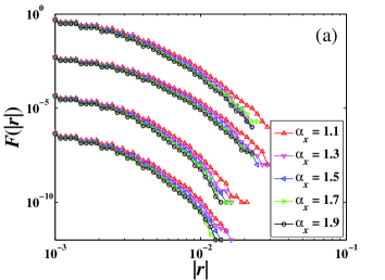
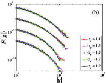
In this case, there are no power-law tails in and we have four combinations for and that are , , , and . For each combination, we investigate five different values of from 1.1 to 1.9 with a step of 0.2. For each value of , our simulations are conducted for 20 repeated rounds. In each round, incoming orders are generated, driving the trading system evolve, and the first 2000 orders are excluded from analysis. The complementary cumulative distribution can be determined for each in every combination. We show the tails of , which is the complementary cumulative probability distribution of , since the return distributions are almost symmetric for positive and negative returns.
The resultant 20 empirical distributions of the trade-by-trade absolute returns for each combination are given in Fig. 1(a). It is evident that there is no power-law tails observed in the distributions. For each combination, the distribution decays faster for larger . We also find that there are more large returns for the two combinations where . This is explained by the two facts that has stronger impact on or equivalently and that a Laplace distribution has heavier tails than a Gaussian. Fig. 1(b) presents the distributions of the standardized returns , where and are respectively the mean and the standard deviation of . It is interesting to observe that the five distributions collapse onto a single curve for all four combinations.
3.3 Case 2: The right part of has a power-law tail with
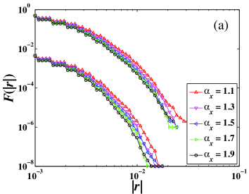
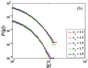
In this case, the right part of has a power-law tail with and we have two combinations for and : and . The simulation procedure is the same as in Section 3.2. The resultant 10 empirical distributions of the trade-by-trade absolute returns for each combination are given in Fig. 2(a). Again, no power-law tails are observed in these distributions. For each combination, the distribution decays faster for larger . We also find that there are more large returns for the the combination where . The same explanation applies. Fig. 2(b) presents the distributions of the normalized returns and the five distributions for each combination collapse remarkably onto a single curve.
3.4 Case 3: The left part of has a power-law tail with
In this case, the left part of has a power-law tail with and we have two combinations for and , which are and . The simulation procedure is the same as in Section 3.2. The resultant empirical distributions of the trade-by-trade absolute returns for each combination are depicted in Fig. 3(a) and (b), respectively. Nice power-law tails are observed in all the distributions. For each combination, the tail exponent increases with . Comparing the distributions in the two plots, no significant difference can be identified in the return distributions with the same value of . In other words, the shape of or equivalently is fully determined by . It is not out of expectation that there is no scaling in the distributions of the normalized returns, , and we thus do not show them here.
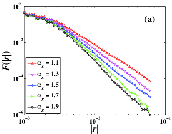
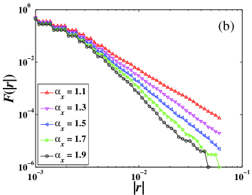
In summary, our simulations confirms that the return distribution is mainly determined by the distribution of the relative prices of incoming orders placed within the order book with . Heavier tail in will result in heavier tails in . Only when has a power-law tail, will have power-law tails.
4 The return distributions at different timescales
We now investigate the return distributions at different timescales for the MF model with the parameters being extracted from real data Mike-Farmer-2008-JEDC . Specifically, the values of model parameters used in this section are the following: , , , , and . We stress that follows the Student distribution in the standard MF model. The simulation procedure is the same as described in the previous section. We consider the normalized returns rather than the returns per se for convenience.
We adopt the mid-price of the best bid and best ask as the logarithmic price at time after a transaction occurs:
| (12) |
where is the event time corresponding to single trades. The event-time return after trades is then defined as the logarithmic price change:
| (13) |
Here we deal with the standardized returns
| (14) |
where and are respectively the mean and the standard deviation of returns . For simplicity, we drop the subscript below.
4.1 Probability distributions of trade-by-trade returns
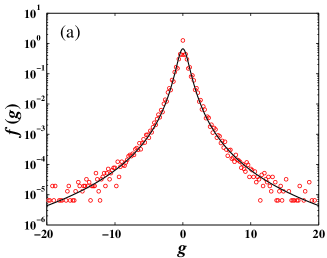
We first focus on . The empirical probability density function is estimated, as shown in Fig. 4(a). We find that can be well modeled by a Student density. Nonlinear least-squares regression gives and . The fitted curve is drawn on the left panel. According to Fig. 4(a), the Student density fits nicely the tails of the empirical density . The fitted model deviates from the empirical density remarkably for small values of . If we amplify the central part for small with finer binning, the shape of looks like a Mexican hat. This is the very character of return distributions of individual stocks caused by the discreteness of price changes in units of tick size. This intriguing structure was reported for common stocks in the US market Plerou-Gopikrishnan-Amaral-Meyer-Stanley-1999-PRE and in the Chinese market Gu-Chen-Zhou-2008b-PA .
For large values of , the Student density function approaches power-law decay in the tails:
| (15) |
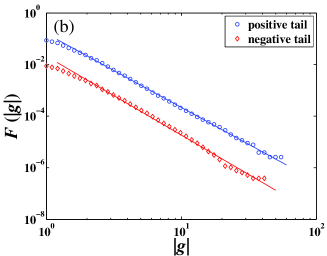
The empirical cumulative distributions of positive and negative are illustrated in Fig. 4(b). Both positive and negative tails decay in a power-law form with and , which are in line with the tail exponent estimated from the Student model. These results indicate that the standardized returns obey the (inverse) cubic law.
4.2 Probability distributions of trade-aggregated returns
We now turn to investigate the distributions of the standardized trade-aggregated returns , where spans several trades. By varying the value of , we are able to compare the PDF’s at different timescales. Specifically, we compare the PDFs for , , and trades with that for trade. As listed in the second column of Table 1, the kurtosis of each PDF is significantly greater than that of the Gaussian distribution whose kurtosis is 3, indicating a much slower decay in the tails. In addition, the kurtosis decreases with respect to the scale . Very similar leptokurtic behavior exists in real stock markets Mantegna-Stanley-2000 .
| Kurtosis | -Gaussian | Positive tail | Negative tail | |||||||
|---|---|---|---|---|---|---|---|---|---|---|
| Scaling range | Scaling range | |||||||||
| 1 | 19.68 | 3.3 | 2.9 | |||||||
| 2 | 19.52 | 3.1 | 3.0 | |||||||
| 4 | 17.06 | 3.2 | 3.1 | |||||||
| 8 | 13.91 | 2.9 | 3.2 | |||||||
| 16 | 10.72 | 2.5 | 3.5 | |||||||
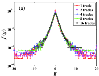
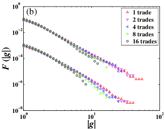
The empirical functions for different time scales are illustrated in Fig. 5(a). We represent the distribution of one-trade returns for comparison. It is evident that the tail is heavier with the decrease of . This phenomenon can also be characterized by the kurtosis of the distributions. We also notice that the PDF for decays slower than exponential. We have fitted the five curves using the Student density model (5) and the estimated parameters and are listed in Table 1. In Fig. 5(b), we study the tail distributions of the normalized returns . It is observed that both positive and negative tails decay in power-law forms. We have estimated the tail exponents, which are also presented in Table 1. Note that the scaling range decreases with increasing , which is also observed for two Korean indexes Lee-Lee-2004-JKPS and 23 individual Chinese stocks Gu-Chen-Zhou-2008b-PA . As expected, the tails that are characterized by their tail exponents decay faster for larger , which is consistent with the behavior of kurtosis.
The results obtained so far show that, the mock stock simulated from the MF model shares striking similarity in the price dynamics with the Chinese stocks Gu-Chen-Zhou-2008b-PA . However, there are also minor discrepancies. First, the tail exponents of the mock stock are less than that of the Chinese stocks with about 0.2. Second, the return distributions are slightly left-skewed while that of the Chinese stocks are slightly right-skewed. It is not clear if these discrepancies stem from the simplicity of the MF model or are just a reflection of the fact that the parameters of the MF model are not extracted from the Chinese stocks. The analysis presented here shows that the MF model is very powerful and universal.
5 Conclusion
In conclusion, we have studied the return distributions of mock stocks in the Mike-Farmer model based on extensive simulations. We found that the power-law tails of the return distribution in the MF model are caused by the power-law tail in the left part of the distribution of the relative prices of incoming orders, no matter the right part has a power-law tail or not. In addition, we found that the distributions of returns in the MF model at different timescales in units of trades can be modeled by Student distributions, whose tail exponents are close to the well-known cubic law and increase with timescale. The behavior of return distributions is comparable to that of the real data.
Acknowledgments:
This work was partly supported by the National Natural Science Foundation of China (Grant No. 70501011), the Fok Ying Tong Education Foundation (Grant No. 101086), and the Program for New Century Excellent Talents in University (Grant No. NCET-07-0288).
References
- [1] R. N. Mantegna, H. E. Stanley, An Introduction to Econophysics: Correlations and Complexity in Finance, Cambridge University Press, Cambridge, 2000.
- [2] R. Cont, Empirical properties of asset returns: Stylized facts and statistical issues, Quant. Financ. 1 (2001) 223–236.
- [3] W.-X. Zhou, A Guide to Econophysics (in Chinese), Shanghai University of Finance and Economics Press, Shanghai, 2007.
- [4] B. B. Mandelbrot, A. J. Fisher, L. E. Calvet, A multifractal model of asset returns, cowles Foundation Discussion Paper No. 1164 (1997).
- [5] E. Calvet, J. Fisher, Forecasting multifractal volatility, J. Econometrics 105 (2001) 27–58.
- [6] T. Lux, The multi-fractal model of asset returns: Its estimation via GMM and its use for volatility forecasting, University of Kiel (2003).
- [7] T. Lux, The Markov-switching multi-fractal model of asset returns: GMM estimation and linear forecasting of volatility, University of Kiel (2004).
- [8] Z. Eisler, J. Kertész, Multifractal model of asset returns with leverage effect, Physica A 343 (2004) 603–622.
- [9] E. Bacry, J. Delour, J.-F. Muzy, Modelling financial time series using multifractal random walks, Physica A 299 (2001) 84–92.
- [10] E. Bacry, J. Delour, J.-F. Muzy, Multifractal random walk, Phys. Rev. E 64 (2001) 026103.
- [11] B. Pochart, J.-P. Bouchaud, The skewed multifractal random walk with applications to option smiles, Quant. Financ. 2 (2002) 303–314.
- [12] R. Cont, J.-P. Bouchaud, Herd behavior and aggregate fluctuations in financial markets, Macroecon. Dyn. 4 (2000) 170–196.
- [13] D. Stauffer, Can percolation theory be applied to the stock market?, Ann. Phys. 7 (1998) 529–538.
- [14] D. Stauffer, T. J. P. Penna, Crossover in the Cont-Bouchaud percolation model for market fluctuations, Physica A 256 (1998) 284–290.
- [15] V. Eguíluz, M. Zimmermann, Transmission of information and herd behavior: An application to financial markets, Phys. Rev. Lett. 85 (2000) 5659–5662.
- [16] R. D’Hulst, G. J. Rodgers, Exact solution of a model for crowding and information transmission in financial markets, Int. J. Theoret. Appl. Financ. 3 (2000) 609–616.
- [17] Y.-B. Xie, B.-H. Wang, H.-J. Quan, W.-S. Yang, P.-M. Hui, Finite-size effect in the Eguíluz and Zimmermann model of herd formation and information transmission, Phys. Rev. E 65 (2002) 046130.
- [18] H. Föellmer, Random economies with many interacting agents, J. Macroecon. 1 (1974) 51–62.
- [19] D. Chowdhury, D. Stauffer, A generalized spin model of financial markets, Eur. Phys. J. B 8 (1999) 477–482.
- [20] G. Iori, Avalanche dynamics and trading friction effects on stock market returns, Int. J. Modern Phys. C 10 (1999) 1149–1162.
- [21] T. Kaizoji, Speculative bubbles and crashes in stock markets: An interacting-agent model of speculative activity, Physica A 287 (2000) 493–506.
- [22] S. Bornholdt, Expectation bubbles in a spin model of markets: Intermittency from frustration across scales, Int. J. Modern Phys. C 12 (2001) 667–674.
- [23] W.-X. Zhou, D. Sornette, Self-organizing Ising model of financial markets, Eur. Phys. J. B 55 (2007) 175–181.
- [24] W. B. Arthur, Inductive reasoning and bounded rationality, Am. Econ. Rev. 84 (1994) 406–411.
- [25] D. Challet, Y.-C. Zhang, Emergence of cooperation and organization in an evolutionary game, Physica A 246 (1997) 407–418.
- [26] D. Challet, M. Marsili, Y.-C. Zhang, Modeling market mechanism with minority game, Physica A 276 (2000) 284–315.
- [27] P. Jefferies, M. L. Hart, P.-M. Hui, N. F. Johnson, From market games to real-world markets, Eur. Phys. J. B 20 (2001) 493–501.
- [28] D. Challet, M. Marsili, Y.-C. Zhang, From minority games to real markets, Quant. Financ. 1 (2001) 168–176.
- [29] D. Challet, M. Marsili, Y.-C. Zhang, Stylized facts of financial markets and market crashes in minority games, Physica A 294 (2001) 514–524.
- [30] D. Challet, M. Marsili, Y.-C. Zhang, Minority games and stylized facts, Physica A 299 (2001) 228–233.
- [31] D. Challet, M. Marsili, Y.-C. Zhang, Minority Games: Interacting Agents in Financial Markets, Oxford University Press, Oxford, 2005.
- [32] T. Lux, M. Marchesi, Scaling and criticality in a stochastic multi-agent model of a financial market, Nature 397 (1999) 498–500.
- [33] S. Maslov, Simple model of a limit order-driven market, Physica A 278 (2000) 571–578.
- [34] M. G. Daniels, J. D. Farmer, L. Gillemot, G. Iori, E. Smith, Quantitative model of price diffusion and market friction based on trading as a mechanistic random process, Phys. Rev. Lett. 90 (2003) 108102.
- [35] J. D. Farmer, P. Patelli, I. I. Zovko, The predictive power of zero intelligence in financial markets, Proc. Natl. Acad. Sci. USA 102 (2005) 2254–2259.
- [36] F. Slanina, Critical comparison of several order-book models for stock-market fluctuations, Eur. Phys. J. B 61 (2008) 225–240.
- [37] S. Mike, J. D. Farmer, An empirical behavioral model of liquidity and volatility, J. Econ. Dyn. Control 32 (2008) 200–234.
- [38] F. Lillo, J. D. Farmer, The long memory of the efficient market, Stud. Nonlin. Dyn. Econometr. 8 (3) (2004) 1–33.
- [39] I. Zovko, J. D. Farmer, The power of patience: A behavioural regularity in limit-order placement, Quant. Financ. 2 (2002) 387–392.
- [40] J.-P. Bouchaud, M. Mézard, M. Potters, Statistical properties of stock order books: empirical results and models, Quant. Financ. 2 (2002) 251–256.
- [41] M. Potters, J.-P. Bouchaud, More statistical properties of order books and price impact, Physica A 324 (2003) 133–140.
- [42] J.-I. Maskawa, Correlation of coming limit price with order book in stock markets, Physica A 383 (2007) 90–95.
- [43] G.-F. Gu, W. Chen, W.-X. Zhou, Empirical regularities of order placement in the Chinese stock market, Physica A 387 (2008) 3173–3182.
- [44] A. Ranaldo, Order aggressiveness in limit order book markets, J. Financ. Markets 7 (2004) 53–74.
- [45] F. Lillo, Limit order placement as an utility maximization problem and the origin of power law distribution of limit order prices, Eur. Phys. J. B 55 (2007) 453–459.
- [46] R. C. Blattberg, N. J. Gonedes, A comparison of the stable and student distributions as statistical models for stock prices, J. Business 47 (2) (1974) 244–280.
- [47] C. Tsallis, C. Anteneodo, L. Borland, R. Osorio, Nonextensive statistical mechanics and economics, Physica A 324 (2003) 89–100.
- [48] V. Plerou, P. Gopikrishnan, L. A. N. Amaral, M. Meyer, H. E. Stanley, Scaling of the distribution of price fluctuations of individual companies, Phys. Rev. E 60 (1999) 6519–6529.
- [49] K. E. Lee, J. W. Lee, Scaling properties of price changes for Korean stock indices, J. Korean Phys. Soc. 44 (2004) 668–671.