Atmospheric, long baseline, and reactor neutrino data constraints on
Abstract
An atmospheric neutrino oscillation tool that uses full three-neutrino oscillation probabilities and a full three-neutrino treatment of the MSW effect, together with an analysis of the K2K, MINOS, and CHOOZ data, is used to examine the bounds on . The recent, more finely binned, Super-K atmospheric data is employed. For km/GeV, we previously found significant linear in terms. This analysis finds bounded from above by the atmospheric data while bounded from below by CHOOZ. The origin of this result arises from data in the previously mentioned very long baseline region; here, matter effects conspire with terms linear in to produce asymmetric bounds on . Assuming CP conservation, we find (90% C.L.).
pacs:
14.60.PqThe phenomenon of neutrino oscillations exp ; k2k ; atmo ; atmor has been observed in a variety of experiments: solar, long baseline (LBL) reactor, atmospheric, and LBL accelerator experiments. Including the constraint imposed by the CHOOZ reactor experiment choo , one may quantitatively determine the three mixing angles and two mass-squared differences that parameterize three-neutrino phenomenology cgg07 . An outstanding question is the value of the mixing angle . Present analyses cgg07 yield . We examine the impact of small effects, particularly those linear in dlde05 ; dlde05b ; ps04 ; choubey , on extracting this small parameter from the data. We find that including the full three-neutrino oscillation probabilities and a full three-neutrino MSW calculation are important for determining this mixing angle.
Knowledge of is a particularly important part of neutrino oscillation phenomenology because its value sets the magnitude of possible CP violating effects and the size of effects that might be used to determine the neutrino mass hierarchy. There are presently three new reactor experiments under development which are designed to measure , Daya Bay DYB , Double CHOOZ dCHO , and RENO RENO , as well as two long baseline experiments, T2K T2K and NOvA nova . The subsequent generation of experiments, e.g., those which will ascertain the level of CP violation, cannot proceed until the current generation better determines the value of .
The standard model of neutrinos conserves flavor, as is required by the data. Neutrino oscillations require adding a posteriori a mass term to the standard model Lagrangian. The standard model Lagrangian is diagonal in flavor; the added mass term is diagonal in the basis which governs vacuum propagation. The relation between the two bases is given by a phenomenological unitary matrix . In the absence of CP violation, it is real. We employ the standard representation pmns written in terms of the three mixing angles, , , and . In vacuum, the probability that a neutrino of flavor and energy will be detected a distance from the source as a neutrino of flavor is given by
| (1) |
with and , where is measured in km, in GeV, and the mass eigenvalues in eV. If (anti-)neutrinos travel an appreciable distance through matter of sufficient density, then one must add to the Hamiltonian an effective potential to account for the (anti-)neutrino–matter interactions msw . This potential yields different effective mixing angles and neutrino masses. For neutrinos which propagate through the earth over long baselines, it is crucial to take such matter effects into account. We do so by using the approach developed in Ref. ohsn . We employ a two density model of the earth: a mantle of density 4.5 gm/cm3 and a core of density 11.5 gm/cm3 with radius 3486 km. This approach incorporate the MSW effect into a three-neutrino framework without the use of approximate oscillation formulae. We note that it is possible for parametric resonances to occur when neutrinos pass between regions of differing densities parametric ; our treatment of matter effects automatically insures that such resonances are fully incorporated.
Atmospheric neutrino experiments are unique in that the baselines span several orders of magnitude making them sensitive to an enormous region of relevant parameter space. However, the SK-atmospheric experiment is the most difficult to model as one must use the detected charged lepton to infer the direction and energy of the incident neutrino. A complete description of our analysis tool can be found in Ref. jesus . Statistical errors are included in the chi-square function whereas systematic errors are accounted for by using the pull method pulls . We include 43 pulls, the most important being the overall flux normalization. We also include jesus a simple model of the multi-ring events. For CHOOZ, K2K, and MINOS, we utilize standard analysis techniques jesus .
We introduce the commonly used “sub-dominant approximation” to provide a comparison for the full three-neutrino treatment. It arises from an expansion in the ratio of the mass-squared differences, . The oscillation probabilities are then given by
| (2) | |||||
Additional correction terms can be added cgg07 ; expans . We effect this approximation by setting in our full three-neutrino code; in this treatment, matter effects will differ slightly from the approximations used by others.
We take the bounds on the mixing angles as and , as suggested in Ref. dlde05c . For no CP violation, this produces an allowed parameter space that is a single connected region. The (equivalent) often used bounds, with Dirac CP phase , produce two disconnected regions.
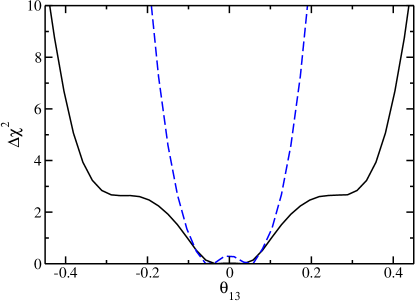
We begin utilizing the sub-dominant approximation. Ref. atmor showed that atmospheric data alone restrict the allowed value of , although less so than does CHOOZ. We use the data from Ref. atmor , which are binned more finely in energy than the original data atmo . In Fig. 1, we plot versus , varying and . The solid [black] curve contains only atmospheric data. Our results quantitatively reproduce those of Ref. atmor which also used the sub-dominant approximation. Both give (or ) for . Reproducing this result is a strong test for our analysis tool. The dashed [blue] curve in Fig. 1 represents for the data set which includes the atmospheric atmor , LBL (K2K and MINOS k2k ), and CHOOZ choo experiments. It is CHOOZ which restricts much more so than the atmospheric data in the sub-dominant approximation.
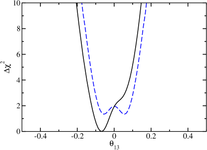
We now compare the sub-dominant approximation with the full three-neutrino calculation. In Fig. 2, we plot for the full data set (atmospheric, LBL, and CHOOZ) using the sub-dominant approximation, dashed [blue] curve, and the full three-neutrino calculation, solid [black] curve. We fix the solar parameters at their best fit values cgg07 , and eV2, as this analysis largely decouples from these two parameters. Note that the sub-dominant results are symmetric about , as is manifest in Eqs. (2). For the full three-neutrino model, the asymmetry about zero is primarily due to terms in the oscillation probabilities which are linear in . We have previously investigated the importance of such terms for very long baselines, km/GeV dlde05 ; dlde05b . Such linear terms and the interference between the and oscillations have also been investigated in Refs. ps04 ; choubey . The importance of this very long baseline region in the atmospheric data has also been noted in Ref. ghosh . Terms linear in are not negligible when extracting the value of this small angle.
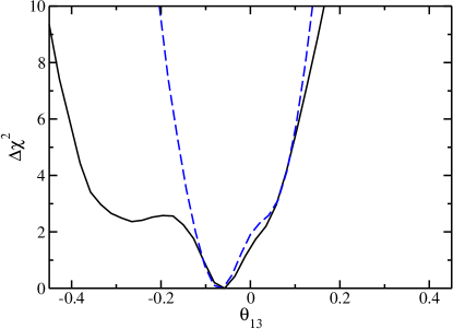
We next examine the contribution of the atmospheric data alone to , the [black] solid curve in Fig. 3. The dashed [blue] curve employs the full data set. For positive , the atmospheric data are more restrictive than even CHOOZ. The restrictions for negative are set by the CHOOZ data. Overall, we find the allowed region for to be asymmetric about zero, bounded from above by atmospheric data and bounded from below by CHOOZ. The final value is at 90% confidence level, corresponding to for a three parameter analysis of this data set. In Fig. 3, we, as have others nzero , find a non-zero value for ; furthermore, we find a statistically insignificant preference for a negative value.
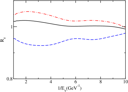
Which subset of atmospheric data results in the strict upper bound on and the lack thereof from below? To answer this, we examine which has . We find that the sub-GeV fully contained events are responsible for two-thirds of this . Furthermore, one-half of the total change in chi-squared (4.5) comes from the single angular bin, , bin II, for fully contained -like events, and the two lowest energy bins in which the charged lepton momentum, , is less than 400 MeV/c. This is well into the very long baseline region mentioned previously where we expect contributions from terms linear in . Bin I, , contains neutrinos which traverse the core suppressing their amplitude of oscillation.
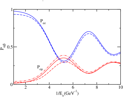
In Fig. 4, we plot oscillation probabilities for angular bin II and the lowest energy bin, MeV/c. The solid curves use the best fit parameters, the dash (dot-dash) curves use . For , the top two [blue] curves, there is only a quadratic term in which lowers . Examining the lower three [red] curves, we see that decreases (increases) with positive (negative) . The number of e-like events measured in an atmospheric experiment is related to with the ratio of the to flux at the source. From Fig. 4, effects due to terms linear in combine constructively for positive and destructively for negative . This is confirmed in Fig. 5 where we compare the effect of positive and negative upon for neutrinos in bin II. Here, we also discover that the excess of e-like events at low energies ps04 results in the strict bound on positive values of in contrast to negative values. The effect is enhanced by an MSW resonance near MeV for a mantle density of 4.5 gm/cm3. Notice that the effect is for bins where the neutrino travels through almost the entire Earth, a distance such that the resonance is fully developed. Previously, the constancy of was found to impose an upper bound on dharam ; here we see that also helps constrain the sign of this mixing angle.
Probing further, we may approximate the e-like events at Super-K for the very LBL sub-GeV data as in Ref. dlde05b
| (3) |
where the superscript refers to the effective parameter values in matter and represents the deviation from maximal mixing, . Note the term linear in is proportional to . At the MSW resonance, , and this mixing angle increases with energy up to . Thus the coefficient of the term in Eq. (3) is negative above the resonant energy so that a negative produces an excess of e-like events. The bounding of from above by the atmospheric data depends critically on incorporating the full MSW effect. For these low energy neutrinos, one has ; the dependence of our results upon this ratio is not severe. More significant is the dependence upon ; the octant of can conspire to enhance or suppress the effect of upon an excess of e-like events.
In this new era of precision neutrino experiments, small effects, such as those arising from , require a careful treatment. Future reactor experiments DYB ; dCHO ; RENO are sensitive to and thus can determine the magnitude of , but not its sign. The long baseline experiments, T2K ; nova will contain small effects that are linear in , while an upgraded Super-K will produce additional data in the region most sensitive to effects linear in . How these different data interplay with each other in determining this mixing angle will be most interesting.
We find that present atmospheric data restrict the value of from above, while the limit from below remains as determined by CHOOZ, and that , assuming no CP violation. It is important to realize first that can be negative dlde05c and, second, that linear effects lead to asymmetric errors. Our analysis requires the use of the more finely binned atmospheric data, Ref. atmor , the use of the full three-neutrino oscillation probabilities, and inclusion of the full MSW effect.
I ACKNOWLEDGMENTS
The work of J. E. R. and D. J. E. is supported, in part, by US Department of Energy Grant DE-FG02-96ER40975; the work of J. E. R. is supported, in part by CONACyT, Mexico; the work of D. C. L. is supported, in part, by US Department of Energy Grant DE-FG02-96ER40989.
References
- (1) Homestake Collaboration, B. T. Cleveland et al., Astrophys. J. 496, 505 (1998); SAGE Collaboration, J. N. Abdurashitov et al., J. Exp. Theor. Phys. 95, 181 (2002); GALLEX Collaboration, W. Hampel et al., Phys. Lett. B 477, 127 (1999); GNO Collaboration, M. Altmann et al., Phys. Lett. B 616, 174 (2005); Super-K Collaboration, M. B. Smy et al., Phys. Rev. D 69, 011104 (2004); SNO Collabortion, S. N. Ahmed et al., Phys. Rev. Lett. 92, 181301 (2004); B. Aharmim et al., Phys. Rev. C 72, 055502 (2005); KamLAND Collaboration, T. Akari et al., Phys. Rev. Lett. 94, 081801 (2005);
- (2) K2K Collaboration, E. Aliu et al., Phy. Rev. Lett. 94, 081802 (2005); MINOS Collaboration, P. Adamson et. al. arXiv:0806.2237 [hep.exp].
- (3) Super-K Collaboration, Y. Ashie et al., Phys. Rev. D 71, 112005 (2005).
- (4) Super-K Collaboration, J. Hosaka et al., Phys. Rev. D 74, 032002 (2006).
- (5) CHOOZ Collaboration, M. Appolonio et al., Eur. Phys. J. C 27, 331 (2003).
- (6) M. C. Gonzalez-Garcia and M. Maltoni, Phys. Rept. 460, 1 (2008).
- (7) D. C. Latimer and D. J. Ernst, Phys. Rev. C 71, 062501(R) (2005).
- (8) D. C. Latimer and D. J. Ernst, Phys. Rev. C 72, 045502 (2005); D. C. Latimer, J. Escamilla, and D. J. Ernst, Phys. Rev. C76, 055502 (2007).
- (9) O. L. G. Peres, A. Yu. Smirnov, Nucl.Phys. B680 (2004) 479.
- (10) S. Choubey and P. Roy, Phys. Rev. D 73, 013006 (2006).
- (11) X. Guo et al. (Daya Bay Collaboration) arXiv:hep-ex/0701029.
- (12) F. Ardellier et al. (Double CHOOZ Collaboration) arXiv:hep-ex/0606025..
- (13) K. K. Joo (RENO Collaboration) Nucl. Phys. B, Proc. Suppl. 168, 125 (2007).
- (14) Y. Oyama (T2K Collaboration) arXiv:hep-wx/0512041.
- (15) See http://www-nova.fnal.gov/
- (16) Z. Maki, M. Nakagawa and S. Sakata, Prog. Theor. Phys. 28, 870 (1962); B. Pontecorvo, Sov. Phys. JETP 26, 984 (1968) [Zh. Eksp. Teor. Fiz. 53, 1717 (1967)].
- (17) L. Wolfenstein, Phys. Rev. D 17, 2369 (1978); S. P. Mikheev and A. Y. Smirnov, Sov. J. Nucl. Phys. 42, 913 (1985) [Yad. Fiz. 42, 1441 (1985)].
- (18) T. Ohlsson and H. Snellman, Phys. Lett. B 474, 153 (2000); J. Math. Phys. 41, 2768 (2000).
- (19) M. Koike, T. Ota, M. Saito and J. Sato, arXiv:0902.1597 [hep-ph]; E. K. Akhmedov, M. Maltoni and A. Y. Smirnov, Phys. Rev. Lett. 95, 211801 (2005); E. K. Akhmedov, A. Dighe, P. Lipari and A. Y. Smirnov, Nucl. Phys. B542, 3 (1999); V. K. Ermilova, V. A. Tsarev and V. A. Chechin, Kr. Soob, Fiz. [Short Notices of the Lebedev Institute] 5, 26 (1986).
- (20) J. E. Roa, D. C. Latimer, and D. J. Ernst, arXiv:0904.3930 [nucl-th]; J. Escamilla Roa, PhD thesis (Vanderbilt University, 2008).
- (21) G. L. Fogli, E. Lisi, A. Marrone, D. Montanino, and A. Palazzo, Phys. Rev. D 66, 053010 (2002).
- (22) E. K. Akhmedov et al., JHEP 0404, 078 (2004).
- (23) D. C. Latimer and D. J. Ernst, Phys. Rev. D 71, 017301 (2005).
- (24) R. Gandhi, P. Ghoshal, S. Goswami, and S. U. Sankar, Phys. Rev. D 78, 073001 (2008).
- (25) A. B. Balantekin and D. Yilmaz, J. Phys. G 35, 075007 (2008); G. L. Fogli, E. Lisi, A. Marrone, A. Palazzo, and A. M. Rotunno, Phys. Rev. Lett. 101, 141801 (2008); arXiv:0905.3549 [hep-ph]; T. Schwetz, M. Tórtola, and J. W. F. Valle, New J. of Phys. 10, 113011 (2008); M. Maltoni and T. Schwetz, arXiv:0812.3161 [hep-ph].
- (26) D. V. Ahluwalia, Mod. Phys. Lett. A 13, 2249 (1998); I. Stancu and D. V. Ahluwalia, Phys. Lett. B460, 431 (1999); D. V. Ahluwalia, Y. Liu, and I. Stancu, Mod. Phys. Lett. A 17, 13 (2002).