Missing energy look-alikes with 100 pb^-1 at the LHC

Abstract

A missing energy discovery is possible at the LHC with the first 100 pb^-1 of understood data. We present a realistic strategy to rapidly narrow the list of candidate theories at, or close to, the moment of discovery. The strategy is based on robust ratios of inclusive counts of simple physics objects. We study specific cases showing discrimination of look-alike models in simulated data sets that are at least 10 to 100 times smaller than used in previous studies. We discriminate supersymmetry models from non-supersymmetric look-alikes with only 100 pb^-1 of simulated data, using combinations of observables that trace back to differences in spin.

I Introduction

I.1 Twenty questions at the LHC

Many well-motivated theoretical frameworks make dramatic predictions for the experiments at the Large Hadron Collider. These frameworks are generally based upon assumptions about new symmetries, as is the case for supersymmetry (SUSY) Wess:1973kz ; Ramond:1971gb and little Higgs (LH)ArkaniHamed:2001nc ; ArkaniHamed:2002qx , or upon assumptions about new degrees of freedom such as extra large ArkaniHamed:1998rs or warped Randall:1999ee spatial dimensions. Within each successful framework, one can construct a large number of qualitatively different models consistent with all current data. Collectively these models populate the “theory space” of possible physics beyond the Standard Model. The BSM theory space is many dimensional, and the number of distinct models within it is formally infinite. Since the data will not provide a distinction between models that differ by sufficiently tiny or experimentally irrelevant details, infinity, in practice, becomes some large finite number $N$. The mapping of these $N$ models into their experimental signatures at the LHC, though still incomplete, has been explored in great detail.

As soon as discoveries are made at the LHC, physicists will face the LHC Inverse Problem: given a finite set of measurements with finite resolutions, how does one map back Binetruy:2003cy -ArkaniHamed:2005px to the underlying theory responsible for the new phenomena? So far, not enough progress has been made on this problem, especially as it relates to the immediate follow-up of an early LHC discovery.

When $N$ is large, it is not a viable strategy to discriminate between $N$ alternative explanations by performing $N$ tests. However, as the game “twenty questions” illustrates, a well-designed series of simple tests can identify the correct alternative in of order log($N$) steps, proceeding along a decision tree such that, at each branching, of order half of the remaining alternatives are eliminated.

Addressing the LHC Inverse Problem implies designing and implementing this series of simple tests in the LHC experiments, so that with high confidence a significant fraction of the remaining theory space is ruled out at each step. The results of the first few tests will shape the requirements for future tests, so the immediate need is to develop the strategy for the early tests. In this paper we provide this strategy for the case of an LHC discovery in the inclusive missing energy signature.

I.2 Missing energy at the LHC

The existence of dark matter provides a powerful motivation to explore missing energy signatures at the LHC, under the assumption that a significant fraction of dark matter may consist of weakly interacting thermal relics. Missing energy at the LHC is experimentally challenging. Most of the energy of 14 TeV $pp$ collisions is carried off by undetected remnants of the underlying event, so missing energy searches actually look for missing transverse energy ($E_{T}^{\rm{miss}}$) of the partonic subprocess. $E_{T}^{\rm{miss}}$ searches are plagued by instrumental and spurious backgrounds, including cosmic rays, scattering off beam halo and jet mismeasurement. Standard Model processes create an irreducible $E_{T}^{\rm{miss}}$ background from processes such as the $Z$ boson decay to neutrinos and $t\bar{t}$ production followed by semileptonic decays of the top.

In many theoretical frameworks with dark matter candidates, there are heavy strongly interacting particles with the same conserved charge or parity that makes the dark matter particle stable. These colored particles will be pair-produced at the LHC with cross sections roughly in the range 0.1 to 100 pb. Their subsequent decays will produce Standard Model particles along with a pair of undetected dark matter particles. Thus the generic experimental signature is both simple and inclusive: large $E_{T}^{\rm{miss}}$ accompanied by multiple energetic jets. A detailed strategy for early discovery with the inclusive $E_{T}^{\rm{miss}}$ signature was presented in the CMS Physics Technical Design Report Ball:2007zza -Spiropulu:2008ug and studied with full simulation of the CMS detector. After a series of cleanup and analysis cuts on a simulated $E_{T}^{\rm{miss}}$ trigger sample targeting the reduction of the instrumental and physics backgrounds, the signal efficiency remained as high as 25%. These results indicate that, for signal cross sections as low as a few pb, an $E_{T}^{\rm{miss}}$ discovery could be made with the first 100 pb^-1 of understood LHC data. In our study we assume as the starting point that a greater than $5\sigma$ excess of events will be seen in a 14 TeV LHC data sample of 100 pb^-1 with an inclusive missing energy analysis. For invariability and comparability we effectively adopt the full analysis path and requirements used in Ball:2007zza .

I.3 Look-alikes at the moment of discovery

At the moment of discovery a large number of theory models will be immediately ruled out because, within conservative errors, they give the wrong excess. However a large number of models will remain as missing energy look-alikes, defined as models that predict the same inclusive missing energy excess, within some tolerance, in the same analysis in the same detector, for a given integrated luminosity. The immediate challenge is then to begin discriminating the look-alikes.

The look-alike problem was studied in ArkaniHamed:2005px as it might apply to a later mature phase of the LHC experiments. Even restricted to the slice of theory space populated by a partial scan of the MSSM, ignoring SM backgrounds and systematic errors, and applying an uncorrelated $\chi^{2}$-like statistical analysis to 1808 correlated observables, this study found that a large number of look-alikes remained unresolved in a simulation equivalent to 10 fb^-1. A more recent analysis Berger:2007ut attempts to resolve these look-alikes in a simulation of a future linear collider.

At the moment of an early discovery the look-alike problem will be qualitatively different. The data samples will be much smaller, with a limited palette of robust reconstructed physics objects. For example, $\tau$ or $b$ tagging in multijet final states will be in development during the 100 pb^-1 era. In many small data samples peaks and edges in invariant mass distributions may not be visible, and most observables related to detailed features of the events will be rate limited. The observables that are available to discriminate the look-alikes in the very early running will be strongly correlated by physics and systematics making it imprudent to combine them in a multivariate analysis.

I.4 Is it SUSY?

By focusing on the discrimination of look-alikes, we are pursuing a strategy of simple binary choices: is Model A a significantly better explanation of the discovery data set than Model B? Each answer carries with it a few bits of important fundamental information about the new physics process responsible for missing energy. Obviously we will need to make many distinct look-alike comparisons before we can hope to build up a clear picture from these individual bits.

Consider how this strategy might play out for answering the basic question “is it SUSY?” It may not be possible to answer this question conclusively during the 100 pb^-1 era. Our strategy will consist of asking a series of more modest questions, some of them of the form: “does SUSY Model A give a significantly better explanation of the discovery data set than non-SUSY Model B?” None of these individual bits of information by itself is equivalent to answering “is it SUSY?” However we demonstrate that we can build up a picture from the data that connects back to features of the underlying theory.

Furthermore, we demonstrate a concrete method to obtain indirect information about the spin of the new particles. We establish how to discriminate between a non-SUSY model and its SUSY look-alikes. Even though we cannot measure the spins of the exotic particles directly, spin has significant effects on production cross sections, kinematic distributions and signal efficiencies. We are thus able to discriminate SUSY from non-SUSY using combinations of observables that trace back to differences in spin. Our study shows that in favorable cases this can be accomplished with data sets as small as 100 pb^-1.

I.5 Outline

In section II we review in detail the missing energy discovery path, including the experimental issues and systematics that limit our ability to fully reconstruct events from the discovery data set. We explain how the missing energy signals are simulated, and the uncertainties associated with these simulations. In section III we discuss the problem of populating the parts of the theory space relevant to a particular missing energy discovery. In section IV we introduce two groups of look-alike models relative to two different missing energy signals. For models differing only by spins, we discuss how cross sections, kinematic distributions and efficiencies can be used to distinguish them, drawing from formulae developed in the Appendix. In section V we define all of the robust observables that we use to discriminate among the look-alikes, and in section VI we describe the look-alike analysis itself and how we compute the significance of the discriminations. Sections VII and VIII give a summary of our results, with details relegated to further Appendices. Finally section IX describes the steps we are following to improve this analysis for use with real data.

II Discovery analysis for missing energy

Missing energy hadron collider data has been used previously for successful measurements of Standard Model processes with energetic neutrinos; these include the $Z^{0}$ boson invisible decay rates, the top quark cross section, searches for the Higgs boson Acosta:2005ga and a precise extraction of the $W$ mass from the reconstruction of the $W$ transverse mass Abe:1995np . Pioneering searches for new phenomena in missing energy data sets at the Tevatron Spiropulu:2000nb -Affolder:2000ef led to the development and understanding of the basic techniques that will be used in missing energy searches at the LHC.

In an ideal detector, with hermetic 4$\pi$ solid angle coverage and excellent calorimeter resolution, the measurement of missing energy is the measurement of the neutrino energy and the energy of any other neutral weakly interacting particles. In a real detector it is also a measurement of the energy that escapes detection due to uninstrumented regions and other detector effects such as imperfect calorimeter response. Muons are sources of missing energy since a muon typically deposits only of order a few GeV of its total energy in the calorimeters. QCD jets produce real $E_{T}^{\rm{miss}}$ from semileptonic decays of heavy flavor, and fake $E_{T}^{\rm{miss}}$ from detector-induced mismeasurements. Thus the $E_{T}^{\rm{miss}}$  distribution of a pure QCD multijet sample has a long tail related to non-Gaussian tails in the detector response. This gives rise to an important background to missing energy searches that is difficult to estimate prior to data. At the Tevatron it has been shown that this background can be brought under control by exploiting the fact that the fake $E_{T}^{\rm{miss}}$ from jet mismeasurements is highly correlated with the azimuthal directions of the leading jets Spiropulu:2000nb .

There are other important sources of fake $E_{T}^{\rm{miss}}$ at hadron colliders, including beam halo induced $E_{T}^{\rm{miss}}$, cosmic ray muons, noise in the data acquisition system, and misreconstruction of the primary vertex. Eliminating these sources requires unbiased filters based on clean definitions of event quality.

To design a missing energy analysis, we need to have some idea of the source of the $E_{T}^{\rm{miss}}$ in the signal. The possibilities include:

• The $E_{T}^{\rm{miss}}$ is entirely from neutrinos. This could arise from the direct decay of new heavy particles to neutrinos, or decays of new heavy particles to top, $W$’s, $Z$’s or $\tau$’s. One appropriate discovery strategy for this case is to look for anomalies in the energetic tails of data sets with reconstructed top, $W$’s or $Z$’s.

• The $E_{T}^{\rm{miss}}$ originates from a single weakly interacting exotic particle in the final state. An example of this possibility is graviton production in models with large extra dimensions Hewett:2002hv . If strong production occurs, the signal will consist predominately of monojets and large $E_{T}^{\rm{miss}}$. Successful analyses for this case were carried out at the Tevatron Acosta:2003tz ; Abazov:2003gp . Other signals that fit this case arise from unparticle models Cheung:2007zza and from models with $s$-channel resonances that have invisible decays.

• The $E_{T}^{\rm{miss}}$ originates from many weakly interacting exotic particles. This can be the case in hidden valley models Strassler:2006im , where the weakly interacting exotics are light pions of the hidden sector. This case is experimentally challenging.

• The $E_{T}^{\rm{miss}}$ originates from two weakly interacting exotic particles in the final state. This is the case for supersymmetry models with conserved $R$ parity, where the weakly interacting particles are neutralino LSPs. It also applies for more generic models with WIMP dark matter candidates.

We focus on a discovery analysis developed for the last case. Thus we are interested in signal events with two heavy WIMPs in the final state. For early discovery at the LHC, the signal events should have strong production cross sections; we will assume that each WIMP arises from the decay of a strongly interacting heavy parent particle. The most generic signature is therefore large $E_{T}^{\rm{miss}}$ in association with at least two high $E_{T}$ jets. There will be additional jets if the WIMP is not produced in a 2-body decay of the parent particle. Furthermore, there is a significant probability of an extra jet from QCD radiation, due to the large phase space. Thus it is only slightly less generic to design an inclusive analysis for large $E_{T}^{\rm{miss}}$ in association with three or more energetic jets. We will refer to this as the inclusive missing energy signature.

In the basic $2\rightarrow 2$ hard scattering, the heavy parent particles of the signal will be produced back-to-back in the partonic subprocess center-of-mass frame; typically they will have $p_{T}$ roughly comparable to their mass $m_{\rm p}$. The WIMPs of mass $m_{\rm dm}$ resulting from the parent particle decays will fail to deposit energy $\geq m_{\rm dm}$ in the calorimeters; if the WIMPS have fairly large $p_{T}$, a significant fraction of this energy contributes to the $E_{T}^{\rm{miss}}$. Thus either large $m_{\rm p}$ or large $m_{\rm dm}$ leads to large $E_{T}^{\rm{miss}}$. Note the azimuthal directions of the WIMPS are anticorrelated, a feature inherited from their parents, so the magnitude of the total $E_{T}^{\rm{miss}}$ tends to be less than the magnitude of the largest single contribution.

At the LHC, the most important Standard Model sources of large real $E_{T}^{\rm{miss}}$ will be $t\bar{t}$, single top, $W$ and $Z$ plus jets associated production, dibosons and heavy flavor decays. Most of these processes produce a hard lepton in association with the $E_{T}^{\rm{miss}}$ from an energetic neutrino. The exception is $Z\rightarrow\nu\bar{\nu}$. Even with a perfect detector, $Z\rightarrow\nu\bar{\nu}$ plus jets is an irreducible physics background.

II.1 Analysis path

In the real data this search will be performed starting from a primary data set that includes requirements of missing energy, jets and general calorimetric activity at the trigger path; the trigger efficiency should be measured in other data samples.

For the offline analysis, we will adopt the inclusive missing energy benchmark analysis studied with the full detector simulation for the CMS Physics Technical Design Report Ball:2007zza ; Yetkin:2007zz .

The first phase is a preselection based on the event quality. The purpose of this primary cleanup is to discard events with fake $E_{T}^{\rm{miss}}$ from sources such as beam halo, data acquisition noise and cosmic ray muons. To eliminate these types of backgrounds the benchmark analysis uses jet variables, averages them over the event to define corresponding event variables, and uses these to discriminate real $E_{T}^{\rm{miss}}$+ multijet events from spurious backgrounds. The event electromagnetic fraction (EEMF) is defined to be the $E_{T}$ weighted jet electromagnetic fraction. We define an event charged fraction (ECHF) as the event average of the jet charged fraction (defined as the ratio of the $\sum{p}_{T}$  of the tracks associated with a jet over the total calorimetric jet $E_{T}$). The preselection also has a quality requirement for the reconstructed primary vertex.

Events that are accepted by the preselection requirements proceed through the analysis path if they have missing transverse energy $E_{T}^{\rm{miss}}$$\geq 200$ GeV and at least three jets with $E_{T}$$\geq 30$ GeV within pseudorapidity $|\eta|<3$. These requirements directly define the missing energy signal signature. In addition the leading jet is required to be within the central tracker fiducial volume i.e. $|\eta|<1.7$. Everywhere in this paper “jets” means uncorrected (raw) jets with $E_{T}$$>30$ GeV and $|\eta|<3$ as measured in the calorimeters; the jet reconstruction is with a simple iterative cone algorithm with a 0.5 cone size in the $\eta-\phi$ space. The missing energy is uncorrected for the presence of muons in the event.

The rest of the analysis path is designed based on elimination of the major backgrounds. The QCD background from mismeasured jets is reduced by rejecting events where the $E_{T}^{\rm{miss}}$ is too closely correlated with the azimuthal directions of the jets. To reduce the large background from $W(\rightarrow\ell\nu)+$jets, $Z(\rightarrow\ell\ell)+$jets and $t\bar{t}$ production an indirect lepton veto (ILV) scheme is designed that uses the tracker and the calorimeters. The ILV retains a large signal efficiency while achieving a factor of two rejection of the remaining $W$ and $t\bar{t}$ backgrounds. The veto is indirect because we don’t identify leptons– instead events are rejected if the electromagnetic fraction of one of the two leading jets is too large, or if the highest $p_{T}$ track of the event is isolated. The signals we are interested in are characterized by highly energetic jets while leptons in the signal originate from cascade decays of the parents or semileptonic $B$ decays in the jets; thus even when a signal event has leptons it is relatively unlikely to be rejected by the ILV. For the models in our study, approximately 85% of all signal events and 70% of signal events with muons or taus pass the ILV cut.

The final selections require that the leading jet has $E_{T}>180$ GeV, and that the second jet has $E_{T}>110$ GeV. We also require $H_{\mathrm{T}}>500$ GeV, where

$$H_{\mathrm{T}}=\sum_{i=2}^{4}E_{T}^{i}+E_{\mathrm{T}}^{\mathrm{miss}}\;,$$ (1)

where the $E_{T}$  is summed over the second, third and fourth (if present) leading jets. These cuts select for highly energetic events, greatly favoring events with new heavy particles over the Standard Model backgrounds.

Table 1 summarizes the benchmark analysis path. The table lists the cumulative efficiencies after each selection for a benchmark signal model and the Standard Model backgrounds. The signal model is the CMS supersymmetry benchmark model LM1, which has a gluino with mass 611 GeV and squarks with masses around 560 GeV. The last line of the table shows the expected number of events that survive the selection in a data set corresponding to 1000 pb^-1 of integrated luminosity. For the QCD background and the single top background, which are not shown in the table, the estimated number of remaining events is 107 and 3, respectively. Thus the total estimated Standard Model background after all selections is 245 events per 1000 pb^-1.

Table 1: Cumulative selection efficiency after each requirement in the $E_{T}^{\rm{miss}}$+ multijets analysis path for a low mass SUSY signal and the major Standard Model backgrounds (EWK refers to $W/Z$,$WW/ZZ/ZW$), see Ball:2007zza ; Yetkin:2007zz ).

Cut/Sample	Signal	$t\bar{t}$	$Z(\rightarrow\nu\bar{\nu})+$ jets	EWK + jets
All (%)	100	100	100	100
Trigger	92	40	99	57
$E_{T}^{\rm{miss}}$$>200$ GeV	54	0.57	54	0.9
PV	53.8	0.56	53	0.9
$N_{j}\geq$3	39	0.36	4	0.1
$|\eta_{d}^{j1}|\geq 1.7$	34	0.30	3	0.07
EEMF $\geq$ 0.175	34	0.30	3	0.07
ECHF $\geq$ 0.1	33.5	0.29	3	0.06
QCD angular	26	0.17	2.5	0.04
$Iso^{lead\;trk}=0$	23	0.09	2.3	0.02
$EMF(j1),$
$EMF(j2)\geq 0.9$	22	0.086	2.2	0.02
$E_{T,1}>$ 180 GeV,
$E_{T,2}>$ 110 GeV	14	0.015	0.5	0.003
$H_{T}>500$ GeV	13	0.01	0.4	0.002
events remaining per 1000 pb-1
	6319	54	48	33

II.2 Triggers and “boxes”

Having established a benchmark analysis path, we also need to define benchmark data samples. With the real LHC data these will correspond to data streams and data paths from various triggers. For the inclusive missing energy signature relevant triggers are the $E_{T}^{\rm{miss}}$ and jet triggers. A single lepton trigger is also of interest, since many models produce energetic leptons in association with large $E_{T}^{\rm{miss}}$. For our study we have chosen simple but reasonable Sphicas:2002gg ; Dasu:2000ge parametrizations of the trigger efficiencies defining our four benchmark triggers :

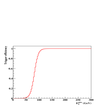
• The MET trigger is a pure inclusive $E_{T}^{\rm{miss}}$ trigger. It is 50% efficient for $E_{T}^{\rm{miss}}$$>80$ GeV, as seen in Figure 1.

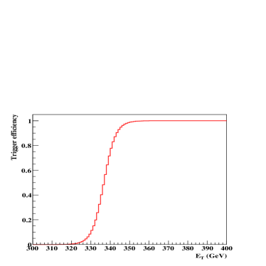
• The DiJet trigger requires two very high $E_{T}$ jets. It is 50% efficient for uncorrected jet $E_{T}$$>340$ GeV, as seen in Figure 2.

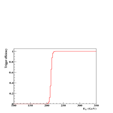
• The TriJet trigger requires three high $E_{T}$ jets. It is 50% efficient for uncorrected jet $E_{T}$$>210$ GeV, as seen in Figure 3.

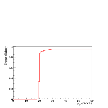
• The Muon20 trigger requires an energetic muon that is not necessarily isolated. The trigger is 88% efficient for muons with $p_{T}=20$ GeV/$c$, asymptoting to 95% as seen in Figure 4.

After applying the selection requirements, these four triggers define four potential discovery data sets. In our simulation the DiJet, TriJet, and Muon20 data sets, after the inclusive missing energy analysis path is applied, are all subsets of the MET sample, apart from one or two events per 1000 pb^-1 . Thus the MET is the largest, most inclusive sample. We perform one complete analysis based on the MET trigger. The other three triggers are then treated as defining three more boxes, i.e. experimentally well-defined subsets of the MET discovery data set. The simplest physics observables are the counts of events in each box.

Figure 1: The $E_{T}^{\rm{miss}}$ trigger efficiency.

Figure 2: The DiJet trigger efficiency.

Figure 3: The TriJet trigger efficiency.

Figure 4: The Muon20 trigger efficiency.

II.3 Backgrounds and systematics

In the CMS study the total number of Standard Model background events remaining after all selections is 245 per 1000 pb^-1 for an $E_{T}^{\rm{miss}}$ trigger sample. The error on this estimate is dominated by i) the uncertainty in how well the detector simulation software simulates the response of the actual CMS detector, and ii) the uncertainty on how well the Standard Model event generators emulate QCD, top production, and $W/Z$ plus jets production. Detailed studies of the real LHC data will be required in order to produce reliable estimates of these uncertainties.

Prior to data we assign conservative error bars on these background projections. We have checked that 100 pb^-1 of data in the MET trigger sample is sufficient for a 5$\sigma$ discovery for the eight models in our study, even if we triple the backgrounds quoted above and include a 15% overall systematic error. The look-alike analysis will be degraded, however, in the event that the Standard Model backgrounds turn out to be much larger than current estimates.

Prior to data, it is also difficult to make a reliable estimate of the main systematic uncertainties that will affect the inclusive missing energy analysis. Systematic uncertainties will decrease over time, as the detectors are better understood, calibration studies are performed, and Standard Model physics is analyzed with the LHC data. For our study we have assumed that, at the moment of discovery, the dominant systematic errors in the full discovery data set will come from three sources:

• Luminosity uncertainty: it affects the counting of events. This systematic uncertainty is process independent.

• Detector simulation uncertainty: it mainly affects calorimetry-related variables in our study, in particular jet counting and the missing energy. This systematic is partially process dependent.

• QCD uncertainty: it includes the uncertainties from the parton distribution functions, higher order matrix elements, and large logarithms. This uncertainty affects event counting, jet counting and the shapes of kinematic distributions. It is partially process dependent.

Note that, since we use uncorrected jets, we do not have a systematic from the jet energy scale. This is traded for a portion of the detector simulation uncertainty, i.e. how well we can map signal events into uncorrected jets as would be measured in the real detector.

II.4 Simulation of the signals

A realistic study of look-alikes requires full detector simulation. For the initial phase of this work a generator level analysis is attractive, being computationally less intensive and providing a clear link between observables and the underlying theory models.

In a generator level analysis, jets are reconstructed by applying a standard algorithm to particles rather than to calorimeter towers. This obviously does not capture the effects of a realistic calorimeter response, calorimeter segmentation, and energy losses due to material in the tracker as well as magnetic field effects.

A compromise between the full simulation and a generator level analysis is a parameterized detector simulation. For the LHC the publicly available software packages include AcerDET RichterWas:2002ch , and PGS pgs . In such a simulation, electrons, muons and photons can be reconstructed using parameterized efficiencies and resolutions based on abstract but educated rules-of-thumb for modern multipurpose detectors. Jets are reconstructed in a virtual calorimeter, from particle energies deposited in cells that roughly mimic the segmentation of a real calorimeter. Calorimeter response is approximated by performing a Gaussian smearing on these energy deposits. The $E_{T}^{\rm{miss}}$ is reconstructed from the smeared energies in these virtual towers.

We performed a preliminary study by comparing PGS results to the full simulation results reported for the SUSY benchmark model LM1 Ball:2007zza ; Yetkin:2007zz . We found that PGS jets are not a good approximation of uncorrected jets in the full simulation, even for the most basic properties such as the $E_{T}$ spectrum. Varying the parameters and adding simple improvements, such as taking into account the 4 Tesla field in the barrel, did not change this conclusion. PGS jets have a behavior, not surprisingly, that is intermediate between generator level jets and uncorrected full simulation jets.

We developed a modified simulation called PGSCMS with the geometry and approximate magnetic field of the CMS detector. The PGS Gaussian smearing and uninstrumented effects in the calorimeters are turned off. Electrons, muons and photons are extracted at generator level, and PGS tau reconstruction is not used. Track information is extracted as in the standard PGS. The calorimeter output improves on a generator level analysis in that we include approximations to the effects of segmentation and the 4 Tesla field, as well as an $\eta$ correction derived from the $z$ value of the primary vertex. We parameterized the detector response in a limited set of look-up tables as a function of the generator-level quantities.

At the analysis level we apply parameterized corrections and reconstruction efficiencies inspired by the published CMS detector performance Bayatian:2006zz . For the jets, we apply an $E_{T}$ and $\eta$ dependent rescaling of their $E_{T}$, tuned to reproduce the full simulation LM1 results in Ball:2007zza ; Yetkin:2007zz . This rescaling makes the jets softer (i.e. takes into account the detector reconstruction): a 50 GeV generator level jet becomes an approximately 30 GeV raw jet in our analysis.

The $E_{T}^{\rm{miss}}$ reconstructed from PGSCMS is essentially identical, modulo small calorimeter segmentation effects, to a a generator level analysis, i.e. our $E_{T}^{\rm{miss}}$ is virtually indistinguishable from the Monte Carlo truth $E_{T}^{\rm{miss}}$ obtained from minus the vector sum of the $E_{T}$ of neutrinos, muons and the other weakly interacting particles (such as the LSP). We did not attempt to rescale the $E_{T}^{\rm{miss}}$; this is a complicated task since $E_{T}^{\rm{miss}}$ is a vector and in general energy losses, calorimeter response and mismeasurements tend to decrease the real large $E_{T}^{\rm{miss}}$ tails while increasing the $E_{T}^{\rm{miss}}$ tails in the distribution of non-real $E_{T}^{\rm{miss}}$ events. Instead of attempting to rescale the $E_{T}^{\rm{miss}}$ event by event, we raised the $E_{T}^{\rm{miss}}$ cut in our benchmark analysis to 220 GeV.

Because of the limitations of our fast simulation, we also simplified parts of the benchmark analysis. The first phase primary cleanup is dropped since it is related to supression of spurious processes that we do not simulate, and it is nearly 100% efficient for the signal. We also drop the jet electromagnetic fraction cuts of the ILV, because they are nearly 100% efficient for the signal.

The resulting performance of our parameterized fast simulation for the SUSY benchmark model LM1 is shown in Table 2. The agreement with the full simulation study is very good. The largest single cut discrepancy is 2%; this occurs for the QCD angular cuts, reflecting the expected fact that our fast simulation does not accurately reproduce jet mismeasurement effects. Since the final efficiencies agree to within 7%, it is plausible that look-alikes defined in our fast simulation study will remain look-alikes in our upcoming full simulation study.

It is important to note that this fast simulation does not reproduce the Standard Model background efficiencies shown in Table 1. In fact the discrepancies in the total efficiencies can approach an order of magnitude. This is to be expected. We are cutting very hard on the Standard Model events, thus the events that pass are very atypical. This is in contrast to the signal events, where the fraction that pass are still fairly generic, and their $E_{T}$ and $E_{T}^{\rm{miss}}$ spectra near the cuts are less steeply falling than those of the background. Since SM backgrounds cannot be estimated from a PGS level analysis, we take our backgrounds from the state-of-the-art analysis in Ball:2007zza ; this approach only works because we have also matched the analysis path used in Ball:2007zza .

The full software chains we use in our study are summarized in Table 3. All of the simulated data sets include an average of 5 pileup events added to each signal event, corresponding to low luminosity LHC running ($\sim 10^{33}$ cm^-2s^-1).

Table 2: Comparison of cut-by-cut selection efficiencies for our $E_{T}^{\rm{miss}}$ analysis applied to the SUSY benchmark model LM1. “Full” refers to the full simulation study Ball:2007zza ; Yetkin:2007zz ; “Fast” is what we obtain from our parameterized fast simulation.

Cut/Software	Full	Fast
Trigger and
$E_{T}^{\rm{miss}}$$>200$ GeV	53.9%	54.5%
$N_{j}\geq$3	72.1%	71.6%
$|\eta_{d}^{j1}|\geq 1.7$	88.1%	90.0%
QCD angular	75.6%	77.6%
$Iso^{lead\;trk}=0$	85.3%	85.5%
$E_{T,1}>$ 180 GeV,
$E_{T,2}>$ 110 GeV	63.0%	63.0%
$H_{T}>500$ GeV	92.8%	93.9%
Total efficiency	12.9%	13.8%

Table 3: Summary of software chains used in this study. The little Higgs spectrum is based on Hubisz:2005tx . PGSCMS is a variation of PGS v4 pgs .

Software/Models	Group 1 models	Group 2 models
Spectrum generator	Isajet v7.69 isajet or	private little Higgs
	or SUSY-HIT v1.1 Djouadi:2006bz	or SuSpect v2.34 Djouadi:2002ze
Matrix element calculator	Pythia v6.4 Sjostrand:2006za	MadGraph v4 madgraph
Event generator	Pythia v6.4	MadEvent v4 madevent
		with BRIDGE bridge
Showering and hadronization	Pythia v6.4	Pythia v6.4
Detector simulation	PGSCMS v1.2.5	PGSCMS v1.2.5
	plus parameterized	plus parameterized
	corrections	corrections

III Populating the theory space

In Section II we gave a partial classification of BSM models according to how many new weakly interacting particles appear in a typical final state. Our benchmark $E_{T}^{\rm{miss}}$ analysis is optimized for the case of two heavy weakly interacting particles per event, as applies to SUSY models with conserved $R$ parity, little Higgs models with conserved $T$ parity and Universal Extra Dimensions models with conserved $KK$ parity. This study is a first attempt at constructing groups of look-alike models drawn from this rather large fraction of the BSM theory space, and developing strategies to discriminate them shortly after an initial discovery.

One caveat is that models from other corners of the theory space may also be look-alikes of the ones considered here. For example, models with strong production of heavy particles that decay to boosted top quarks can produce higher $E_{T}$ jets and larger $E_{T}^{\rm{miss}}$ from neutrinos than does Standard Model top production. Such look-alike possibilities also require study, but they are not a major worry since our results show that we have some ability to discriminate heavy WIMPS from neutrinos even in small data sets.

III.1 SUSY

In a large class of supersymmetry models with conserved $R$ parity, not necessarily restricted to the MSSM, the LSP is either the lightest neutralino or a right-handed sneutrino.

In addition, if the NLSP is a neutralino or sneutrino and the LSP is a gravitino, the $E_{T}^{\rm{miss}}$ signature is the same. Models based on gravity-mediated, gauge-mediated or anomaly-mediated SUSY breaking all provide many candidate models.

Because this relevant portion of SUSY theory space is already so vast, there is a temptation to reduce the scope of the LHC Inverse Problem by making explicit or implicit theoretical assumptions. To take an extreme, one could approach an early LHC discovery in the $E_{T}^{\rm{miss}}$ channel having already made the assumptions that (i) the signal is SUSY, (ii) it has a minimal Higgs sector (MSSM), (iii) it has gravity-mediated SUSY breaking (SUGRA), (iv) the breaking is minimal (mSUGRA) and (v) 100% of dark matter is thermal relic LSPs with an abundance given by extrapolating standard cosmology back to the decoupling epoch. We don’t want to make any such assumptions; rather we want to test theoretical hypotheses in the LHC discovery data set combined with other measurements.

For SUSY we have the benefit of more than one spectrum calculator that can handle general models, more than one matrix element calculator and event generation scheme, and a standardized interface via the SUSY Les Houches Accord (SLHA) SLHA . There are still a few bugs in this grand edifice, but the existing functionality combined with the ability to perform multiple cross-checks puts us within sight of where we need to be when the data arrives.

III.2 Little Higgs

Little Higgs models are a promising alternative to weak scale supersymmetry ArkaniHamed:2002qy -Carena:2006jx . In little Higgs models, the Higgs is an approximate Goldstone boson, with global symmetries protecting its mass (which originates from a quantum level breaking of these symmetries) from large radiative corrections. Many of these LH models require an approximate $T$ parity discrete symmetry to reconcile LH with electroweak precision data. This symmetry is similar to $R$ parity in SUSY models. The new LH particles that would be produced at the LHC would be odd under this symmetry, enforcing the stability of the lightest particle that is odd under $T$ parity. This new particle is weakly interacting and would manifest itself as missing energy at the LHC.

Just as in SUSY, new colored particles are the dominant production modes. These particles subsequently generate high multiplicity final states through decay chains that end with the lightest $T$ odd particle. In LH models, the strongly coupled particles are $T$ odd quarks (TOQ’s), analogous to the squarks of SUSY. The weakly coupled analogues of the gauginos are $T$ odd spin one vector bosons (TOV’s). In the models considered to date, there is no analog of the gluino: this is an important consideration in constructing supersymmetric look-alikes of LH models.

In this study, we work with a minimal implementation of a little Higgs model with $T$ parity that is known as the littlest Higgs model with $T$ parity. This model is based on a $SU(5)/SO(5)$ pattern of global symmetry breaking. Each SM particle except the gluon has an associated LH partner odd under $T$ parity. There is also an extra pair of top partners, one $T$ odd and the other $T$ even, as well as singlets. The lightest $T$ odd particle in this model we label $A_{H}$. It is a heavy gauge boson that is an admixture of a heavy copy of the hypercharge gauge boson and a heavy $W^{3}$ boson.

For event generation, we use a private implementation of the littlest Higgs model within MadGraph. There is a need to generalize this to a wider class of models.

III.3 Universal extra dimensions

Universal extra dimensions models are based on orbifolds of one or two TeV^-1 size extra spatial dimensions Appelquist:2000nn -Dobrescu:2007ec . The five-dimensional version of UED is the simplest. At the first level of Kaluza-Klein ($KK$) excitations, each Standard Model boson has an associated partner particle, and each Standard Model fermion has two associated partner particles (i.e. a vector-like pair). These $KK$ partners are odd under a $KK$ parity, the remnant of the broken translational invariance along the fifth dimension. This parity is assumed to be an exact symmetry. After taking into account mass splittings due to Standard Model radiative corrections, one finds that the lightest $KK$ odd partner is naturally the weakly interacting partner of the hypercharge gauge boson. A wide variety of spectra for the $KK$ odd partners can be obtained by introducing additional interactions that are localized at the orbifold fixed points; these choices distinguish generic UED from the original minimal model of Appelquist:2000nn . These models resemble SUSY.

A public event generation code based on a modification of Pythia is available for generic 5-dimensional UED models Allanach:2006fy . There is a need to generalize this to a wider class of models, e.g. 6-dimensional UED. In our study we have not used any UED examples, but we will include them in the future.

Figure 5: The mass spectra of the MSSM models LM2p, LM5, LM8, CS4d and CS6. Only the most relevant particles are shown: the lighter gauginos $\tilde{\chi}_{1}^{0}$, $\tilde{\chi}_{2}^{0}$ and $\tilde{\chi}_{1}^{\pm}$, the lightest stau $\tilde{\tau}_{1}$, the right-smuon and selectron denoted collectively as $\tilde{\ell}_{R}$, the lightest stop $\tilde{t}_{1}$, the gluino, and the left/right up and down squarks $\tilde{u}_{L}$, $\tilde{u}_{R}$, $\tilde{d}_{L}$ and $\tilde{d}_{R}$. The very heavy $\simeq 2$ TeV squarks of model CS6 lie outside the displayed range.

IV Description of the models

IV.1 Group 1

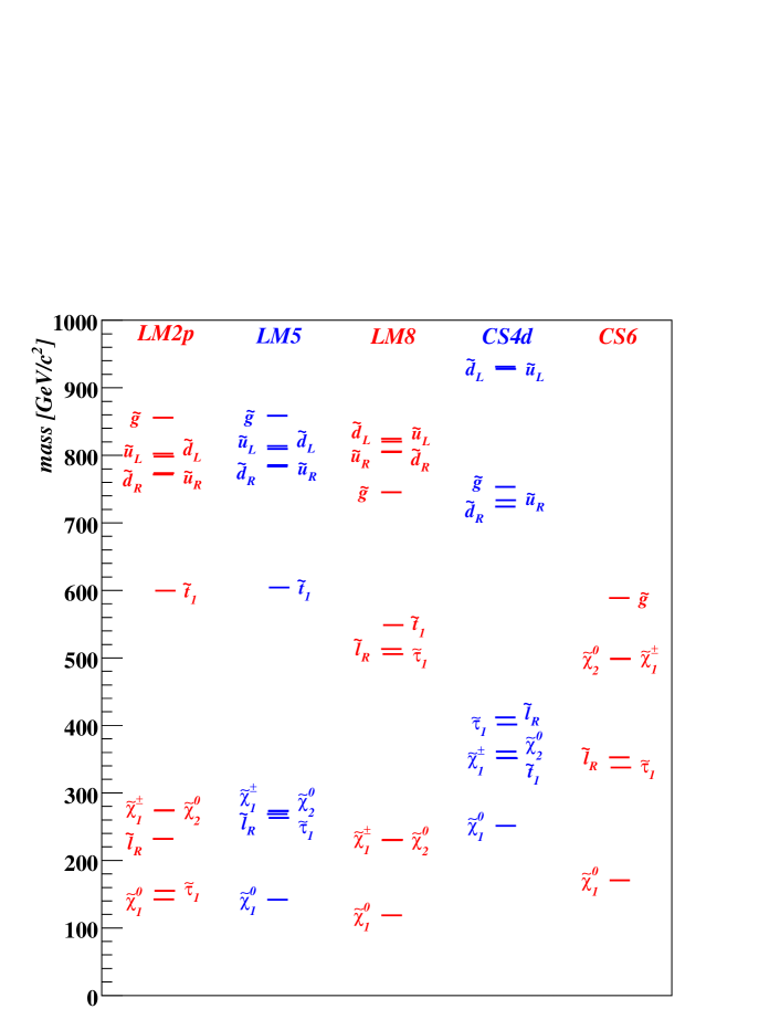
The five look-alike models of Group 1 are all MSSM models. Two of them (LM5 and LM8) are CMS SUSY benchmark models, while another (LM2p) is a slight variation of a CMS benchmark. It is a sobering coincidence that these are look-alikes of the $E_{T}^{\rm{miss}}$ analysis, since the benchmarks were developed by CMS to cover different experimental signatures, not produce look-alikes. To round out Group 1 we found two other MSSM look-alikes whose spectra and decay chains are as different from each other and from the three CMS benchmarks as we could make them.

The models are consistent with all current experimental constraints, but do not all give the “correct” relic density of dark matter. Any comparison of relic densities to the so-called WMAP constraints assumes at least three facts not yet in evidence: (i) that dark matter is a thermal relic, (ii) that there is only one significant species of dark matter and (iii) that cosmological evolution was entirely radiation-dominated from the time of dark matter decoupling until the time of Big Bang nucleosynthesis. A missing energy discovery at the LHC will help us test whether these assumptions have any validity. For example, model LM8 produces a relic density an order of magnitude larger than the WMAP upper bound; thus discriminating LM8 as a more likely explanation of an early missing energy discovery would call into question Gelmini:2006pq ; Barenboim:2006jh assumptions (i) and (iii), or could be a hint that the lightest neutralino is not absolutely stable.

LM2p, LM5 and LM8 are minimal supergravity models Chamseddine:1982jx -Hall:1983iz . They are specified by the usual high scale mSUGRA input parameters as shown in Table 4; because the resulting superpartner spectra depend strongly on RGE running from the high scale, a complete specification of the models also requires fixing the top quark mass and the particular spectrum generator program used. We have used $m_{\rm top}$ = 175 GeV and the ISAJET v7.69 generator isajet , in order to maintain compatibility with the CMS Physics TDR Ball:2007zza . Models LM5 and LM8 are then identical to the mSUGRA benchmark models of the CMS Physics TDR, while LM2p is almost identical to benchmark model LM2; LM2p has a slightly larger value of $m_{1/2}$ (360 versus 350 GeV) than LM2, which makes it more of a look-alike of the other Group 1 models.

Table 4: Input parameters for the mSUGRA models LM2p, LM5 and LM8. The notation comforms to isajet . The mass parameters and trilinear $A_{0}$ parameter have units of GeV.

	LM2p	LM5	LM8
$m_{0}$	185	230	500
$m_{1/2}$	360	360	300
$A_{0}$	0	0	-300
tan$\,\beta$	35	10	10
sign($\mu$)	+	+	+

Table 5: Input parameters for the MSSM models CS4d and CS6. The notation conforms to Djouadi:2006bz ; Djouadi:2002ze . The mass parameters and trilinear $A$ parameters have units of GeV.

	CS4d	CS6
$M_{1}$	620	400
$M_{2}$	930	600
$M_{3}$	310	200
$A_{\tau},A_{t},A_{b},A_{e},A_{u},A_{d}$	-400	-300
$M_{Q_{L}},M_{t_{R}},M_{b_{R}}$	340	2000
$M_{q_{u}},M_{u_{R}},M_{d_{R}}$	340	2000
$M_{\tau_{L}},M_{\tau_{R}},M_{e_{L}},M_{e_{R}}$	340	340
$M_{h_{u}}^{2},M_{h_{d}}^{2}$	115600	115600
tan$\,\beta$	10	10
sign($\mu$)	+	+

Table 6: Summary of LHC superpartner production for the Group 1 MSSM models LM2p, LM5, LM8, CS4d and CS6. The relative percentages are shown for each model, both before and after the event selection. The squark–squark percentages shown are excluding the contributions from pair production of the lightest stops, which are shown separately. Note that squark–chargino includes the production of either chargino, and squark-neutralino includes all of the four neutralinos. The category “other” includes weak production as well as the associated production of gluinos with charginos or neutralinos. The total NLO cross sections are from Prospino2 prospino2 .

	LM2p		LM5		LM8		CS4d		CS6
NLO cross section (pb)	8.6		8.1		12.7		14.5		12.6
	before	after	before	after	before	after	before	after	before	after
	cuts	cuts	cuts	cuts	cuts	cuts	cuts	cuts	cuts	cuts
squark–squark	33%	36%	32%	38%	22%	33%	19%	34%	0.1%	0.1%
squark–gluino	45%	55%	46%	52%	48%	54%	41%	55%	3.7%	7.4%
gluino–gluino	7.2%	6.4%	7.4%	6.4%	14%	8.3%	11%	8%	95%	92%
stop–stop	2.1%	1.1%	2.1%	0.9%	2.6%	1.5%	26%	1.4%	-	-
squark–chargino	2.1%	0.5%	2.1%	0.7%	1.4%	0.7%	0.2%	0.2%	-	-
squark–neutralino	1.7%	0.4%	1.8%	0.4%	1.2%	0.6%	0.6%	0.2%	-	-
other	9.5%	0.7%	9.3%	0.8%	11%	0.8%	1.9%	0.3%	1.1%	0.1%

The Group 1 models CS4d and CS6 are not minimal supergravity; they are more general high scale MSSM models based on the compressed supersymmetry idea of Martin Martin:2007gf ; Baer:2007uz . The high scale input parameters are shown in Table 5. We have used $m_{\rm top}$ = 175 GeV and the spectrum generator combination SuSpect v2.34 with SUSY-HIT v1.1 Djouadi:2002ze ; Djouadi:2006bz . Model CS4d is in fact part of the compressed SUSY model line defined in Martin:2007gf . Model CS6 is a modification of compressed SUSY where all of the squarks have been made very heavy, $\mathrel{\raisebox{-2.58334pt}{$\stackrel{{\scriptstyle\textstyle>}}{{\sim}}$}}2$ TeV.

The superpartner mass spectra of the Group 1 models are displayed in Figure 5. One notes immediately that all of the mSUGRA models are more similar to each other than they are to either of the more general MSSM models CS4d and CS6; this shows the limitations of the usual SUSY analyses that do not go beyond mSUGRA. As their name implies, the compressed SUSY models CS4d and CS6 have a compressed gaugino spectrum relative to mSUGRA; this produces either a light gluino (as in CS6) or a heavy LSP (as in CS4d).

The relative frequency of various LHC superpartner production processes is summarized in Table 6, for the Group 1 models both before and after our event selection. The production fractions are much more similar after the event selection than before it; this is expected because the selection shapes the kinematics of the surviving sample. Gluino pair production dominates for model CS6, while squark-gluino and squark-squark production dominate for the other four models. Pair production of the lightest stop is important for model CS4d before the selection cuts, but after the event selection very few of these events remain.

Table 7: Summary of most relevant superpartner decays for the MSSM models LM2p, LM5, LM8, CS4d and CS6.

	LM2p	LM5	LM8	CS4d	CS6
$\tilde{g}\rightarrow\tilde{q}q$	45%	45%	-	-	-
$\rightarrow\tilde{b}_{1}b$	25%	20%	14%	2%	-
$\rightarrow\tilde{t}_{1}t$	16%	23%	81%	94%	-
$\rightarrow q\bar{q}\tilde{\chi}_{1}^{0}$	-	-	5%	-	75%
$\tilde{u}_{L}\rightarrow d\tilde{\chi}_{1}^{\pm}$	64%	64%	55%	-	-
$\rightarrow u\tilde{\chi}_{2}^{0}$	32%	32%	27%	-	-
$\rightarrow u\tilde{g}$	-	-	-	83%	85%
$\tilde{u}_{R}\rightarrow u\tilde{\chi}_{1}^{0}$	99%	99%	62%	92%	-
$\rightarrow u\tilde{g}$	-	-	38%	-	85%
$\tilde{b}_{1}\rightarrow t\tilde{\chi}_{1}^{-}$	42%	36%	35%	20%	9%
$\rightarrow b\tilde{\chi}_{2}^{0}$	29%	23%	22%	14%	5%
$\rightarrow b\tilde{\chi}_{1}^{0}$	7%	2%	1%	50%	-
$\rightarrow b\tilde{g}$	-	-	-	-	85%
$\tilde{t}_{1}\rightarrow b\tilde{\chi}_{1}^{+}$	45%	43%	42%	-	-
$\rightarrow t\tilde{\chi}_{1}^{0}$	22%	25%	30%	-	4%
$\rightarrow t\tilde{g}$	-	-	-	-	96%
$\rightarrow bW^{+}\tilde{\chi}_{1}^{0}$	-	-	-	100%	-
$\tilde{\chi}_{1}^{\pm}\rightarrow W^{\pm}\tilde{\chi}_{1}^{0}$	5%	97%	100%	100%	2%
$\rightarrow\tilde{\tau}_{1}^{\pm}\nu_{\tau}$	95%	-	-	-	77%
$\tilde{\chi}_{2}^{0}\rightarrow Z\tilde{\chi}_{1}^{0}$	1%	11%	100%	100%	-
$\rightarrow h\tilde{\chi}_{1}^{0}$	3%	85%	-	-	2%
$\rightarrow\tilde{\tau}_{1}\tau$	96%	3%	-	-	77%
$\tilde{\tau}_{1}\rightarrow\tau\tilde{\chi}_{1}^{0}$	100%	100%	88%	98%	100%

Table 7 shows the most relevant superpartner decay branching fractions. For models LM2p and LM5, gluino decay is predominantly to quark$+$squark; for LM8 and CS4d it is dominantly to top and the lightest stop, and gluinos decay in CS6 mostly through the three-body mode $qq\tilde{\chi}_{1}^{0}$. For models LM2p, LM5 and LM8, left-squarks cascade through quark$+$chargino or quark$+$second neutralino; right-squarks have a two-body decay to quark$+$LSP; right-squarks in model LM8 also have a large branching to quark$+$gluino. In model CS4d left-squarks decay almost entirely to quark$+$gluino, while right-squarks decay almost entirely to quark$+$LSP; for CS6 all squarks except the stop decay dominantly to quark$+$gluino.

In models LM2p, LM5 and LM8 the decays of the lightest stop split between $b+$chargino and top$+$LSP; for CS4d $\tilde{t}_{1}$ decays 100% via the three-body mode $bW^{+}\tilde{\chi}_{1}^{0}$, while for CS6 almost all of the decays are to top$+$gluino.

Chargino decay is dominated by decays to the lightest stau and a neutrino for models LM2p and CS6, and by decays to $W+$LSP for models LM5, LM8 and CS4d. The second neutralino $\tilde{\chi}_{2}^{0}$ decays almost entirely to $\tau+$stau for models LM2p and CS6, and goes 100% to $Z+$LSP in models LM8 and CS4d. The LM5 model has the distinct feature that 85% of $\tilde{\chi}_{2}^{0}$ decays are to Higgs$+$LSP.

Table 8 shows the most significant inclusive final states for the Group 1 models. By final state we mean that all unstable superpartners have decayed, while Standard Model particles are left undecayed. We use $q$ to denote any first or second generation quark or antiquark, but list bottom and top quarks separately. The percentage frequency of each final state is with respect to the events passing our selection. The final states are inclusive, thus e.g. the events in the $qqq\;\tilde{\chi}_{1}^{0}\tilde{\chi}_{1}^{0}$ final state are a subset of those in the $qq\;\tilde{\chi}_{1}^{0}\tilde{\chi}_{1}^{0}$ final state, and the total percentages in each column exceed 100% . By the same token, most exclusive final states actually have more partons than are listed for the corresponding inclusive entries in Table 8, so even at leading order parton level they produce more jets.

For models LM2p, LM5 and CS6, the dominant inclusive final state is $qq\tilde{\chi}_{1}^{0}\tilde{\chi}_{1}^{0}+X$, i.e. multijets plus missing energy from the two LSPs. This is the motivation behind the design of our analysis. For model CS4d, the most likely production is squark-gluino followed by squark decay to quark$+$LSP; the gluino then decays to top$+$stop, with the stop decaying via the three-body mode $bW^{+}\tilde{\chi}_{1}^{0}$. The most popular exclusive final state is thus $btWq\tilde{\chi}_{1}^{0}\tilde{\chi}_{1}^{0}$. Similarly, for LM8 the most popular exclusive final states are $btWq\tilde{\chi}_{1}^{0}\tilde{\chi}_{1}^{0}$ and $ttq\tilde{\chi}_{1}^{0}\tilde{\chi}_{1}^{0}$, from squark-gluino production followed by gluino decay to top$+$stop.

Final states with $W$’s are prevalent in models LM5, LM8 and CS4d. The LM2p model stands out because of the high probability of taus in the final state. Model LM5 produces a significant number of light Higgses from superpartner decays. Model LM8 has a large fraction of events with $Z$ bosons in the final state. Model CS4d is enriched in final states with multiple tops and $W$’s, of which one representative example is shown: $bbttWW\tilde{\chi}_{1}^{0}\;\tilde{\chi}_{1}^{0}$.

Table 8: Summary of significant inclusive partonic final states for the Group 1 MSSM models LM2p, LM5, LM8, CS4d and CS6. By final state we mean that all unstable superpartners have decayed, while Standard Model particles are left undecayed. Here $q$ denotes any first or second generation quark or antiquark, and more generally the notation does not distinguish particles from antiparticles. The percentage frequency of each final state is with respect to the events passing our selection.The final states are inclusive, thus e.g. the events in the $qqq\;\tilde{\chi}_{1}^{0}\tilde{\chi}_{1}^{0}$ final state are a subset of those in the $qq\;\tilde{\chi}_{1}^{0}\tilde{\chi}_{1}^{0}$ final state, and the total percentages in each column exceed 100% .

	LM2p	LM5	LM8	CS4d	CS6
$qq\;\tilde{\chi}_{1}^{0}\;\tilde{\chi}_{1}^{0}$	57%	61%	34%	38%	98%
$qqq\;\tilde{\chi}_{1}^{0}\;\tilde{\chi}_{1}^{0}$	20%	19%	3%	4%	79%
$qqqq\;\tilde{\chi}_{1}^{0}\;\tilde{\chi}_{1}^{0}$	1%	1%	1%	1%	77%
$\tau\;\nu_{\tau}\;q\;\tilde{\chi}_{1}^{0}\;\tilde{\chi}_{1}^{0}$	39%	1%	-	-	1%
$\tau\tau\;q\;\tilde{\chi}_{1}^{0}\;\tilde{\chi}_{1}^{0}$	25%	1%	-	-	1%
$b\;q\;\tilde{\chi}_{1}^{0}\;\tilde{\chi}_{1}^{0}$	30%	25%	33%	69%	19%
$b\;t\;W\;q\;\tilde{\chi}_{1}^{0}\;\tilde{\chi}_{1}^{0}$	10%	19%	31%	67%	-
$W\;q\;\tilde{\chi}_{1}^{0}\;\tilde{\chi}_{1}^{0}$	25%	52%	56%	93%	-
$h\;q\;\tilde{\chi}_{1}^{0}\;\tilde{\chi}_{1}^{0}$	3%	20%	-	-	-
$tt\;q\;\tilde{\chi}_{1}^{0}\;\tilde{\chi}_{1}^{0}$	9%	4%	40%	11%	2%
$Z\;q\;\tilde{\chi}_{1}^{0}\;\tilde{\chi}_{1}^{0}$	10%	8%	35%	11%	-
$Z\;W\;q\;\tilde{\chi}_{1}^{0}\;\tilde{\chi}_{1}^{0}$	2%	6%	23%	6%	-
$bb\;tt\;WW\;\tilde{\chi}_{1}^{0}\;\tilde{\chi}_{1}^{0}$	-	-	2%	18%	-

Table 9: Estimated number of events passing our selection per 100 pb^-1 of integrated luminosity, for the Group 1 models LM2p, LM5, LM8, CS4d and CS6. These estimates use NLO cross sections and the CTEQ5L pdfs.

LM2p	LM5	LM8	CS4d	CS6
211	200	195	195	212

Summarizing this discussion, we list the most significant features of each model in Group 1:

Model LM2p: 800 GeV squarks are slightly lighter than the gluino, and there is a 155 GeV stau. Dominant production is squark-gluino and squark-squark. Left-squarks decay about two-thirds of the time to quark$+$chargino, and one-third to quark$+$LSP; right-squarks decay to quark$+$LSP. Gluino decay is mostly to quark$+$squark. Charginos decay to the light stau plus a neutrino, while the second neutralino decays to $\tau+$stau. Two-thirds of the final states after event selection have at least one $\tau$.

Model LM5: 800 GeV squarks are slightly lighter than the gluino. Dominant production is squark-gluino and squark pairs. Left-squark decays about two-thirds to quark$+$chargino, and one-third to quark$+$LSP; right-squarks decay to quark$+$LSP. Gluino decay is mostly to quark$+$squark. Charginos decay to a $W$ and an LSP, while the second neutralino decays to a light Higgs and an LSP. After selection more than half of final states have a $W$ boson, and a fifth have a Higgs.

Model LM8: The 745 GeV gluino is slightly lighter than all of the squarks except $\tilde{b}_{1}$ and $\tilde{t}_{1}$. Dominant production is squark-gluino and squark pairs. Left-squarks decay about two-thirds to quark$+$chargino, and one-third to quark$+$LSP; right-squarks decay two-thirds to quark$+$LSP and one-third to quark$+$gluino. Gluino decay is dominantly to top and a stop; the 548 GeV stops decay mostly to $b+$chargino or top$+$LSP. Charginos decay to $W+$LSP, and the second neutralino decays to $Z+$LSP. After selection 40% of final states have two tops, which may or may not have the same sign. More than half of the final states have a $W$, more than a third have a $Z$, and a quarter have both a $W$ and a $Z$.

Model CS4d: The 753 GeV gluino is in between the right-squark and left-squark masses. The LSP is relatively heavy, 251 GeV, and the ratio of the gluino to LSP mass is small compared to mSUGRA models. Dominant production is squark-gluino and squark-squark. Left-squarks decay to quark$+$gluino, and right-squarks decay to quark$+$LSP. Gluinos decay to top and a stop; the 352 GeV stops decay 100% to $bW^{+}\tilde{\chi}_{1}^{0}$. Two-thirds of the final states contain $btWq\tilde{\chi}_{1}^{0}\tilde{\chi}_{1}^{0}$, and a significant fraction of these contain more $b$’s, $t$’s and $W$’s.

Model CS6: The 589 GeV gluino is much lighter than the 2 TeV squarks, and the ratio of the gluino to LSP mass is small compared to mSUGRA models. Production is 92% gluino-gluino, and gluinos decay predominantly via the three-body mode $qq\tilde{\chi}_{1}^{0}$. The final states consist almost entirely of three or four quarks plus two LSPs, with a proportionate amount of the final state quarks being $b$’s.

Figure 6: The mass spectra of the models LH2, NM6, NM4 and CS7. Only the most relevant partners are shown: the lighter gauginos $\tilde{\chi}_{1}^{0}$, $\tilde{\chi}_{2}^{0}$ and $\tilde{\chi}_{1}^{\pm}$, the lightest stau $\tilde{\tau}_{1}$, the right-smuon and selectron denoted collectively as $\tilde{\ell}_{R}$, the gluino, and the left/right up and down squarks $\tilde{u}_{L}$, $\tilde{u}_{R}$, $\tilde{d}_{L}$ and $\tilde{d}_{R}$. For the little Higgs model LH2, the relevant quark and vector partners are shown: the gauge boson partners $A_{H}$, $Z_{H}$, $W_{H}$, and the three generations of quark partners $u^{i}_{H}$, $d^{i}_{H}$, $i=1,2,3$.

Table 10: Parameter choices defining the little Higgs model LH2. We choose our conventions to agree with those found in Hubisz:2005tx : $f$ is the symmetry-breaking scale, $\kappa_{q}^{i}$ is the $T$-odd quark Yukawa coupling, $\kappa_{l}^{i}$ is the $T$-odd lepton Yukawa coupling and $\sin\alpha$ is a mixing angle. CKM mixing has been suppressed for our analysis.

. $f$ 700 GeV $\kappa_{q}^{i}$ 0.55 $\kappa_{l}^{i}$ 2.0 $\sin\alpha$ 0.17

Table 11: Input parameters for the MSSM models NM6, NM4 and CS7. The notation conforms to Djouadi:2006bz ; Djouadi:2002ze . The mass parameters and trilinear $A$ parameters have units of GeV.

	NM6	NM4	CS7
$M_{1}$	138	105	428
$M_{2}$	735	466	642
$M_{3}$	2082	1600	214
$A_{t}$	0	-50	-321
$A_{b}$	4000	0	-321
$A_{\tau},A_{t},A_{b},A_{e},A_{u},A_{d}$	0	0	-321
$M_{Q_{L}}$	755	590	2000
$M_{t_{R}}$	760	580	2000
$M_{q_{u}}$	770	590	2000
$M_{u_{R}},M_{b_{R}}$	770	580	2000
$M_{d_{R}}$	765	580	2000
$M_{\tau_{L}},M_{\tau_{R}},M_{e_{L}},M_{e_{R}}$	2500	540	340
$M_{h_{u}}^{2},M_{h_{d}}^{2}$	115600	115600	115600
tan$\,\beta$	10	10	10
sign($\mu$)	+	+	+

IV.2 Group 2

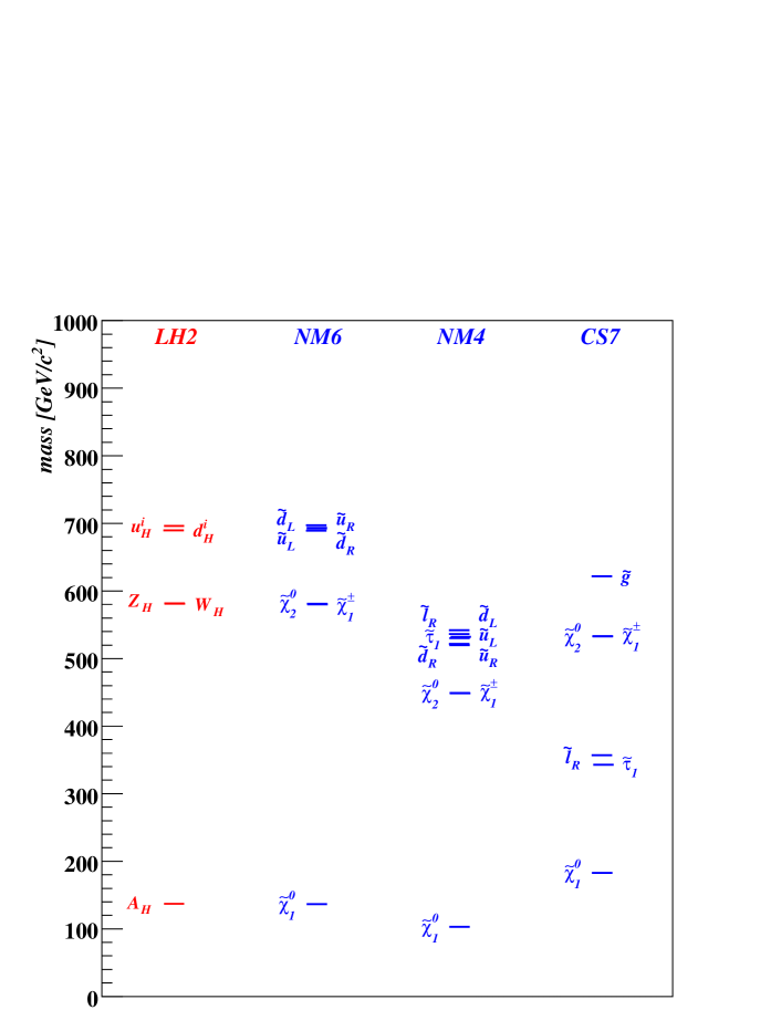
Group 2 consists of three look-alike models: LH2, NM4 and CS7, and a comparison model NM6. LH2 is a littlest Higgs model with conserved $T$ parity. The parameter choices defining this model are shown in Table 10. The mass spectrum of the lighter partners is shown in Figure 6; not shown are the heavier top partners $T_{+}$, $T_{-}$ with tuned masses 3083 and 3169 GeV respectively, the charged lepton partners $\ell^{1}_{H}$, $\ell^{2}_{H}$, $\ell^{3}_{H}$ with mass 2522 GeV and the neutrino partners $\nu^{1}_{H}$, $\nu^{2}_{H}$, $\nu^{3}_{H}$ with mass 2546 GeV. Model LH2 is consistent with all current experimental constraints Hubisz:2005tx ; Asano:2006nr .

NM6, NM4 and CS7 are all MSSM models. The high scale input parameters are listed in Table 11. We have used $m_{\rm top}$ = 175 GeV and the spectrum generator SuSpect v2.34. The mass spectra are shown in Figure 6; not shown are the heavy gluinos of NM6 and NM4 with masses 2000 and 1536 GeV respectively, and the $\mathrel{\raisebox{-2.58334pt}{$\stackrel{{\scriptstyle\textstyle>}}{{\sim}}$}}2$ TeV squarks of model CS7.

The SUSY model NM6 was chosen to have a spectrum identical to that of the little Higgs model LH2, apart from the heavy gluino that has no counterpart in LH2. Thus to a good approximation these two models differ only by the spins of the partners. While LH2 and NM6 are in this sense twins, they are not look-alikes of our benchmark inclusive missing energy analysis. Models NM4 and CS7, by contrast, are SUSY look-alikes of the little Higgs model LH2. The superpartner spectrum of NM4 is roughly similar to the partner spectrum of LH2, but the superpartners are lighter. The spectrum of CS7 has no similarity to that of LH2.

The relative frequency of various LHC little Higgs partner production processes are shown in Table 12, for the LH2 model both before and after our event selection. For LH2 the predominant process is $gg$ or $q\bar{q}$ partons initiating QCD production of a heavy partner quark-antiquark pair; this process is completely equivalent to $t\bar{t}$ production at the LHC. The most striking feature of Table 12 is that nearly half of the total production involves weak interactions. For example the second largest production mechanism, 14% of the total, has two valence quarks in the initial state producing a pair of first generation heavy partner quarks; at tree-level this is from $s$-channel annihilation into a $W$ and $t$-channel exchange of a $Z_{H}$ or $A_{H}$ partner.

The superpartner production at the LHC for the SUSY models NM6, NM4 and CS7 is summarized in Table 13. For NM6 and NM4 a major contribution is from $gg$ or $q\bar{q}$ partons initiating QCD production of a squark-antisquark pair. Production of a first generation squark pair from two initial state valence quarks is also important; in contrast to the LH2 non-SUSY analog this is a QCD process with $t$-channel exchange of the heavy gluino. For model CS7, which has a light gluino and very heavy squarks, 96% of the production is gluino pairs.

The primary decay modes for the lighter LH2 partners are shown in Table 14, while those for the SUSY models are summarized in Table 15. Tables 16 and 17 display the most significant inclusive partonic final states for the Group 2 models.

For LH2, a large fraction of heavy partner quarks have a direct 2-body decay to a quark and an $A_{H}$ WIMP. The other heavy partner quark decay mode is a two stage cascade decay via the $W_{H}$ and $Z_{H}$ partner bosons. Since the $W_{H}$ decays 100% to $WA_{H}$ while the $Z_{H}$ decays 100% to $hA_{H}$, a large fraction of events have a $W$ or a Higgs in the final state.

Analogous statements apply to the SUSY models NM6 and NM4. We see that 100% of right-squarks and a significant fraction of left-squarks undergo a direct 2-body decay to quark$+$LSP. The rest have mostly a two stage cascade via the lightest chargino $\tilde{\chi}_{1}^{\pm}$ or the second neutralino $\tilde{\chi}_{2}^{0}$. Since $\tilde{\chi}_{1}^{\pm}$ decays 100% to $W+$LSP, while the $\tilde{\chi}_{2}^{0}$ decays dominantly to a Higgs$+$LSP, a significant fraction of events have a $W$ or a Higgs in the final state.

For the remaining SUSY model CS7, gluino pair production is followed by 3-body decays of each gluino to a quark-antiquark pair + LSP. As can be seen in Table 17, this leads to high jet multiplicity but nothing else of note besides a proportionate number of $b\bar{b}$ and $t\bar{t}$ pairs.

Table 12: Production channels for little Higgs partners in the LH2 model, both before and after the event selection. Here $Q$ stands for any of the quark partners $u^{i}_{H}$, $d^{i}_{H}$, $i=1,2,3$. The total LO cross section as reported by MadEvent is 6.5 pb.

	before cuts	after cuts
$Q_{i}\bar{Q}_{i}$	55%	64%
$u^{i}_{H}d^{i}_{H}$, $u^{i}_{H}u^{i}_{H}$, $d^{i}_{H}d^{i}_{H}$	14%	16%
$d^{i}_{H}W^{+}_{H}$, $u^{i}_{H}W^{-}_{H}$	12%	7%
$u^{i}_{H}Z_{H}$, $u^{i}_{H}A_{H}$, $d^{i}_{H}Z_{H}$, $d^{i}_{H}A_{H}$	9%	5%
$Q_{i}\bar{Q}_{j}$, $i\neq j$	3%	3%
other	7%	5%

Table 13: Summary of LHC superpartner production for the Group 2 MSSM models NM6, NM4 and CS7. The relative percentages are shown for each model, both before and after the event selection. Here $\tilde{q}_{i}$ denotes any of the three generations of left and right squarks. Note that squark–chargino includes the production of either chargino, and squark-neutralino includes all of the four neutralinos. The LO total cross sections are as reported by MadEvent.

	NM6		NM4		CS7
LO cross section (pb)	2.3		10.3		5.0
	before	after	before	after	before	after
	cuts	cuts	cuts	cuts	cuts	cuts
$\tilde{q}_{i}\bar{\tilde{q}}_{i}$	31%	29%	34%	26%	-	-
$\tilde{u}\tilde{d}$, $\tilde{u}\tilde{u}$, $\tilde{d}\tilde{d}$	32%	28%	29	23%	-	-
squark–gluino	3%	10%	5%	23%	4%	8%
gluino–gluino	-	-	-	-	96%	91%
squark–chargino	2%	2%	3%	1%	-	-
squark–neutralino	4%	1%	4%	-	-	-
$\tilde{q}_{i}\bar{\tilde{q}}_{j}$, $i\neq j$	15%	17%	17%	14%	-	-
other	13%	13%	8%	13%	-	-

Table 14: Decay modes for the lighter little Higgs partners of model LH2.

$d^{i}_{H}$, $i=1,2$	$\rightarrow u^{i}W_{H}$	52%
	$\rightarrow d^{i}Z_{H}$	26%
	$\rightarrow d^{i}A_{H}$	22%
$d^{3}_{H}$	$\rightarrow bZ_{H}$	54%
	$\rightarrow bA_{H}$	46%
$u^{i}_{H}$, $i=1,2$	$\rightarrow d^{i}W_{H}$	31%
	$\rightarrow u^{i}Z_{H}$	15%
	$\rightarrow u^{i}A_{H}$	54%
$u^{3}_{H}$	$\rightarrow bW_{H}$	41%
	$\rightarrow tA_{H}$	59%
$W_{H}$	$\rightarrow WA_{H}$	100%
$Z_{H}$	$\rightarrow hA_{H}$	100%

Table 15: Summary of most relevant superpartner decays for the MSSM models NM6, NM4 and CS7.

	NM6	NM4	CS7
$\tilde{g}\rightarrow\tilde{q}q$	66%	67%	-
$\rightarrow\tilde{b}b$	17%	17%	-
$\rightarrow\tilde{t}_{1}t$	17%	16%	-
$\rightarrow q\bar{q}\tilde{\chi}_{1}^{0}$	-	-	99%
$\tilde{u}_{L}\rightarrow d\tilde{\chi}_{1}^{\pm}$	39%	59%	12%
$\rightarrow u\tilde{\chi}_{1}^{0}$	44%	12%	-
$\tilde{u}_{R}\rightarrow u\tilde{\chi}_{1}^{0}$	100%	100%	4%
$\tilde{b}_{1}\rightarrow b\tilde{\chi}_{2}^{0}$	24%	14%	6%
$\rightarrow b\tilde{\chi}_{1}^{0}$	70%	86%	-
$\tilde{t}_{1}\rightarrow b\tilde{\chi}_{1}^{+}$	40%	27%	-
$\rightarrow t\tilde{\chi}_{1}^{0}$	60%	73%	5%
$\tilde{\chi}_{1}^{\pm}\rightarrow W^{\pm}\tilde{\chi}_{1}^{0}$	100%	100%	1%
$\rightarrow\tilde{\tau}\nu_{\tau}$	-	-	35%
$\rightarrow\tilde{\nu}\ell$	-	-	28%
$\rightarrow\tilde{\nu}\tau$	-	-	17%
$\tilde{\chi}_{2}^{0}\rightarrow Z\tilde{\chi}_{1}^{0}$	22%	19%	-
$\rightarrow h\tilde{\chi}_{1}^{0}$	78%	81%	-
$\rightarrow\tilde{\tau}\tau$	-	-	39%
$\rightarrow\tilde{\nu}\nu$	-	-	45%
$\rightarrow\tilde{\ell}\ell$	-	-	16%

Table 16: Significant inclusive partonic final states for the little Higgs model LH2. The percentage frequency of each final state is with respect to the events passing our selection.

$qq\;A_{H}A_{H}$	64%
$W\;qq\;A_{H}A_{H}$	39%
$h\;qq\;A_{H}A_{H}$	22%
$bb\;A_{H}A_{H}$	14%
$WW\;qq\;A_{H}A_{H}$	8%
$hh\;bb\;A_{H}A_{H}$	4%
$hh\;qq\;A_{H}A_{H}$	3%
$tt\;A_{H}A_{H}$	3%

Table 17: Significant inclusive partonic final states for the Group 2 MSSM models NM6, NM4 and CS7. The percentage frequency of each final state is with respect to the events passing our selection.

	NM6	NM4	CS7
$qq\;\tilde{\chi}_{1}^{0}\;\tilde{\chi}_{1}^{0}$	84%	83%	100%
$qqq\;\tilde{\chi}_{1}^{0}\;\tilde{\chi}_{1}^{0}$	8%	16%	100%
$qqqq\;\tilde{\chi}_{1}^{0}\;\tilde{\chi}_{1}^{0}$	-	-	95%
$bb\;q\;\tilde{\chi}_{1}^{0}\;\tilde{\chi}_{1}^{0}$	2%	5%	11%
$W\;qq\;\tilde{\chi}_{1}^{0}\;\tilde{\chi}_{1}^{0}$	26%	35%	-
$h\;q\;\tilde{\chi}_{1}^{0}\;\tilde{\chi}_{1}^{0}$	14%	19%	-
$tt\;q\;\tilde{\chi}_{1}^{0}\;\tilde{\chi}_{1}^{0}$	1%	1%	11%
$Z\;q\;\tilde{\chi}_{1}^{0}\;\tilde{\chi}_{1}^{0}$	4%	5%	-
$WW\;q\;\tilde{\chi}_{1}^{0}\;\tilde{\chi}_{1}^{0}$	4%	9%	-

Table 18: Estimated number of events passing our selection per 100 pb^-1 of integrated luminosity, for the Group 2 models LH2, NM6, NM4 and CS7. These estimates use leading order cross sections and the CTEQ5L pdfs.

LH2	NM6	NM4	CS7
94	43	97	91

IV.3 Comparison of models differing only by spin

We have already noted that SUSY model NM6 has a superpartner spectrum almost identical to the heavy partner spectrum of the non-SUSY little Higgs model LH2. The only relevant difference, other than the spins of the partners, is that model NM6 has a very heavy 2 TeV gluino that has no analog in LH2. Despite being very heavy, the gluino does make a significant contribution to squark-squark production via $t$-channel exchange.

This pair of models provides the opportunity for a comparison of realistic models that within a good approximation differ only by the spins of the partner particles. If it turned out that these two models were look-alikes in our benchmark inclusive missing energy analysis, then discriminating them would be physically equivalent to determining the spins of at least some of the heavy partners.

It is an ancient observation (see e.g. Farrar:1980uy ) that models differing only by the spins of the new heavy exotics have significant differences in total cross section. The most familiar example is the comparison of pair production of heavy leptons near threshold with pair production of spinless sleptons. For mass $m$ and total energy $\sqrt{s}$, the lepton cross section is proportional to $\beta$,

$$\textstyle{\beta\equiv\sqrt{1-\frac{4m^{2}}{s}}}\;,$$ (2)

while the slepton cross section is proportional to $\beta^{3}$. Thus slepton production is suppressed near threshold compared to production of heavy leptons with the same mass. A somewhat less familiar fact is that the sleptons never catch up: even if we introduce both left and right sleptons, to match the degrees of freedom of a Dirac lepton, the total cross section for left+right slepton pairs is one-half that of Dirac lepton pairs in the high energy limit $\beta\rightarrow 1$.

For the hadroproduction relevant to our models LH2 and NM6, the discussion is more complicated: the most relevant details and references are presented in our Appendix. From Tables 12 and 13, we see a large difference in the leading order total LHC cross sections for these models: 6.5 pb for LH2 versus only 2.3 pb for NM6. Thus the non-SUSY twin has almost a factor of three cross section enhancement, in spite of the fact that the SUSY model benefits from some extra production mediated by gluinos.

The possibility of distinguishing SUSY from non-SUSY twins at the LHC using total cross section was first suggested by Datta, Kane and Toharia Datta:2005vx , and studied in more detail in Kane:2008kw . To implement this idea, we must also compare the relative efficiencies of the SUSY and non-SUSY twins in a real analysis, since what is measured in an experiment is not total cross section but rather cross section times efficiency.

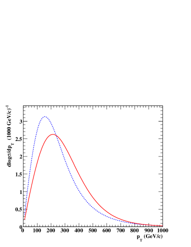
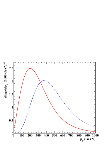
An important observation is that the $p_{T}$ distributions, in addition to the total cross sections, have large differences due solely to differences in spin. As an example, consider the LHC production of a pair of 500 GeV heavy quarks, versus the production of a pair of 500 GeV squarks. We can compare the $p_{T}$ distributions by computing

$$\frac{d{\rm log}\,\sigma}{dp_{T}}=\frac{1}{\sigma}\frac{d\sigma}{dp_{T}}\,$$ (3)

where we factor out the difference in the total cross sections. Using the analytic formulae reviewed in the Appendix, we have computed (3) for two relevant partonic subprocesses. The first is gluon-gluon initiated production, for which the fully differential cross sections are given in (42) and (43); at leading order this arises from an $s$-channel annihilation diagram, a gluon seagull for the squark case, and $t$ and $u$ channel exchanges of either the spin 1/2 heavy quark or the spin 0 squark. The second example is quark-antiquark initiated production, in the simplest case where the quark flavor does not match the quark/squark partner flavor; at leading order there is only one diagram: $s$-channel annihilation. The fully differential cross sections are given in (28) and (29).

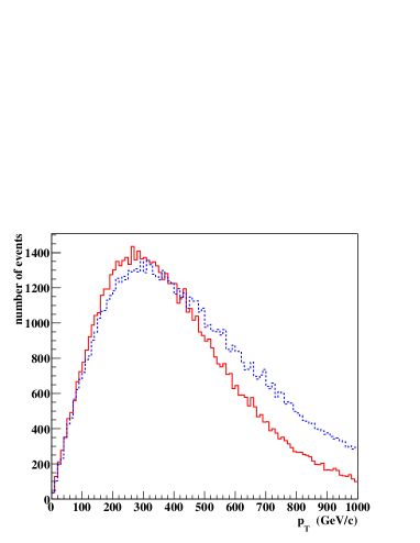
For this simple example, we have integrated the fully differential cross sections over the parton fluxes, using the CTEQ5L parton distribution functions. The resulting normalized $p_{T}$ distributions are shown in Figures 7 and 8. For the $gg$ initiated production the SUSY case has a significantly softer $p_{T}$ distribution, while for the $q\bar{q}$ initiated production the SUSY case has a significantly harder $p_{T}$ distribution.

We see similar differences in the complete models LH2 and NM6. Figure 9 shows a comparison of the $p_{T}$ distributions for heavy quark partner production from LH2 and squark production for NM6. All of the leading order partonic subprocesses are combined in the plot, and no event selection has been performed. The $p_{T}$ distribution for the SUSY model is harder than for the non-SUSY model. Part of this net effect is due to intrinsic spin differences e.g. as depicted in Figure 8, and part is due to SUSY diagrams with virtual gluino exchange. One would expect SUSY events to have a higher efficiency to pass our missing energy selection than non-SUSY events. Indeed this is the case: 19% of NM6 events overall pass the selection, whereas only 14% of LH2 events do. The higher efficiency of SUSY NM6 events in passing the selection somewhat compensates for the smaller total cross section compared to the non-SUSY LH2.

The event counts can be obtained by multiplying each total cross section times the total efficiency times the integrated luminosity. For a 100 pb^-1 sample, the total signal count is 94 events for model LH2 and 43 events for model NM6. The net result is that although LH2 and NM6 are twins in the sense of their spectra, they are not missing energy look-alikes in our benchmark analysis. Thus the good news is that, for models that differ only (or almost only) by spin, the event count in the discovery data sample is already good enough to discriminate them. This is one of the important conclusions of our study.

However this is also something of an academic exercise, since in the real experiment we will need to discriminate a large class of SUSY models from a large class of non-SUSY models. In this comparison a SUSY model can be a look-alike of a non-SUSY model even though the spectra of partner particles don’t match. This is what happens with SUSY models NM4 and CS7, which are both look-alikes of LH2. Model NM4 looks particularly challenging, since its superpartner spectrum is basically just a lighter version of NM6. Compared to NM6, the total cross section of NM4 is more than 4 times larger (10.3 pb) while the efficiency to pass our missing energy selection is only half as good (9%). This gives a total count of 97 events for 100 pb^-1, making NM4 a look-alike of LH2.

Figure 7: Comparison of the normalized $p_{T}$ distributions for leading order $gg$ initiated production of a pair of 500 GeV particles. The solid (red) line corresponds to quark-antiquark pair; the dot-dashed (blue) line to a squark-antisquark pair. The distributions have been integrated over the parton fluxes using the CTEQ5L pdfs.

Figure 8: Comparison of the normalized $p_{T}$ distributions for leading order $q\bar{q}$ initiated production of a pair of 500 GeV particles, for the case that the initial parton flavor does not match the final parton flavor. The solid (red) line corresponds to quark-antiquark pair; the dot-dashed (blue) line to a squark-antisquark pair. The distributions have been integrated over the parton fluxes using the CTEQ5L pdfs.

Figure 9: Comparison of the $p_{T}$ distributions for heavy quarks from the little Higgs model LH2 and squarks from the “twin” SUSY model NM6. The solid (red) line corresponds to heavy quark partners from model LH2; the dashed (blue) line to squarks from model NM6. For both models 100,000 events were generated using MadGraph and the CTEQ5L pdfs; no selection was applied.

V Observables

Having in mind an early discovery at the LHC, e.g. in the first $100$ pb^-1 of understood data, we have made conservative assumptions about the physics objects that will be sufficiently well-understood for use in our look-alike analysis of a missing energy discovery.

We assume that we can reconstruct and count high $E_{T}$ jets and hard tracks, as is required for our benchmark missing energy selection. We do not assume that validated jet corrections for multijet topologies will be available. We assume it will be possible to use the uncorrected (raw) $E_{T}^{\rm{miss}}$(without subtracting the momentum of muons or correcting for other calorimetric effects).

We assume the ability to reconstruct and count high $p_{T}$ muons; a study of $Z\rightarrow\mu^{+}\mu^{-}$ events is a necessary precursor to understanding the Standard Model $E_{T}^{\rm{miss}}$ backgrounds. It will also be possible to count high $E_{T}$ electrons, however we are not yet including electrons in our study because of the high “fake” rate expected at start-up. Multiflavor multilepton signatures are of great importance as model discriminators, though challenging with small data sets; this is worthy of a separate dedicated study Moortgat-Pape ; Baer:2008kc .

In our study instead of applying sophisticated $b$ and $\tau$ tagging algorithms we isolate enriched samples of $b$ quarks and hadronic $\tau$’s, by defining simple variables similar to the typical components of the complete tagging algorithms: leptons in jets, track counting, and impact parameter of charged tracks, to mention a few. This “poor man’s” tagging is not sufficient to obtain pure samples of $b$’s or $\tau$’s, but allows the discrimination of look-alike models with large differences in the $b$ or $\tau$ multiplicity.

V.1 Inclusive counts and ratios

We build our look-alike analysis strategy using simple ingredients. We start with the four trigger boxes defined in section II.2: MET, DiJet, TriJet and Muon20. For the simulated data samples corresponding to each box, we compute the following inclusive counts of jets and muons:

• N, the number of events in a given box after our benchmark selection.

• N(nj), the number of events with at least n jets (n=3,4,5). Note that N(3j) = N because of our selection.

• N(m$\mu$-nj), the number of events with at least n jets and m muons (n=3,4 and m=1,2).

• N(ss$\mu$), the number of events with at least two same-sign muons.

• N(os$\mu$), the number of events with at least two opposite-sign muons.

In these counts a muon implies a reconstructed muon with $p_{T}>20$ GeV/$c$ and $|\eta|<2.4$ with no isolation requirement.

From these inclusive counts we can define various interesting ratios. All of the ratios are of correlated observables. Examples of ratios are:

• r(nj)(3j)$\equiv$N(nj)/N(3j), with n=4,5, a measure of jet multiplicity.

• r(2$\mu$-nj)(1$\mu$-nj)$\equiv$N(2$\mu$-nj)/N(1$\mu$-nj), with n=3,4, a measure of muon multiplicity.

In appropriately chosen ratios of inclusive counts, important systematic effects cancel partially or completely. For example, if the detector simulation does not precisely reproduce the $E_{T}$ spectrum of signal jets as seen in the real detector, this introduces a systematic error in the N(nj) counts, since jets are only counted if they have $E_{T}$$>30$ GeV. However we expect partial cancellation of this in the ratio of inclusive counts r(4j)(3j). Another large systematic in the jet counts, the pdf uncertainty, also cancels partially in the ratios. The luminosity uncertainty cancels completely in the jet ratios. As we discuss below, ratios of correlated observables are also less sensitive to statistical fluctuations.

In order to enhance the robustness and realism of our study, we have cast all of our physical observables into the form of inclusive counts and ratios thereof, and our look-alike analysis only uses the ratios. This has the added advantage of allowing us to compare different discriminating variables on a more even footing. In the next five subsections we explain how this casting into counts and ratios is done.

V.2 Kinematic observables

As noted in Section II, the distribution of the missing transverse energy in the signal events is related to $m_{\rm dm}$, the mass of the WIMP, as well as to $m_{\rm p}$, the mass of the parent particles produced in the original $2\rightarrow 2$ partonic subprocess. In the benchmark $E_{T}^{\rm{miss}}$ selection, we used the kinematic variable $H_{T}$, as well as the $E_{T}$ of the leading and second leading jets. The distributions of these kinematic variables are also related to the underlying mass spectrum of the heavy partners.

We have employed two other kinematic variables in our study. The first is $M$, the total invariant mass of all of the reconstructed jets and muons in the event. The second is $M_{\rm eff}$, the scalar sum of the $E_{T}^{\rm{miss}}$ with the $E_{T}$ of all the jets in the event.

Figures 10-13 show a comparison of the $M_{\rm eff}$, $H_{T}$, $M$ and $E_{T}^{\rm{miss}}$ distributions, after selection, for models LM2p, CS4d and CS6. These models, though look-alikes of our $E_{T}^{\rm{miss}}$ analysis, have a large spread in their superpartner spectra, as is evident from Figure 5. For sufficiently large data samples, this leads to kinematic differences that are apparent, as seen in Figures 10-13.

All of the distributions exhibit broad peaks and long tails. In principle one could use the shapes of these distributions as a discrimination handle. This would require a deep understanding of the detector or a very conservative systematic error related to the knowledge of the shapes. The location of the peaks is correlated with the mass $m_{p}$ of the parent particles in the events, but there is no practical mapping from one to the other. By the same token, this implies that these kinematic distributions are highly correlated, and it is not at all clear how to combine the information from these plots.

Figure 10: Comparison of the $M_{\rm eff}$ distributions for Group 1 MSSM models LM2p (solid red line), CS4d (dashed blue line) and CS6 (dotted magenta line). For each model 100,000 events were generated then rescaled to 1000 pb^-1.

Figure 11: Comparison of the $H_{T}$ distributions for Group 1 MSSM models LM2p (solid red line), CS4d (dashed blue line) and CS6 (dotted magenta line). For each model 100,000 events were generated then rescaled to 1000 pb^-1.

Figure 12: Comparison of the distributions of the total invariant mass of jets and muons per event for Group 1 MSSM models LM2p (solid red line), CS4d (dashed blue line) and CS6 (dotted magenta line). For each model 100,000 events were generated then rescaled to 1000 pb^-1.

Figure 13: Comparison of the $E_{T}^{\rm{miss}}$ distributions for Group 1 MSSM models LM2p (solid red line), CS4d (dashed blue line) and CS6 (dotted magenta line). For each model 100,000 events were generated then rescaled to 1000 pb^-1.

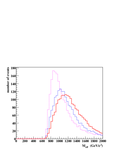
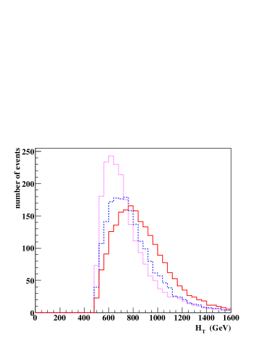
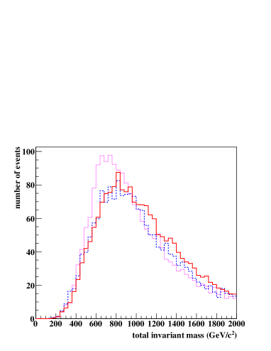
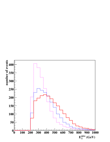
Our approach to kinematic observables in small data sets (low luminosity) is to define inclusive counts based on large bins. The dependence on the details of the detector simulation is strongly reduced by limiting the number of bins and using a bin width much larger than the expected detector resolution.

For $M_{\rm eff}$ we define two bins and one new inclusive count for the kinematic distributions in each box:

• N(Meff1400) the number of events after selection with $M_{\rm eff}>1400$ GeV/$c^{2}$.

For $H_{T}$ we also define two bins and one new inclusive count:

• N(HT900) the number of events after selection with $H_{T}>900$ GeV/$c^{2}$.

Recall that the $E_{T}^{\rm{miss}}$ selection already required $H_{T}>500$ GeV. For the invariant mass $M$ we define three bins and two new inclusive counts:

• N(M1400) the number of events after selection with $M>1400$ GeV/$c^{2}$;

• N(M1800) the number of events after selection with $M>1800$ GeV/$c^{2}$;

For $E_{T}^{\rm{miss}}$ we define four bins and three new inclusive counts:

• N(MET320), the number of events after selection having $E_{T}^{\rm{miss}}$$>320$ GeV.

• N(MET420), the number of events after selection having $E_{T}^{\rm{miss}}$$>420$ GeV.

• N(MET520), the number of events after selection having $E_{T}^{\rm{miss}}$$>520$ GeV.

Note that the $E_{T}^{\rm{miss}}$ selection already required $E_{T}^{\rm{miss}}$$>220$ GeV.

V.3 Kinematic peaks and edges

With large signal samples, kinematic edges involving leptons will be a powerful tool for model discrimination and to eventually extract the mass spectrum of the heavy partners. With small samples, in the range of 100 pb^-1 to 1000 pb^-1 considered in our study, this will only be true in favorable cases. In fact for the 8 models studied here, we find no discrimination at all based on kinematic edges with leptons. This is due mostly to the small number of high $p_{T}$ muons in our signal samples , as well as a lack of especially favorable decay chains.

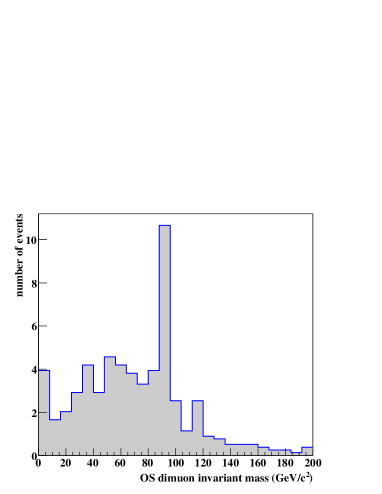
Although we do not observe any dimuon edges, we do see a dimuon peak for model LM8. This is shown in Figure (14), for signal events after our missing energy selection rescaled to 1000 pb^-1 of integrated luminosity. A $Z$ peak is clearly visible, arising from squark decays to quark $+\tilde{\chi}_{2}^{0}$, with the $\tilde{\chi}_{2}^{0}$ decaying 100% to $Z+$ LSP.

Figure 14: The invariant mass distribution for opposite sign dimuon pairs passing the missing energy selection, from MSSM model LM8. The plot is from 100,000 generated events rescaled to 1000 pb^-1.

V.4 Event shapes, hemispheres and cones

Event shapes are a way to extract information about the underlying partonic subprocess and the resulting decay chains. This information is not uncorrelated with kinematics, but it does have the potential to provide qualitatively new characteristics and properties of the event topology. For our signal the partonic subprocess consists of the production of two heavy partner particles, so each event has a natural separation into two halves that we will call “hemispheres”, consisting of all of the decay products of each partner. Associated to each hemisphere of the event should be one WIMP plus some number of reconstructed jets and muons. A perfect hemisphere separation is thus an associative map of each reconstructed object into one of the two constituent decay chains.

We can define two hemisphere axes in $\eta$-$\phi$ as the directions of the original parent particles; these axes are not back-to-back because of the longitudinal (and transverse) boosts from the subprocess center-of-mass frame back to the lab frame. Even if we knew event by event how to boost to the center-of-mass frame, the hemisphere separation would still not be purely geometrical, since in some events a decay product of one parent will end up in the geometrical hemisphere of the other parent.

Having defined a perfect hemisphere separation, we need a practical algorithm to define reconstructed hemispheres. We will follow a study of 6 hemisphere algorithms presented in the CMS Physics TDR Ball:2007zza . These algorithms are geometrical and kinematic, based on the large though imperfect correlation between the $\eta$-$\phi$ vector of the initial parent and the reconstructed objects from this parent’s decay chain. The algorithms consist of two steps: a seeding method that estimates the two hemisphere axes, and an association method that uses these two axes to associate each reconstructed object to one hemisphere.

For the Group 1 model LM5, the CMS study found that jets were correctly associated to parent squarks 87% of the time, and to parent gluinos 70% of the time. The differences in the performance of the 6 algorithms were small; the best-performing hemisphere algorithm combines the following methods:

• Seeding method: The two hemisphere axes are chosen as the $\eta$-$\phi$ directions of the pair of reconstructed objects with the largest invariant mass. The hardest of these objects defines the leading hemisphere.

• Association method: A reconstructed object is assigned to the hemisphere that minimizes the Lund distance Ball:2007zza .

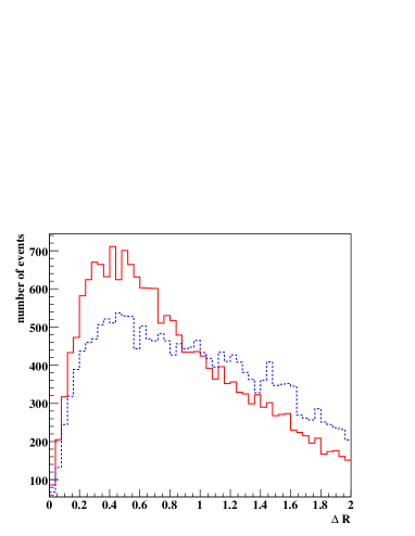
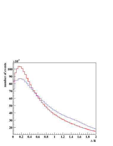
Figure 15 shows how well the seeding method produces hemisphere axes that match the actual axes defined by the two parent particles. The separation is shown in units of $\Delta R$, defined as

$$\Delta R\equiv\sqrt{(\Delta\eta)^{2}+(\Delta\phi)^{2}}\;.$$ (4)

The agreement is not overwhelmingly good, and is substantially worse than that obtained for $t\bar{t}$ events, as shown in Figure 16. We have checked that all 6 hemisphere algorithms produce very similar results. Since the agreement is better for the leading hemisphere, all of our single hemisphere derived observables are based just on the leading hemisphere.

We define three inclusive counts based on comparing the two reconstructed hemispheres:

• N(Hem$j$) the number of events for which the reconstructed object multiplicity (jets + muons) in the two hemispheres differs by at least j, j=1,2,3.

Once the two hemispheres are identified, we can break the degeneracy among the models by looking at the topology in the events. For a given mass of the parent particles, the events will look more jet-like rather than isotropic if the decays are two-body rather than multibody cascades. In the case of jet-like events, the projection of the observed track trajectories on the transverse plane will cluster along the transverse boost of the particles generating the cascade.

In order to quantify this behaviour, we start from the central axes of each hemisphere and draw slices in the transverse plane with increasing opening angles in $\phi$ symmetric around the hemisphere axis. We refer to the slices as cones, reminiscent of the cones used in CLEO analyses cleo to discriminate between jet-like QCD background and isotropic decays of $B$ meson pairs.

We build five cones of opening angle $2\alpha$ ($\alpha$ $=$ $30^{\circ}$, $45^{\circ}$, $60^{\circ}$, $75^{\circ}$ and $90^{\circ}$) in each hemisphere. In terms of these cones we define variables:

• N(nt-c$\alpha$), the number of events having at least n tracks (n=10,20,30,40) in the leading hemisphere cone of opening angle $2\alpha$.

• N(ntdiff-c$\alpha$), the number of events having a difference of at least n tracks (n=10,20,30,40) between the cones of opening angle $2\alpha$ in each hemisphere.

Tracks are counted if they have $p_{T}>1$ GeV/$c$ and $|\eta|<2.4$. Since the cone of opening angle $2\alpha$ includes the one of opening angle $2\beta$ for $\alpha>\beta$, these variables have an inclusive nature.

Figure 15: The distribution of the $\Delta R$ separation between the $\eta$-$\phi$ direction of the parent superpartner and the reconstructed hemisphere axis. This is from 24,667 events of model LM5 passing our selection. The solid red line is for the leading hemisphere, while the dashed blue line is for the second hemisphere.

Figure 16: The distribution of the $\Delta R$ separation between the $\eta$-$\phi$ direction of the parent top quark and the reconstructed hemisphere axis. This is from 3,000,000 Pythia $t\bar{t}$ events with no selection. The solid red line is for the leading hemisphere, while the dashed blue line is for the second hemisphere.

V.5 The stransverse mass $m_{T2}$

A potentially powerful observable for model discrimination and mass extraction is the stransverse mass variable $m_{T2}$ Lester:1999tx -Barr:2003rg . Let us briefly review how this is supposed to work for our missing energy signal. Ignoring events with neutrinos, our signal events have two heavy parent particles of mass $m_{\rm p}$, each of which contributes to the final state a WIMP of mass $m_{\rm dm}$ plus some number of visible particles. Supposing also that we have a perfect hemisphere separation, we can reconstruct each set of visible particles into a 4-vector $p^{X}_{\mu}$. If we also knew the mass and the $p_{T}$ of each WIMP, we could reconstruct a transverse mass for each hemisphere from the formula

$$m_{T}^{2}=m_{X}^{2}+m_{\rm dm}^{2}+2(E^{X}_{T}\,E^{\rm dm}_{T}-\mathbf{p}^{X}_{T}\cdot\mathbf{p}^{\rm dm}_{T})\;.$$ (5)

This transverse mass is always less than or equal to the mass $m_{\rm p}$ of the parent particle. Thus the largest of the two transverse masses per event is also a lower bound on $m_{\rm p}$.

Of course we do not know the $p_{T}$ of each WIMP, only the combined $E_{T}^{\rm{miss}}$. Let $p_{T}^{(1)}$ and $p_{T}^{(2)}$ denote a possible decomposition of the total $p_{T}^{\rm miss}$ into two azimuthal vectors, one for each WIMP. Note that this decomposition ignores initial state radiation, the underlying event and detector effects. Then we can define the stransverse mass of an event as

$$m_{T2}^{2}(m_{\rm dm})\equiv$$ (6)

$${\rm min}\kern-26.0pt\lower 15.0pt\hbox{$\scriptstyle p_{T}^{(1)}+p_{T}^{(2)}=p_{T}^{\rm miss}$}\;\left[{\rm max}\left[m_{T2}^{2}(m_{\rm dm};p_{T}^{(1)}),m_{T2}^{2}(m_{\rm dm};p_{T}^{(2)})\right]\right].$$

Since (with the caveats above) one of these partitions is in fact the correct one, this quantity is also a lower bound on the parent mass $m_{\rm p}$.

For a large enough data sample, with the caveats above and ignoring finite decay widths, the upper endpoint of the stransverse mass distribution saturates at the parent mass $m_{\rm p}$, provided we somehow manage to input the correct value of the WIMP mass $m_{\rm dm}$. In the approximation that the invariant mass $m_{X}$ of the visible decay products is small, the lower endpoint of the stransverse mass distribution is at $m_{\rm dm}$.

These impressive results seem to require that we know a priori the correct input value for $m_{\rm dm}$. However it has been shown Cho:2007qv -Barr:2007hy that in principle there is a kink in the plot of the upper endpoint value of $m_{T2}$ as a function of the assumed $m_{\rm dm}$, precisely when the input value of $m_{\rm dm}$ equals its true value. Thus it may be possible to extract both $m_{\rm p}$ and $m_{\rm dm}$ simultaneously.

Summarizing the remaining caveats, the stransverse mass method requires a large data sample, and is polluted by effects from incorrect hemisphere separation, ISR, the underlying event, finite decay widths and detector effects. We can compare this to the precision extraction of the $W$ mass at CDF CDF:2007ypa ; Aaltonen:2007ps , using the transverse mass distribution of the charged lepton and neutrino from the $W$ decay. Here the WIMP mass is essentially zero, the data samples are huge, and hemisphere separation is not applicable since there is only one WIMP. In the CDF analysis the ISR uncertainty was traded for an FSR uncertainty, by interpreting the vector sum of all the calorimetric $E_{T}$ not associated with the charged lepton as coming from ISR plus the underlying event; this then pollutes the reconstructed neutrino $p_{T}$ with final state radiation from the lepton. The measured transverse mass distribution has a considerable tail extending above the putative endpoint at $m_{W}$, but a precision mass (and width) extraction is still possible by modeling the distribution.

Figure 17: Comparison of the stransverse mass $m_{T2}$ distributions for model CS6, varying the cut on the maximum hemisphere invariant mass. The solid red line shows the $m_{T2}$ distribution when no cut is applied. The dashed blue line shows the $m_{T2}$ distribution rejecting events when the total reconstructed invariant mass of either hemisphere exceeds 300 GeV. The dotted magenta line shows the $m_{T2}$ distribution when this cut is lowered to 200 GeV. In each case 100,000 events were generated then rescaled to 1000 pb^-1. The dotted horizontal lines are to guide the eye for where the distribution cuts off for 100 pb^-1 and 1000 pb^-1.

Figure 18: Comparison of the stransverse mass $m_{T2}$ distributions for look-alike models LM2p (solid red line) and CS6 (dashed blue line). For each model 100,000 events were generated then rescaled to 1000 pb^-1. The dotted horizontal lines are to guide the eye for where the distribution cuts off for 100 pb^-1 and 1000 pb^-1.

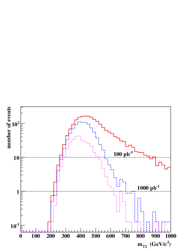
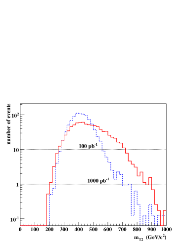
In Nojiri:2008hy it was shown that an imperfect hemisphere separation greatly degrades the $m_{T2}$ distribution for simulated LHC SUSY events. Two approaches to solve this problem have been suggested. The first, used in Nojiri:2008hy , is to reject events when the total invariant mass of the reconstructed objects in either hemisphere exceeds some value. This strategy is based on the fact that for a correct hemisphere separation with $m_{T2}$ near the endpoint the hemisphere invariant mass is small, while incorrect hemisphere assignments naturally lead to large hemisphere invariant masses. The second approach, used in Lester:2007fq , is to replace $m_{T2}$ with a new variable $m_{TGen}$. The new variable minimizes not only over all partitions of the $p_{T}^{\rm miss}$ into $p_{T}^{(1)}$ and $p_{T}^{(2)}$, but also over all possible hemisphere assignments. Since one of the hemisphere separations is in fact the correct one, $m_{TGen}$ has the same endpoint as $m_{T2}$ would have with a perfect hemisphere separation.

Figure 17 shows the degradation of the $m_{T2}$ distribution for our model CS6. The $m_{T2}$ endpoint should be at 589 GeV, the value of the gluino mass in CS6. However the solid red line shows that a large fraction of events are above this endpoint, due to the imperfect hemisphere separation. Applying the strategy of Nojiri:2008hy , the dotted magenta line shows that we regain the correct endpoint by making a hard cut of 200 GeV on the maximum reconstructed hemisphere invariant mass. However with such a high requirement we take a big hit in statistics. The dashed blue line shows that we still do pretty well with a 300 GeV requirement, while gaining a lot in statistics. For this study we have used the 300 GeV requirement in all of our $m_{T2}$ analysis. The value is unoptimized but also unbiased, since it was determined by asking for approximately the most stringent cut that retains reasonable statistics for the $m_{T2}$ distributions of the entire set of models considered.

Figure 18 shows a comparison of the $m_{T2}$ distributions for two of our Group 1 look-alike models, LM2p and CS6. For LM2p, the parents are gluinos of mass 856 GeV and squarks of mass approximately 800 GeV; for model CS6, by contrast, the parents are gluinos of mass 589 GeV. In each case we have input the correct LSP mass, 142 GeV for LM2p and 171 GeV for CS6.

Each plot is rescaled to 1000 pb^-1. With this many events notice that we are just starting to saturate the appropriate endpoints at $m_{T2}=m_{\rm p}$, and notice the onset of tails above the endpoints. The dotted lines in the figure guide the eye to where the distributions cut off for data samples of 100 pb^-1 and 1000 pb^-1. Obviously for 100 pb^-1 we are not close to populating the endpoints.

However even for 100 pb^-1 there are significant differences between the $m_{T2}$ distributions of the two models. These differences only become larger if we use the same input mass for the LSP. Thus $m_{T2}$ is at least as interesting for look-alike discrimination as the more traditional kinematic variables discussed above. Furthermore, even if we are not close to populating the endpoint, it might be possible to extract a direct estimate of $m_{\rm p}$ by fitting or extrapolating the distributions.

For our study we define five bins and four new inclusive counts from $m_{T2}$:

• N(mT2-300) the number of events after selection with $m_{T2}>300$ GeV/$c^{2}$,

• N(mT2-400) the number of events after selection with $m_{T2}>400$ GeV/$c^{2}$,

• N(mT2-500) the number of events after selection with $m_{T2}>500$ GeV/$c^{2}$.

• N(mT2-600) the number of events after selection with $m_{T2}>600$ GeV/$c^{2}$.

When comparing a model M1, playing the role of the data, with a model M2, playing the role of the model to test, we will use the mass of the WIMP in model M2 as the input mass in calculating $m_{T2}$ for both models.

V.6 Flavor enrichment

In order to have some model discrimination based on the $\tau$ or $b$ content, we need simple algorithms to create subsamples enriched with $b$ quarks and $\tau$’s. We refer to these algorithms as “tagging”, despite the fact that the tagging efficiencies and the purity of the subsamples are rather poor.

Without attempting any detailed optimizations, we have designed two very simple tagging algorithms. We expect these algorithms to be robust, since they only require a knowledge of uncorrected high $E_{T}$ jets, high $p_{T}$ muons, and basic counting of high $p_{T}$ tracks inside jets.

$\mathbf{\tau}$ enrichment: For each jet we define a 0.375 cone centered around the jet axis. Inside this cone we count all reconstructed charged tracks with $p_{T}>2$ GeV/$c$. If only one such track is found, and if this track has $p_{T}>15$ GeV/$c$, we tag the jet as a $\tau$ jet.

The $\tau$ algorithm is based on single-prong hadronic $\tau$ decays, which as their name implies produce a single charged track. In addition, leptonic decays of a $\tau$ to an electron and two neutrinos can be tagged, since some fraction of electrons reconstruct as jets. Soft tracks with $p_{T}\leq 2$ GeV/$c$ are not counted, a fact that makes the algorithm much more robust. The $p_{T}>15$ GeV/$c$ requirement on the single track reduces the background from non-$\tau$ jets. Increasing the cone size decreases the efficiency to tag genuine $\tau$’s, because stray tracks are more likely to be inside the cone; decreasing the cone size increases the fake rate. A genuine optimization of this algorithm can only be done with the real data.

Table 19 shows the results of applying our $\tau$ tagging algorithm to simulations of the Group 1 models LM2p, LM5, LM8, CS4d and CS6. The efficiency, defined as the number of $\tau$ tags divided by the number of generator-level $\tau$’s that end up reconstructed as jets, varies between 12% and 21%. The efficiency is lowest for models LM8 and CS4d, models where $\tau$’s come entirely from $W$ and $Z$ decays. The efficiency is highest for model LM2p, which has a large final state multiplicity of $\tau$’s from decays of charginos, second neutralinos and staus.

The purity, defined as the fraction of $\tau$ tagged jets that actually correspond to generator-level $\tau$’s, is quite low for models LM8 and CS4d, and is only 8% for model CS6, which contains very few $\tau$’s. We obtain a reasonably high purity of 55% for LM2p, the model with by far the largest $\tau$ multiplicity.

We conclude that it is possible to obtain significantly enriched samples of $\tau$’s from our simple algorithm, but only for models that do have a high multiplicity of energetic $\tau$’s to begin with. From the counts in Table 19, it is clear that this tagging method is not viable with 100 pb^-1 of integrated luminosity.

Table 19: Results of our $\tau$ tagging algorithm applied to the Group 1 models LM2p, LM5, LM8, CS4d and CS6. Counts are rescaled to 1000 pb^-1 from 100,000 events per model. The listing for $\tau$ jets counts generator level $\tau$’s that are reconstructed as jets in events that pass our selection.

	LM2p	LM5	LM8	CS4d	CS6
$\tau$ jets per fb-1	409	144	171	112	34
tags per fb-1	157	110	122	102	59
correct
tags per fb-1	86	25	21	14	5
efficiency	21%	18%	12%	13%	16%
purity	55%	23%	17%	14%	8%

$\mathbf{b}$ enrichment: For each jet we search for a reconstructed muon inside the jet (recall that our muons have $p_{T}>20$ GeV/$c$ and $|\eta|<2.4$). If a muon is found within $\Delta R<0.2$ of the jet axis we tag it as a $b$ jet.

This $b$ algorithm is based on tagging muons from semileptonic $B$ decays inside the $b$ jet. This is inspired by the “soft muon” tagging that was used in the top quark discovery at the Tevatron Abe:1995hr ; Abachi:1995iq . In our case “soft” is a misnomer, since in fact we only count reconstructed muons with $p_{T}>20$ GeV/$c$. This requirement makes the tagging algorithm more robust, but reduces the efficiency.

Table 20 shows the results of applying our $b$ tagging algorithm to simulations of the Group 1 models LM2p, LM5, LM8, CS4d and CS6. The tagging efficiency is defined as the number of $b$ tags divided by the number of generator-level $b$’s that are within $\Delta R<0.3$ of the center of a reconstructed jet. Although all of these models have a high multiplicity of generator-level $b$’s, the tagging efficiency is poor: only about 5% for all models. However the purity of the samples is rather good: above 70% for every model except CS6.

We conclude that it is possible to obtain significantly enriched samples of $b$’s from our simple algorithm, but with low efficiency. From the counts in Table 20, it is clear that this tagging method is not viable with 100 pb^-1 of integrated luminosity, but should become useful as we approach 1000 pb^-1.

In our study, discrimination based on $\tau$’s and $b$’s is obtained from ratios that involve the following two inclusive counts:

• N($\tau$-tag), the number of events after selection having at least one $\tau$ tag.

• N($b$-tag), the number of events after selection having at least one soft muon $b$ tag.

Table 20: Results of our $b$ tagging algorithm applied to the Group 1 models LM2p, LM5, LM8, CS4d and CS6. Counts are rescaled to 1000 pb^-1 from 100,000 events per model. The listing for $b$ jets counts generator level $b$ quarks matched to reconstructed jets that pass our selection.

	LM2p	LM5	LM8	CS4d	CS6
$b$ jets per fb-1	1547	1693	2481	1596	748
tags per fb-1	115	112	148	105	106
correct
tags per fb-1	82	81	112	75	41
efficiency	5%	5%	5%	5%	5%
purity	72%	72%	75%	71%	39%

VI The look-alike analysis

The look-alike analysis proceeds in four steps:

1. We choose one of the models to play the part of the data. We run the inclusive $E_{T}^{\rm{miss}}$+jets analysis on the MET trigger and verify that the predicted yield establishes an excess (at $>5\sigma$) above the SM background with $100$ pb^-1. We call the number of events selected in this way the observed yield $N_{\rm data}$. In what follows, we assume that a subtraction of the residual Standard Model background has already been performed. We assume large signal over background ratios for the models considered so that the statistical error on the background has a small impact on the total error.

2. We identify a set of models giving a predicted yield $N$ compatible with $N_{\rm data}$. The compatibility is established if the difference in the two counts is less than twice the total error, i.e if the pull

$$\frac{|N_{\rm data}-N|}{\sigma(N)}$$ (7)

is smaller that two. In the formula $\sigma(N)$ represents the error associated to the expected number of events $N$. We calculate it as the sum in quadrature of several contributions:

• A Poissonian error which takes into account the statistical fluctuations associated to the event production (statistical component of the experimental error).

• An error associated to the detector effects (systematic component of the experimental error).

• Theoretical error on the predicted number of events $N$ (including a statistical and a systematic component).

We discuss the origin of each contribution below.

3. For each additional observable $N^{i}$ previously listed, we consider the value on the data ($N^{i}_{\rm data}$) and the predicted value $N^{i}_{j}$ for the model $j$. We calculate the pull as in eqn. 7 and we identify the variable with the largest pull as the best discriminating counting variable. We ignore all the variables for which both the model and the data give a yield below a fixed threshold $N_{\rm min}$. We use $N_{\rm min}=10$, i.e. we require a minimum yield that is more than three times its Poisson error $\sqrt{N^{i}}$; for the data this corresponds to excluding at 3$\sigma$ the possibility that the observed yield is generated by a fluctuation of the background.

4. We form ratios of some of the observables used above and we repeat the procedure of step 3. Since part of the uncertainties cancel out in the ratio, these variables allow a better discrimination than the counting variables. In addition, provided that the two variables defining the ratio are above the threshold $N_{\rm min}$, the ratios of two correlated variables (such as $N(4j)/N(3j)$) are less sensitive to the statistical fluctuations. Details on the calculation of the errors on the ratios are given below.

In each of the four trigger boxes we define the following ratios of correlated inclusive counts:

• r($n$j)(3j), with n=4,5

• r(MET320)

• r(MET420)

• r(MET520)

• r(HT900)

• r(Meff1400)

• r(M1400)

• r(M1800)

• r(Hem$j$) with $j$=1,2,3

• r(2$\mu$-nj)(1$\mu$-nj) with n=3,4

• r($\tau$-tag)

• r($b$-tag)

• r(mT2-300) with the theory LSP mass

• r(mT2-400) with the theory LSP mass

• r(mT2-500) with the theory LSP mass

• r(mT2-600) with the theory LSP mass

• r(mT2-400/300) with the theory LSP mass

• r(mT2-500/300) with the theory LSP mass

• r(mT2-600/300) with the theory LSP mass

• r(nt-c$\alpha$) for n=10,20,30,40 and $\alpha=30^{\circ}$,$45^{\circ}$, $60^{\circ}$, $75^{\circ}$, $90^{\circ}$

• r(ntdiff-c$\alpha$) for for n=10,20,30,40 and $\alpha=30^{\circ}$, $45^{\circ}$, $60^{\circ}$, $75^{\circ}$, $90^{\circ}$

For most of these ratios the numerator is the corresponding count defined in Section V and the denominator is the total event count in the trigger box. The exceptions are r($n$j)(3j)$=$N($n$j)/N(3j), r(2$\mu$-nj)(1$\mu$-nj)$=$N(2$\mu$-nj)/N(1$\mu$-nj), and r(mT2-$n$/300)$=$N(mT2-$n$)/N(mT2-300), $n=400,500,600$. We also use the ratios of the counts in the DiJet, TriJet and Muon20 boxes to the count in the MET box:

• r(DiJet)

• r(TriJet)

• r(Muon20)

As mentioned previously, it turns out that the DiJet, TriJet and Muon20 boxes are subsamples of the MET box to an excellent approximation, thus these ratios are also ratios of inclusive counts.

Finally we iterate and perform the transpose comparisons (the model that was considered as data takes the role of the model).

VI.1 Theoretical uncertainty

We take into account several sources of uncertainty. First of all, there is an error associated to the knowledge of the parton probability density functions (pdfs) that are used to generate the event samples. In order to evaluate this error, we produce and analyze all samples with three different sets of pdfs: CTEQ5L cteq , CTEQ6M cteq , and MRST2004nlo MRST or MRST2002nlo MRST for Group 1 and Group 2 respectively. We quote as central value the average of the three values; for the pdf uncertainty we crudely estimate it by taking half the spread of the three values. This uncertainty, as we will show, has important effects on the results.

An additional error is given by the relative QCD scale uncertainty when we compare different look-alike models. This is an overall systematic on the relative cross sections that we take to be $5\%$. It is actually larger than this in our study, at least for the Group 2 models where we use LO cross sections, but we are assuming some improvement by the time of the real discovery.

There is an additional uncertainty for each observable from the missing higher order matrix elements. It is not included in the analysis shown here. It could be included crudely by running Pythia with different values of the ISR scale controlled by MSTP(68), similar to how we evaluate the pdf uncertainties. A better way is to include, for the signals, the higher order matrix elements for the emission of extra hard jets. The ideal approach would be a full NLO generator for the signals.

The sum in quadrature of all these effects gives the systematic error associated to the theoretical prediction. In the case of ratios, the error on the cross section cancels out. In a similar way, the correlated error on the pdfs cancels out by calculating the ratios for the three sets of pdfs and then averaging them.

In the case of mSUGRA models, the result of the simulation also depends on which RGE evolution code we use to go from the parameters at the high scale to the SUSY spectrum at the Terascale. Rather than including an error associated to such differences we take one of the codes (Isajet v7.69 or SuSpect v2.34) as part of the definition of the theory model we are considering.

The theory predictions are also affected by a statistical error, related to the fact that the value of each observable is evaluated on a sample of limited size. Generating the same sample with a different Monte Carlo seed one obtains differences on the predicted values of the observable. The differences, related to statistical fluctuations, are smaller for larger generated data sets. Considering that each number of events $N_{i}^{j}$ for observable $i$ and model $j$ can be written as $N_{i}^{j}=\epsilon_{i}^{j}\times\sigma^{j}$ and that the error on $\sigma^{j}$ is already accounted for in the systematic contribution to the theoretical error, the efficiency $\epsilon_{i}^{j}$ has an associated binomial error:

$$\sigma(\epsilon_{i})=\sqrt{\frac{\epsilon_{i}^{j}\times(1-\epsilon_{i}^{j})}{N_{\rm GEN}}}$$ (8)

where $N_{\rm GEN}$ is the size of the generated sample before any selection requirement. This error can be made negligible by generating data sets with large values of $N_{\rm GEN}$. We include the contribution of the statistical error summing it in quadrature to the systematic error.

When the variables defining the ratio are uncorrelated, the error on the ratio is obtained by propagating the errors on the numerator and denominator, according to the relation

$$\sigma(r)=\sqrt{\left(\frac{\sigma(N_{\rm num})}{N_{\rm den}}\right)^{2}+\left(\frac{N_{\rm num}\sigma(N_{\rm den})}{N_{\rm den}^{2}}\right)^{2}}$$ (9)

where $r=N_{\rm num}/N_{\rm den}$.

This is not the correct formula in our case, since all of the counts on our ratios are correlated. For instance, $N(4j)$ and $N(3j)$ are correlated, since all the events with at least four jets have also three jets. Only a fraction of the events defining $N(3j)$ will satisfy the requirement of an additional jet, i.e. applying the requirement of an additional jet on the $\geq 3$ jets sample corresponds to a binomial process, with the ratio $r(4j)(3j)=N(4j)/N(3j)$ the associated efficiency. The error on $r$ is then given by eqn. 8, replacing $\epsilon_{i}^{j}$ with the $r$ and $N_{\rm GEN}$ with $N(4j)$. The same consideration applies to all the ratios built from correlated variables. In order to use eqn. 8 for the error, we always define the ratios such that they are in the range [0,1].

VI.2 Statistical uncertainty

The production of events of a given kind in a detector is a process ruled by Poisson statistics. The error on a counting variable $N$ is given by $\sqrt{N}$.

In analogy to the statistical error on the theoretical predictions, the statistical error on a ratio of two correlated variables is calculated according to eqn. 8, replacing $\epsilon_{i}^{j}$ with the $r$ and $N_{\rm GEN}$ with the value of the denominator variable for the reference data luminosity. Unlike the case of the theoretical error, this error is associated to the statistics of the data set and not to the size of the generated sample; this error is intrinsic to the experimental scenario we are considering and cannot be decreased by generating larger Monte Carlo samples.

VI.3 Systematic uncertainty

We consider two main sources of systematic error, the knowledge of the collected luminosity and the detector effects on the counting variables. Estimating the two contributions to be of the order of $10\%$, we assign a global systematic error of $15\%$ to the counting variables. When calculating the ratios, we expect this error to be strongly reduced. On the other hand the cancellation is not exact, and it will be less effective at the start-up, because of potentially poorly-understood features related to the reconstruction. Hence we associate a residual systematic error of $5\%$ to the ratios.

Table 21: Summary of the best discriminating ratios for model comparisons in Group 1. The models listed in rows are taken as simulated data, with either 100 or 1000 pb^-1 of integrated luminosity assumed, and uncertainties as described in the text. The models listed in columns are then compared pairwise with the “data”. In each case, the three best distinct discriminating ratios are shown, with the estimated significance. By distinct we mean that we only list the best ratio of each type; thus if r(5j)(4j) is listed, then r(4j)(3j) is not, etc. The asterix on the ratio r($b$-tag) indicates that it is defined in the Muon20 box; all other ratios are defined in the MET box, and r(Muon20) denotes the ratio of the number of events in the Muon20 box to the number in the MET box. The $m_{T2}$ ratios are computed using the LSP mass of the relevant “theory” model, not the “data” model.

	LM2p		LM5		LM8		CS4d		CS6
LM2p
100			r(5j)(3j)	1.6$\sigma\hskip 4.0pt$	r(5j)(3j)	4.4$\sigma\hskip 4.0pt$	r(MET520)	4.1$\sigma\hskip 4.0pt$	r(mT2-600/300)	11.4$\sigma\hskip 4.0pt$
			r(mT2-300)	1.4$\sigma\hskip 4.0pt$	r(MET520)	3.7$\sigma\hskip 4.0pt$	r(HT900)	3.6$\sigma\hskip 4.0pt$	r(MET520)	10.6$\sigma\hskip 4.0pt$
			r($\tau$-tag)	1.2$\sigma\hskip 4.0pt$	r(10t-c45)	2.9$\sigma\hskip 4.0pt$	r(Meff1400)	3.0$\sigma\hskip 4.0pt$	r(HT900)	6.8$\sigma\hskip 4.0pt$
1000			r($\tau$-tag)	3.1$\sigma\hskip 4.0pt$	r(MET520)	8.2$\sigma\hskip 4.0pt$	r(MET520)	9.4$\sigma\hskip 4.0pt$	r(mT2-600/300)	33.0$\sigma\hskip 4.0pt$
			r(5j)(3j)	2.8$\sigma\hskip 4.0pt$	r(mT2-500)	6.7$\sigma\hskip 4.0pt$	r(HT900)	6.4$\sigma\hskip 4.0pt$	r(MET520)	26.6$\sigma\hskip 4.0pt$
			r(mT2-400)	2.6$\sigma\hskip 4.0pt$	r(5j)(3j)	6.5$\sigma\hskip 4.0pt$	r(mT2-600)	6.0$\sigma\hskip 4.0pt$	r(HT900)	14.6$\sigma\hskip 4.0pt$
LM5
100	r(5j(3j)	1.8$\sigma\hskip 4.0pt$			r(5j)(3j)	2.9$\sigma\hskip 4.0pt$	r(HT900)	3.6$\sigma\hskip 4.0pt$	r(mT2-600/300)	11.6$\sigma\hskip 4.0pt$
	r(mT2-300)	1.5$\sigma\hskip 4.0pt$			r(MET520)	2.7$\sigma\hskip 4.0pt$	r(Meff1400)	3.2$\sigma\hskip 4.0pt$	r(MET520)	9.2$\sigma\hskip 4.0pt$
	r(10t-c30)	1.4$\sigma\hskip 4.0pt$			r(Muon20)	2.5$\sigma\hskip 4.0pt$	r(MET520)	3.1$\sigma\hskip 4.0pt$	r(HT900)	6.8$\sigma\hskip 4.0pt$
1000	r(5j)(4j)	3.4$\sigma\hskip 4.0pt$			r(MET520)	6.0$\sigma\hskip 4.0pt$	r(MET520)	7.1$\sigma\hskip 4.0pt$	r(mT2-600/300)	33.7$\sigma\hskip 4.0pt$
	r($\tau$-tag)	2.7$\sigma\hskip 4.0pt$			r(Muon20)	4.9$\sigma\hskip 4.0pt$	r(HT900)	6.4$\sigma\hskip 4.0pt$	r(MET520)	22.9$\sigma\hskip 4.0pt$
	r(mT2-400)	2.6$\sigma\hskip 4.0pt$			r(5j)(3j)	4.3$\sigma\hskip 4.0pt$	r(mT2-600/400)	6.1$\sigma\hskip 4.0pt$	r(HT900)	14.6$\sigma\hskip 4.0pt$
LM8
100	r(5j)(3j)	5.5$\sigma\hskip 4.0pt$	r(5j)(3j)	3.3$\sigma\hskip 4.0pt$			r(5j)(3j)	3.1$\sigma\hskip 4.0pt$	r(Muon20)	10.1$\sigma\hskip 4.0pt$
	r(10t-c30)	3.7$\sigma\hskip 4.0pt$	r(Muon20)	3.1$\sigma\hskip 4.0pt$			r(mT2-400)	2.2$\sigma\hskip 4.0pt$	r(mT2500/300)	5.2$\sigma\hskip 4.0pt$
	r(Muon20)	3.6$\sigma\hskip 4.0pt$	r(MET520)	2.4$\sigma\hskip 4.0pt$			r(20t-c45)	2.1$\sigma\hskip 4.0pt$	r(Hem3)	4.1$\sigma\hskip 4.0pt$
1000	r(5j)(3j)	10.1$\sigma\hskip 4.0pt$	r(Muon20)	7.2$\sigma\hskip 4.0pt$			r(5j)(3j)	5.4$\sigma\hskip 4.0pt$	r(Muon20)	25.8$\sigma\hskip 4.0pt$
	r(Muon20)	8.0$\sigma\hskip 4.0pt$	r(Hem3)	5.7$\sigma\hskip 4.0pt$			r(Hem3)	5.3$\sigma\hskip 4.0pt$	r(mT2-600/300)	20.1$\sigma\hskip 4.0pt$
	r(Hem3)	7.3$\sigma\hskip 4.0pt$	r(5j)(3j)	5.6$\sigma\hskip 4.0pt$			r(Muon20)	4.1$\sigma\hskip 4.0pt$	r(Hem3)	14.2$\sigma\hskip 4.0pt$
CS4d
100	r(MET520)	3.5$\sigma\hskip 4.0pt$	r(HT900)	3.0$\sigma\hskip 4.0pt$	r(5j)(3j)	2.8$\sigma\hskip 4.0pt$			r(Muon20)	6.8$\sigma\hskip 4.0pt$
	r(HT900)	3.2$\sigma\hskip 4.0pt$	r(MET520)	2.7$\sigma\hskip 4.0pt$	r(mT2-300)	2.1$\sigma\hskip 4.0pt$			r(MET420)	5.5$\sigma\hskip 4.0pt$
	r(Meff1400)	2.6$\sigma\hskip 4.0pt$	r(Meff1400)	2.6$\sigma\hskip 4.0pt$	r(10t-c30)	1.9$\sigma\hskip 4.0pt$			r(mT2-500/300)	5.2$\sigma\hskip 4.0pt$
1000	r(MET520)	6.5$\sigma\hskip 4.0pt$	r(MET520)	5.1$\sigma\hskip 4.0pt$	r(5j)(3j)	4.2$\sigma\hskip 4.0pt$			r(Muon20)	17.3$\sigma\hskip 4.0pt$
	r(mT2-600)	5.3$\sigma\hskip 4.0pt$	r(mT2-600/400)	4.8$\sigma\hskip 4.0pt$	r(10tdiff-c30)	3.6$\sigma\hskip 4.0pt$			r(mT2-500)	12.8$\sigma\hskip 4.0pt$
	r(HT900)	5.2$\sigma\hskip 4.0pt$	r(HT900)	4.5$\sigma\hskip 4.0pt$	r(Hem3)	3.6$\sigma\hskip 4.0pt$			r(MET520)	11.5$\sigma\hskip 4.0pt$
CS6
100	r(MET420)	7.0$\sigma\hskip 4.0pt$	r(MET420)	6.0$\sigma\hskip 4.0pt$	r($b$-tag)∗	6.5$\sigma\hskip 4.0pt$	r(MET420)	4.3$\sigma\hskip 4.0pt$
	r(mT2-500/300)	5.1$\sigma\hskip 4.0pt$	r(mT2-500/300)	4.6$\sigma\hskip 4.0pt$	r(Muon20)	5.2$\sigma\hskip 4.0pt$	r(Muon20)	4.0$\sigma\hskip 4.0pt$
	r(HT900)	4.8$\sigma\hskip 4.0pt$	r(HT900)	4.5$\sigma\hskip 4.0pt$	r(MET420)	4.0$\sigma\hskip 4.0pt$	r(mT2-500/300)	2.9$\sigma\hskip 4.0pt$
1000	r(MET520)	11.5$\sigma\hskip 4.0pt$	r($b$-tag)∗	11.0$\sigma\hskip 4.0pt$	r($b$-tag)∗	15.6$\sigma\hskip 4.0pt$	r($b$-tag)∗	14.9$\sigma\hskip 4.0pt$
	r($b$-tag)∗	11.2$\sigma\hskip 4.0pt$	r(MET520)	10.3$\sigma\hskip 4.0pt$	r(Muon20)	10.2$\sigma\hskip 4.0pt$	r(Muon20)	8.4$\sigma\hskip 4.0pt$
	r(mT2-500)	10.2$\sigma\hskip 4.0pt$	r(mT2-500)	9.2$\sigma\hskip 4.0pt$	r(MET520)	7.6$\sigma\hskip 4.0pt$	r(MET420)	7.6$\sigma\hskip 4.0pt$

VII Summary of Group 1 results

Table 21 summarizes the results from the five MSSM models of Group 1. There are 20 pairwise model comparisons. One model is taken as the simulated data, with the observed yield scaled to either the 100 pb^-1 discovery data set or a 1000 pb^-1 follow-up. The actual number of events generated in each case was 100,000, thus the “data” has smaller fluctuations than would be present in the real experiment; we are interested in identifying the best discriminators and their approximate significance, not simulating the real experiment. Note, however, that in our analysis we include the correct statistical uncertainty arising from the assumed 100 pb^-1 or 1000 pb^-1 of integrated luminosity in the “data” sample, as described in Section VI.B. When the rescaled counts are below a minimum value, the corresponding ratio is not used in our analysis, as described in step 3 of analysis procedure outlined in Section VI.

Given a “data” model, we can compare it to four theory models. We want to understand to what extent we can reject each theory model, based on discrepancies in our discriminating ratios. With the real LHC data, the test needs to be performed as follows: given Model A and Model B, we will ask if Model A is a better description of the data than Model B; this is a properly posed hypothesis test. Every time we reject a theory model as an explanation of the “data”, we learn something about the true properties of the model underlying the “data”. When several discriminating ratios have high significance, we may learn more than one qualitative feature of the underlying model from a single pairwise comparison; this is not always the case however, since many ratios probe very similar features of the models and are thus highly correlated.

In general the discriminating power of the robust ratios is quite impressive. For 8 of the pairwise comparisons at least one ratio discriminates at better than 5$\sigma$ with only 100 pb^-1 of simulated data. In only three cases (discussed in more detail below) do we fail to discriminate by at least 5$\sigma$ with 1000 pb^-1. In 14 out of 20 cases 1000 pb^-1 gives $>5\sigma$ discrimination with 3 or more different ratios, giving multiple clues about the underlying data model.

Figure 19: Comparison of the stransverse mass $m_{T2}$ distributions for look-alike models LM5 (solid red line) and CS4d (dashed blue line). For each model 100,000 events were generated then rescaled to 1000 pb^-1.

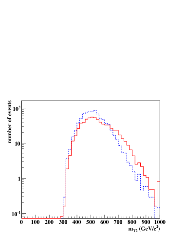
VII.1 LM5 vs CS4d

We begin with one of the simplest pairwise comparisons: LM5 is treated as the data and compared to theory model CS4d. Averaging over the three pdfs used in our study, we find that LM5 would produce 1951 signal events in the 100 pb^-1 discovery sample. This is only 7% more than the 1817 events predicted by theory model CS4d, so the data model and theory model are indeed look-alikes. If we peek at the features of the two models we see that they have a number of phenomenological similarities. Both models have about the same proportion of squark-gluino and squark-squark production. In CS4d gluinos decay to stop-top, followed by the three-body stop decay $\tilde{t}_{1}\rightarrow bW^{+}\tilde{\chi}_{1}^{0}$; this resembles LM5 gluinos decaying to left-squark-quark, followed by left-squark cascade to chargino-quark, with the chargino decaying to $W\tilde{\chi}_{1}^{0}$. Both models have a large fraction of events with $W$’s.

At the moment of discovery CS4d is excluded as an explanation of the LM5 “data” by more than 3$\sigma$ in three kinematic ratios: r(HT900), r(Meff1400) and r(MET520). These ratios discriminate based on the proportion of highly energetic events; their values are about 50% larger for LM5 than for CS4d. This indicates that the LM5 signal arises from production of heavier parent particles. From the superpartner spectra in Figure 5 we see that indeed the gluino mass is about 100 GeV heavier in LM5 than in CS4d, and the lightest squarks are also somewhat heavier. Note that LM5 has a harder $E_{T}^{\rm{miss}}$ distribution even though its LSP mass is $\sim 100$ GeV lighter than that of CS4d.

Since the $m_{T2}$ endpoint is a direct measure of the (largest) parent particle mass, we would expect the $m_{T2}$ ratios to be good discriminators. However as can be seen in Figure 19 with 100 pb^-1 we are hampered by poor statistics near the endpoint. The best $m_{T2}$ ratio is r(mT2-600/300) in the MET box, computed with the LSP mass of CS4d; it is defined as the number of events in the MET box with $m_{T2}>600$ GeV divided by the number of events with $m_{T2}>300$ GeV. This ratio has 2.8$\sigma$ significance with 100 pb^-1.

Making the same comparison at 1000 pb^-1, the significance of r(MET520), r(HT900) and r(Meff1400) as discriminators improves to 7.1, 6.4 and 5.9$\sigma$ respectively. More importantly, two of the $m_{T2}$ ratios, r(mT2-600/300) and r(mT2-600/400), now discriminate at better than 6$\sigma$. We have not attempted to perform a direct extraction of the endpoint, but it is clear that the $m_{T2}$ ratios can compete with the kinematic ratios as discriminators while simultaneously providing more direct information about the underlying $2\rightarrow 2$ parent subprocess.

Although we can reject CS4d conclusively, some qualitative differences between LM5 and CS4d are not resolved. Model CS4d produces more tops, while LM5 produces a lot of Higgs; however Table 20 shows that the number of $b$ jets, $b$ tags and tagged $b$ jets are all about the same. Lacking an explicit reconstruction of tops or Higgs, we do not discriminate these models based on these features.

VII.2 LM2p vs LM5

This is the most difficult pair of look-alikes in our study. From Figure 5 we see that the superpartner spectra are almost identical; the only significant difference is that LM2p has a much lighter stau. As a result, LM2p events are much more likely to contain $\tau$’s, while LM5 events are much more likely to contain $W$’s (mostly from chargino decays).

As Table 21 shows, at the moment of discovery LM5 cannot be ruled out as the explanation of LM2p “data”. Without $\tau$ tagging, we would not have 3$\sigma$ discrimination even with 1000 pb^-1; the best we could do is the jet multiplicity ratio r(5j)(3j) with 2.8$\sigma$: LM5 produces more high multiplicity jet events after selection, because we can get two jets from a $W$ decay in LM5 compared to only one hadronic $\tau$ from a stau decay in LM2p.

Figure 20: Comparison of the stransverse mass $m_{T2}$ distributions for look-alike models LM2p (solid red line) and LM5 (dashed blue line). For each model 100,000 events were generated then rescaled to 1000 pb^-1.

Figure 21: Comparison of the stransverse mass $m_{T2}$ distributions for model LM2p with a fixed number of reconstructed objects (jets or muons): 3 objects (solid red line), 4 objects (dashed blue line) and 5 objects (dotted magenta line). For each case 100,000 events were generated then rescaled to 1000 pb^-1.

Figure 22: Comparison of the stransverse mass $m_{T2}$ distributions for two subsamples of model LM2p: events with neutrinos (solid red line) and events without neutrinos (dashed blue line). A total of 100,000 events were generated, rescaled to 1000 pb^-1, then sorted into the two subsamples.

Table 22: Summary of the best discriminating ratios for model comparisons in Group 2. The models listed in rows are taken as simulated data, with either 100 or 1000 pb^-1 of integrated luminosity assumed, and uncertainties as described in the text. The models listed in columns are then compared pairwise with the “data”. In each case, the three(five) best distinct discriminating ratios for 100(1000) pb^-1 are shown, with the estimated significance. By distinct we mean that we only list the best ratio of each type; thus if r(5j)(4j) is listed, then r(4j)(3j) is not, etc. Square brackets denote ratios defined in the DiJet, TriJet or Muon20 boxes; all other ratios are defined in the MET box, and r(DiJet), r(TriJet) denotes the ratio of the number of events in the DiJet/TriJet boxes to the number in the MET box. The $m_{T2}$ ratios are computed using the LSP mass of the relevant “theory” model, not the “data” model.

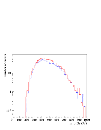
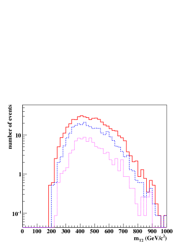
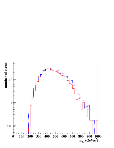
	LH2		NM4		CS7
LH2
100			r(mT2-500)	4.9$\sigma\hskip 4.0pt$	r(mT2-500)	6.7$\sigma\hskip 4.0pt$
			r(Meff1400)	3.0$\sigma\hskip 4.0pt$	r(MET420)	6.5$\sigma\hskip 4.0pt$
			r(M1400)	2.7$\sigma\hskip 4.0pt$	r(4j)(3j)	4.0$\sigma\hskip 4.0pt$
1000			r(mT2-500)	14.1$\sigma\hskip 4.0pt$	r(mT2-500)	18.9$\sigma\hskip 4.0pt$
			r(mT2-300) [TriJet]	11.0$\sigma\hskip 4.0pt$	r(MET420)	16.7$\sigma\hskip 4.0pt$
			r(mT2-400) [DiJjet]	7.9$\sigma\hskip 4.0pt$	r(mT2-500) [TriJet]	8.8$\sigma\hskip 4.0pt$
			r(Meff1400)	7.2$\sigma\hskip 4.0pt$	r(4j)(3j) [DiJet]	7.3$\sigma\hskip 4.0pt$
			r(M1400)	6.6$\sigma\hskip 4.0pt$	r(mT2-300) [DiJet]	6.7$\sigma\hskip 4.0pt$
NM4
100	r(Meff1400)	4.2$\sigma\hskip 4.0pt$			r(Meff1400)	4.3$\sigma\hskip 4.0pt$
	r(M1400)	4.0$\sigma\hskip 4.0pt$			r(DiJet)	4.1$\sigma\hskip 4.0pt$
	r(mT2-400)	3.8$\sigma\hskip 4.0pt$			r(MET420)	4.0$\sigma\hskip 4.0pt$
1000	r(Meff1400)	10.8$\sigma\hskip 4.0pt$			r(Meff1400)	11.2$\sigma\hskip 4.0pt$
	r(TriJet)	10.4$\sigma\hskip 4.0pt$			r(MET520)	10.6$\sigma\hskip 4.0pt$
	r(M1400)	9.8$\sigma\hskip 4.0pt$			r(DiJet)	10.6$\sigma\hskip 4.0pt$
	r(DiJet	8.2$\sigma\hskip 4.0pt$			r(HT900)	9.0$\sigma\hskip 4.0pt$
	r(HT900)	8.0$\sigma\hskip 4.0pt$			r(4j)(3j)	6.1$\sigma\hskip 4.0pt$
CS7
100	r(MET420)	4.9$\sigma\hskip 4.0pt$	r(4j)(3j)	4.4$\sigma\hskip 4.0pt$
	r(4j)(3j)	4.6$\sigma\hskip 4.0pt$	r(MET420)	3.3$\sigma\hskip 4.0pt$
	r(mT2-400)	4.1$\sigma\hskip 4.0pt$	r(Hem1)	3.2$\sigma\hskip 4.0pt$
1000	r(5j)(3j) [DiJet]	16.8$\sigma\hskip 4.0pt$	r(4j)(3j)	9.4$\sigma\hskip 4.0pt$
	r(TriJet)	10.4$\sigma\hskip 4.0pt$	r(5j)(3j) [DiJet]	7.4$\sigma\hskip 4.0pt$
	r(MET420)	9.6$\sigma\hskip 4.0pt$	r(Meff1400)	7.4$\sigma\hskip 4.0pt$
	r(4j)(3j)	9.5$\sigma\hskip 4.0pt$	r(DiJet)	6.9$\sigma\hskip 4.0pt$
	r(mT2-500)	8.3$\sigma\hskip 4.0pt$	r(HT900)	6.2$\sigma\hskip 4.0pt$

With our crude $\tau$ tagging algorithm we manage to discriminate LM2p and LM5 at 3.1$\sigma$ with 1000 pb^-1. As seen in Table 19, the LM2p sample has almost three times as many hadronic $\tau$’s that reconstruct as jets than does the LM5 sample. This results in four times as many jets being correctly tagged as hadronic $\tau$’s, and almost 50% more total $\tau$ tags for LM2p versus LM5.

The only other ratios that give even 2$\sigma$ discrimination are based on the stransverse mass $m_{T2}$. The ratio r(mT2-400) counts the number of events with $m_{T2}>400$ GeV divided by the total number of events after selection; here $m_{T2}$ is computed using the LSP mass of the theory model LM5. Figure 20 compares the $m_{T2}$ distributions of LM2p and LM5. The shapes of the distributions are very similar; the only obvious difference is that there are fewer events in the LM5 bins.

It is not surprising that the shapes are similar, since LM2p and LM5 are very similar models with nearly identical gluino and squark masses. Thus ratios like r(mT2-600/400) should not be good discriminators, and indeed they are not. The ratio r(mT2-400), which is a good discriminator, is obviously just picking up the fact that there are fewer events in the LM5 bins than in the LM2p bins.

Figure 21 compares the $m_{T2}$ distributions of LM2p subsamples with fixed multiplicity of jets$+$muons. We see that events with higher multiplicity are significantly more likely to fail the 300 GeV hemisphere invariant mass upper bound that we imposed to make up for the effect on $m_{T2}$ of imperfect hemisphere separation. This makes sense since events with higher multiplicity are more likely to have mistakes in the hemisphere assignments.

Thus the discriminating power of r(mT2-400) in this case is correlated with r(5j)(3j), not with kinematic ratios like r(HT900) and r(Meff1400).

It is important to note that the $m_{T2}$ ratios have some ability to discriminate based on neutrinos in the final state: Figure 22 shows a comparison of the $m_{T2}$ distributions for LM2p events containing neutrinos versus those without neutrinos. The events with neutrinos have a softer $m_{T2}$ distribution, i.e. the subsample with neutrinos is less efficient at populating the $m_{T2}$ upper endpoint. Models LM2p and LM5 differ greatly in the proportion of events after selection that have neutrinos: about 50% for LM2p but only about 10% for LM5. The neutrino content effect on the $m_{T2}$ distributions actually reduces the discrimination of LM2p versus LM5, because the neutrino effect works in the opposite direction from the dominant effect of jet multiplicity.

This example shows that the interpretation of the $m_{T2}$ ratios requires a comparison with other discriminators. If the $m_{T2}$ ratios r(mT2-xxx/yyy) have a high significance positively correlated with e.g. r(HT900) and r(Meff1400), then the $m_{T2}$ ratios are predominantly indicating kinematics. If the $m_{T2}$ ratios r(mt2-xxx) have a high significance but r(mT2-xxx/yyy) do not (as occurred here), we expect they will be positively correlated with the jet ratios, indicating a difference in the multiplicity of reconstructed objects. If the $m_{T2}$ ratios r(mT2-xxx/yyy) have a high significance uncorrelated or negatively correlated with either kinematics or jet multiplicity, this could signal the presence of three unseen particles (e.g. two LSPs and a neutrino) in the final state of a large fraction of events.

VII.3 CS4d vs LM8

This is the second most difficult pair of look-alikes in our study. From Figure 5 we see that the gluino and squark superpartner spectra are roughly similar. The gluino masses agree to within 10 GeV; in LM8 the left and right squarks are nearly degenerate and slightly heavier than the gluino, while in CS4d the right squarks are slightly lighter than the gluino and the left-squarks are about 180 GeV heavier.

Both models have about the same fractions of squark pair, squark-gluino and gluino pair production after selection. In both models the gluino decays predominately to top-stop. Both models produce many tops, $b$’s and $W$’s. LM8 also produces a lot of $Z$’s from $\tilde{\chi}_{2}^{0}$ decays.

The main difference between these models is that CS4d has a much lighter stop and a much heavier LSP. With $m_{\tilde{t}_{1}}$$=$$352$ GeV and $m_{\tilde{\chi}^{0}_{1}}$$=$$251$ GeV a two-body light stop decay cannot occur, and this stop can just barely manage the three-body decay $\tilde{t}_{1}\rightarrow bW^{+}\tilde{\chi}_{1}^{0}$.

Consider the case that we perform our look-alike analysis taking CS4d as the “data” model and LM8 as the theory model. At the moment of discovery, LM8 will explain not only the overall size of the signal but also its kinematics: with 100 pb^-1 we find no kinematic observable that discriminates better than r(Meff1400) with 1.7$\sigma$, and even with 1000 pb^-1 no kinematic observables discriminate at even the 3$\sigma$ level. Given that LM8 is an mSUGRA benchmark used at the LHC experiments it may be tempting to falsely conclude that LM8 is the probable explanation of the discovery! Since LM8 has 230 GeV charginos, even a preliminary result in this direction could be used, for example, as a justification to start building a 500 GeV linear collider. Since the actual chargino mass of the underlying compressed SUSY model is 352 GeV, this would lead to embarrassment.

Fortunately our look-alike analysis gives additional discriminating handles:

• The ratio r(Muon20) has a 3.4$\sigma$ significance with 1000 pb^-1, reflecting a larger fraction of reconstructed muons in LM8 events over CS4d.

• With 1000 pb^-1 there are enough dimuons to reconstruct the $Z$ peak as shown in Figure 14 for LM8, while no peak appears for CS4d.

• The ratio r(5j)(3j) in the MET box differs by 2.8$\sigma$ at 100 pb^-1, increasing to 4.2$\sigma$ with 1000 pb^-1, reflecting a larger jet multiplicity in LM8 events versus CS4d.

• With 1000 pb^-1 we also see discrepancies in the event shape variables. One of these, r(Hem3), is the fraction of events where the object counts in the two hemispheres differ by at least 3; the other, r(10tdiff-c300), is the fraction of events where the track count in a 30^∘ cone around each hemisphere axis differs by at least 10. With 1000 pb^-1 both these ratios have a significance of 3.6$\sigma$, reflecting more symmetrical object counts in CS4d events than for LM8.

From Table 20 we would have hoped for a significant difference in r($b$-tag) between LM8 and CS4d. However even with 1000 pb^-1 we obtain only a 2.4$\sigma$ significance with this ratio; this is due to the combination of low efficiency in the $b$ tagging and bad luck in that this ratio happens to have a rather large uncertainty from the pdf spread.

These handles exclude LM8 with reasonable confidence as the explanation of the “data”. They also give clues on how to modify LM8 (still within the hypothesis of SUSY) to better fit the data. The $Z$ peak in LM8 comes from left-squarks decaying to $\tilde{\chi}_{2}^{0}$; making the left-squarks heavier will cause them to decay instead to quark-gluino. To keep the parent kinematics and observed yield constant, this also suggests lowering the right-squark masses. This has the added benefit of favoring the 2-body squark decay $\tilde{q}_{R}\rightarrow q\tilde{\chi}^{0}_{1}$ over the decay $\tilde{q}_{R}\rightarrow q\tilde{g}$, which lowers the jet multiplicity. The large hemisphere asymmetries in LM8 are derived from gluino cascades resulting in two top quarks, and thus up to six jets, in a single hemisphere. The obvious way to reduce this without drastically changing the model is to squeeze out the phase space for the 2-body stop decay $\tilde{t}_{1}\rightarrow t\tilde{\chi}^{0}_{1}$, and further squeeze the 3-body stop decay. By thus reducing the amount of visible energy reconstructed in the events, this reduces the hemisphere asymmetries, the jet multiplicity, and the muon counts.

Thus with 1000 pb^-1 we might not only exclude LM8 but also come close to guessing CS4d from this simple look-alike comparison. Without the benefit of additional model comparisons this guess would be relying on the strong assumptions that the “data” was SUSY (an assumption that we will relax in the Group 2 analysis) and that the data was full of $b$’s and tops despite lacking explicit confirmation from $b$ tagging or top reconstruction.

Figure 23: Breakdown of estimated uncertainties for discriminating ratios with 1000 pb^-1, in the comparison of look-alike models CS6 and CS4d, with CS6 treated as the “data”.

Figure 24: Breakdown of estimated uncertainties for discriminating ratios with 1000 pb^-1, in the comparison of look-alike models CS6 and LM8, with CS6 treated as the “data”.

Figure 25: Pdf spreads for discriminating ratios with 1000 pb^-1, in the comparison of look-alike models CS6 and CS4d, with CS6 treated as the “data”.

Figure 26: Pdf spreads for discriminating ratios with 1000 pb^-1, in the comparison of look-alike models CS6 and LM8, with CS6 treated as the “data”.

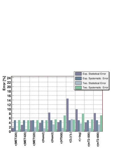
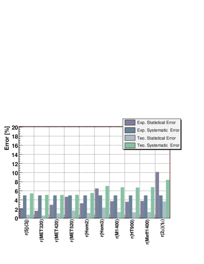
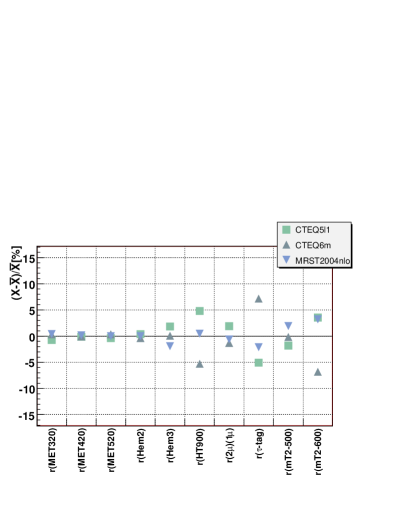
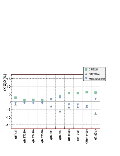
VII.4 CS6 vs LM2p, LM5, LM8 and CS4d

This is a complete example of how we could deduce the correct model, under the assumption of SUSY, based on how it fails to match with four incorrect SUSY models. We take CS6 as the “data” and compare it to LM2p, LM5, LM8 and CS4d.

With 100 pb^-1, the ratio r(mT2-500/300) is much smaller for the “data” than for LM2p, LM5, LM8 and CS4d, with significance 5.1, 4.6, 3.3 and 2.9$\sigma$ respectively. This indicates that the parent particle mass in the data model is quite a bit lighter than in model CS4d, which has the lightest squarks and gluinos of the four theory models.

To keep the overall data yield constant, we can contemplate two possible modifications of the spectrum in CS4d: either make the gluino lighter and the squarks heavier, or vice-versa.

The other striking result with 100 pb^-1 is that the “data” has only 1/4 as many events in the Muon20 box as the theory model LM8, and 1/3 as many as the theory model CS4d. At the same time, the “data” has nearly three times more $b$ tags in the Muon20 box than does LM8, a 6.5$\sigma$ discrepancy. With a little more data the same puzzling discrepancy turns up in the comparison with CS4d.

How to explain this? Recall that both models LM8 and CS4d produce a large number of $b$’s and $W$’s, and LM8 also has large numbers of $Z$’s. Events ending up in the Muon20 box have hard muons from either $W$/$Z$ decays or from energetic cascades with semileptonic $B$ decays in jets. If we removed all of the $W$’s and $Z$’s we would have many fewer events in the Muon20 box. However precisely in this case all of the events in the Muon20 box will have hard muons inside $b$ jets. This would then explain a high $b$ tagging rate in this box combined with a smaller overall count.

Already with 100 pb^-1 we have strong clues that the data model has a light gluino, heavy squarks, and that the gluino decays do not involve $W$’s, $Z$’s or sleptons. Table 19 shows that the “data” has only 59 $\tau$ tags per 1000 pb^-1; this gives a 6$\sigma$ deficiency in $\tau$ tags for the data relative to model LM2p after 1000 pb^-1. The lack of $\tau$ tags indicates we are not making a lot of $\tau$’s, but if we are not making either $W$’s or $\tau$’s then we are probably not making charginos from gluino decays. This suggests that the mass splitting between the gluino and the chargino is relatively small, and that the gluino has a three-body decay. A three-body decay mediated by a virtual chargino would imply more muons, so we a led to the three-body decay $\tilde{g}$$\rightarrow$ $q\bar{q}\tilde{\chi}_{1}^{0}$ mediated by a virtual squark.

Putting it all together (within the hypothesis of SUSY) leads to a model like CS6, with heavy squarks, a light gluino, and a compressed gaugino spectrum. Production is dominated by gluino pairs, and gluino decays are dominated by the three-body mode to $q\bar{q}\tilde{\chi}_{1}^{0}$. The only muons are from semileptonic $B$ decays.

This scenario also makes predictions that can be tested with more data. For example, the hemisphere counts should be quite symmetrical, since we are almost always producing a pair of the same particles with the same decays. Indeed this prediction is borne out with 1000 pb^-1, where both r(Hem2) and r(Hem3) are $>6\sigma$ smaller for CS6 than for LM8.

These hemisphere ratios also demonstrate the importance of the pdf uncertainties. Figures 23 and 24 show the breakdown of the uncertainties for some of the discriminating ratios with 1000 pb^-1 in the comparisons of CS6 “data” with models CS4d and LM8. For CS4d the r(Hem2) ratio, which discriminates at 4.6$\sigma$, is systematics limited, while the r(Hem3) ratio still has a rather large statistical uncertainty. For LM8 we notice that the theory systematic is the largest uncertainty for both r(Hem2) and r(Hem3).

These differences are explained by Figures 25 and 26, which show the spread in the values of the ratios as we vary the parton distribution functions used in the simulation. Note that the pdf spreads are model dependent: the spreads for the hemisphere ratios r(Hem2) and r(Hem3) are twice as large for LM8 as they are for CS4d. This explains why the total theory systematic for these ratios is larger for LM8 than for CS4d. However because of better statistics the hemisphere ratios appear to discriminate better for CS6 vs LM8 than they do for CS6 vs CS4d. The caveat is that the validity of this statement depends crucially on whether our estimates of the pdf uncertainties are at least roughly accurate.

VIII Summary of Group 2 results

Table 22 summarizes the results from the models of Group 2. There are 6 pairwise model comparisons. One model is taken as the simulated data, with the number of signal events scaled to either the 100 pb^-1 discovery data set or a 1000 pb^-1 follow-up. In our analysis we include the correct statistical uncertainty arising from the assumed 100 pb^-1 or 1000 pb^-1 of integrated luminosity in the “data” sample, as described in Section VI.B.

The most remarkable feature of these results is that we achieve greater than 4$\sigma$ discrimination of non-SUSY model LH2 from its SUSY look-alikes NM4 and CS7, already at the moment of discovery. With the larger 1000 pb^-1 data set, we achieve $>5\sigma$ discrimination in every case, for more than five distinct ratios per comparison. Thus even with small data sets we can both distinguish SUSY and non-SUSY explanations of the same excess and have multiple handles to inform us about key properties of the true model behind the data.

To see how this works in detail, let us take LH2 as our “data”. Suppose that we lived in a world where particle theorists believed that any missing energy signal has to be explained by SUSY (until recently we did in fact live in such a world). Then clever theorists might construct the SUSY model NM4 shown in Figure 6 as an explanation of the missing energy discovery.

Applying our look-alike analysis, however, one detects a problem already with 100 pb^-1. The $m_{T2}$ ratio r(mT2-500) (computed using the NM4 LSP mass) is three times larger for the “data” than for the SUSY model NM4, a nearly 5$\sigma$ discrepancy. As seen in Table 23, this is positively correlated with the $m_{T2}$ ratio r(mT2-500/300), which is more than twice as large for the “data” as for NM4, a 3$\sigma$ discrepancy, and uncorrelated with the jet multiplicity, which shows no significant difference.

These results strongly suggest that the true model underlying the “data” has heavier parent particles than does SUSY model NM4. However the SUSY enthusiast will be quite confused by this conclusion, since the kinematic ratio r(Meff1400) is more than two times greater for NM4 than it is for the “data”, a 3$\sigma$ discrepancy that seems to directly contradict our previous conclusion. A conservative SUSY enthusiast might choose to wait for more data, but this will only reinforce the confusion; with 1000 pb^-1 the ratio r(mT2-500/300) indicates with 8.5$\sigma$ significance that the NM4 squarks are too light, while r(Meff1400), r(M1400) and r(HT900) all indicate at $>5\sigma$ that SUSY NM4 events are too energetic!

At some point our SUSY enthusiast may decide to replace SUSY model NM4 with SUSY model CS7. This is a bright idea since the parent production in CS7 is all gluinos, instead of all squarks as in NM4, and the gluino kinematics are naturally softer then squark kinematics, for comparable masses. Thus, as seen in Table 24, CS7 matches both the kinematics and the overall yield of the “data” much better than NM4: even with 1000 pb^-1 r(Meff1400), r(M1400) and r(HT900) have no discrepancies as large as 3$\sigma$.

However our SUSY enthusiast still has serious problems. Table 24 shows that now the $E_{T}^{\rm{miss}}$ distributions are way off: even with 100 pb^-1 the ratio r(MET420) is more than twice as big for the “data” as for CS7, while r(MET520) is three times as big; these are both $>5\sigma$ discrepancies. Furthermore the jet multiplicities don’t match: the ratio r(4j)(3j) is almost twice as large for CS7 as for the “data”, a 4$\sigma$ discrepancy with 100 pb^-1.

Figures 27 and 28 demonstrate the robustness of these results, by showing the breakdown of the experimental and theoretical uncertainties for the relevant ratios. With the exception of r(4j)(3j), the uncertainties on all of the ratios that we have been discussing are completely dominated by the low statistics of our small “data” sample. Thus, for example, doubling the pdf uncertainties would not alter any of the conclusions reached above.

It is not obvious that our SUSY diehard can fix up a SUSY candidate to falsely explain the non-SUSY “data”, while surviving the scrutiny of our look-alike analysis. This applies even for small data sets on the order of a few hundred inverse picobarns. The key observation is that although SUSY models have many adjustable parameters, the number of adjustable parameters relevant to this look-alike analysis is small compared to the number of robust discriminators.

LH2 vs. NM4 [100 pb-1]
Variable	LH2	NM4	Separation
MET
r(mT2-500)	0.16	0.05	4.87
r(mT2-400)	0.44	0.21	4.84
r(mT2-300)	0.75	0.54	3.49
r(Meff1400)	0.11	0.25	2.99
r(mT2-500/300)	0.21	0.09	2.98
r(M1400)	0.07	0.19	2.69
r(mT2-400/300)	0.58	0.40	2.48
r(HT900)	0.13	0.24	2.34
r(MET420)	0.48	0.37	2.00
r(mT2-500/400)	0.36	0.22	1.47

Table 23: Best discriminating ratios in the MET box, with separations in units of $\sigma$, for the comparison of LH2 vs. NM4, taking LH2 as the “data”, assuming an integrated luminosity of 100 pb^-1.

LH2 vs. CS7 [100 pb-1]
Variable	LH2	CS7	Separation
MET
r(mT2-500)	0.27	0.08	6.68
r(MET420)	0.48	0.20	6.49
r(MET520)	0.21	0.07	5.06
r(MET320)	0.78	0.53	4.29
r(mT2-500/300)	0.32	0.12	4.24
r(4j)(3j)	0.36	0.61	4.04
r(mT2-400)	0.63	0.40	4.00
r(mT2-300)	0.85	0.62	3.55
r(mT2-500/400)	0.43	0.19	3.52
r(Hem1)	0.79	0.63	2.59

Table 24: Best discriminating ratios in the MET box, with separations in units of $\sigma$, for the comparison of LH2 vs. CS7, taking LH2 as the “data”, assuming an integrated luminosity of 100 pb^-1.

Figure 27: Breakdown of estimated uncertainties for discriminating ratios with 100 pb^-1, in the comparison of look-alike models LH2 and NM4, with LH2 treated as the “data”.

Figure 28: Breakdown of estimated uncertainties for discriminating ratios with 100 pb^-1, in the comparison of look-alike models LH2 and CS7, with LH2 treated as the “data”.

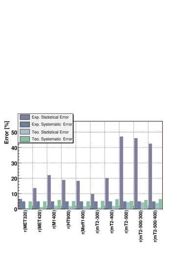
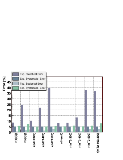
IX Discussion and outlook

We have presented a concrete strategy for determining the underlying theory model of an early missing energy discovery at the LHC. Applying this look-alike analysis to a realistic simulation, we were able to distinguish a non-SUSY model from its SUSY look-alikes essentially at the moment of discovery, with little more than 100 pb^-1 of integrated luminosity. In 23 of 26 pairwise comparisons, mostly SUSY with SUSY, we were able to discriminate look-alikes at better than 5$\sigma$ significance with at least one robust observable and 1000 pb^-1 or less of integrated luminosity. Even in the three cases with the worst discrimination we found strong hints of the key properties of the underlying model; these would be confirmed with more data and/or by our improving the look-alike analysis.

One surprise of our study (at least to us) was the sensitivity and robustness of the ratios based on the stransverse mass $m_{T2}$. Keep in mind that we did not apply the $m_{T2}$ distributions to their originally intended use i.e. extracting masses from endpoints and kinks, and we applied our $m_{T2}$ ratios to data sets 100 times smaller than used in previous studies. Nevertheless we found that the $m_{T2}$ ratios are among our best discriminators. One of the most important features of the $m_{T2}$ ratios is that to first approximation they do not depend on the spins of the parent particles. Since ratios based on more traditional kinematic distributions like $H_{T}$ and $M_{\rm eff}$ have a large dependence on the spins of the parent particles, comparing $m_{T2}$ ratios to these ratios is a powerful discriminator for spin.

Our main goal in this study was to develop a look-alike analysis for missing energy that can be successfully applied to the LHC data in the first year of physics running. The crucial properties of such an analysis are realism, robustness, validation and sensitivity. We briefly summarize where we stand with respect to establishing these properties.

Realism

We have employed state-of-the-art event generation for the missing energy signals, but only at leading order in each subprocess. In the next phase we include the possibility of extra high $E_{T}$ jets at the matrix element level. We are performing this study within the CMS collaboration and hence replace our fast simulation with the full CMS detector simulation. This also allows us to include the Standard Model backgrounds in the full analysis, replacing the background subtraction assumed here.

Robustness

Our analysis is already quite robust against disappointments in the performance of the LHC detectors during the first physics run. We have assumed a minimal palette of reconstructed objects and triggers. Because our analysis uses only ratios of correlated inclusive counts, there is a large cancellation of theoretical and experimental uncertainties, and we can make simple apples–with–apples comparisons between different observables.

Despite the fact that we are considering small data sets, we have not employed any multivariate statistical methods. As mentioned earlier such methods are left for the era of demonstrated understanding of the correlations between observables. By dispensing with these methods we lose sensitivity but gain a cleaner more robust analysis.

We gain additional robustness from the physics redundancy built into our choice of correlated observables. For example, jet multiplicity is correlated with track counts in the cones, and sometimes with the ratios of $m_{T2}$ counts to total number of events in the box. The hemisphere ratios are correlated with the difference counts in the cones. Muon counting is correlated with $b$ tagging. The four trigger boxes provide us with four complete sets of ratios, allowing further comparisons and cross-checks.

Our main deficiency in robustness is the limited number of theory models simulated for this study. In the next phase we are including a much larger number and variety of models.

A possible approach to expanding this analysis is to apply the idea of OSETs ArkaniHamed:2007fw , as a strategy for effectively sampling the entire theory space. A disadvantage of this approach is that, by definition, we give up our spin sensitivity and more generally any discrimination based on details of the matrix elements.

Validation

No studies performed to date of the LHC phenomenology of any BSM theory have adequately validated uncertainties. The experimental uncertainties cannot be sufficiently validated until we have LHC data. The theoretical uncertainties could be validated sooner, but this will require many more detailed studies adhering to at least the degree of realism attempted here.

In the next phase of this analysis (currently being performed within the CMS collaboration) we are validating the Standard Model backgrounds of the inclusive missing energy signature using the CMS full simulation framework. This, among other things, is allowing us to compute the backgrounds in each of our trigger boxes and study the effect of varying the selection criteria, e.g. relaxing or modifying the ILV.

The full detector simulation itself needs to be validated against real LHC data, using these same Standard Model processes as benchmarks. Similar comments apply to the parton distribution functions. In both cases we need to develop a more sophisticated parametrization of the uncertainties.

The event generation chains used in our study, while state-of-the-art, have not been adequately validated; we have performed several cross-validation checks and obtained significant discrepancies. This is an important task for the entire LHC theory community.

Sensitivity

We have demonstrated the importance of being able to obtain subsamples of the discovery data set enriched in $\tau$’s and $b$’s. To do this successfully will require a different approach to flavor tagging in the early LHC running, an approach that emphasizes robustness and fast validation over efficiency and purity. It seems likely that a dedicated effort could achieve results as good as our preliminary study, and possibly much better.

We have seen that one of the virtues of the $m_{T2}$ ratios is sensitivity to the number of weakly interacting particles in the final state. It is important to study this further, along with the potential to extract estimates of the masses of parent particles and the LSP from small data sets.

Dark matter at 100 pb^-1

We have demonstrated a concrete strategic solution to the LHC Inverse Problem applicable under realistic conditions to early physics running at the LHC. Since the missing energy signature is motivated by the existence of dark matter, we should also address what might be called the Dark Matter Inverse Problem: given a missing energy discovery at the LHC, what can we learn about dark matter and the cosmological events that produced it? This problem has not been addressed at all for the 100 pb^-1 era of LHC running. Given an early missing energy discovery at the LHC, this problem will become one of the most interesting questions in particle physics, especially tied in to results from the ongoing direct and indirect dark matter searches.

LM5 vs. CS4d [100 pb-1]
Variable	LM5	CS4d	Separation
MET
r(HT900)	0.38	0.24	3.59
r(Meff1400)	0.32	0.21	3.15
r(MET520)	0.28	0.19	3.12
DiJet
r(DiJet)	0.22	0.15	2.37
r(MET520)	0.28	0.23	0.56
r(Hem2)	0.27	0.32	0.51
TriJet
r(TriJet)	0.22	0.17	1.89
r(Meff1400)	0.65	0.59	0.62
r(HT900)	0.73	0.67	0.59
Muon20
r(HT900)	0.35	0.25	1.17
r(mT2-300)	0.27	0.36	1.00
r(mT2-400)	0.26	0.34	0.93

Table 25: Largest separation (in units of $\sigma$) for the comparison of LM5 vs. CS4d (error on CS4d) assuming an integrated luminosity of 100 pb^-1.

LM5 vs. CS4d [100 pb-1]
Variable	LM5	CS4d	Separation
MET
r(HT900)	0.38	0.24	3.59
r(Meff1400)	0.32	0.21	3.15
r(MET520)	0.28	0.19	3.12
r(mT2-600/300)	0.29	0.17	2.83
r(mT2-600/400)	0.31	0.18	2.82
r(mT2-600/500)	0.46	0.30	2.22
r(MET420)	0.49	0.40	2.14
r(mT2-300)	0.36	0.45	1.98
r(mT2-400)	0.34	0.43	1.87
r(mT2-600)	0.11	0.08	1.47

Table 26: Largest separation (in units of $\sigma$) for the comparison of LM5 vs. CS4d (error on CS4d) assuming an integrated luminosity of 100 pb^-1.

LM5 vs. CS4d [1000 pb-1]
Variable	LM5	CS4d	Separation
MET
r(MET520)	0.28	0.19	7.07
r(HT900)	0.38	0.24	6.41
r(mT2-600/400)	0.31	0.18	6.10
DiJet
r(DiJet)	0.22	0.15	4.80
r(mT2-600/300)	0.29	0.15	2.69
r(mT2-600/400)	0.30	0.16	2.69
TriJet
r(TriJet)	0.22	0.17	3.50
r(MET520)	0.28	0.24	1.31
r(Meff1400)	0.65	0.59	1.29
Muon20
r(mT2-600/300)	0.23	0.13	3.04
r(mT2-600/400)	0.25	0.14	2.98
r(HT900)	0.35	0.25	2.63

Table 27: Best discriminating ratios in each trigger box, with separations in units of $\sigma$, for the comparison of LM5 vs. CS4d, taking LM5 as the “data”, assuming an integrated luminosity of 1000 pb^-1.

LM5 vs. CS4d [1000 pb-1]
Variable	LM5	CS4d	Separation
MET
r(MET520)	0.28	0.19	7.07
r(HT900)	0.38	0.24	6.41
r(mT2-600/400)	0.31	0.18	6.10
r(mT2-600/300)	0.29	0.17	6.04
r(Meff1400)	0.32	0.21	5.94
r(mT2-600/500)	0.46	0.30	4.88
r(MET420)	0.49	0.40	3.82
r(mT2-600)	0.11	0.08	3.52
r(mT2-300)	0.36	0.45	3.12
r(mT2-400)	0.34	0.43	3.02

Table 28: Best discriminating ratios in the MET box, with separations in units of $\sigma$, for the comparison of LM5 vs. CS4d, taking LM5 as the “data”, assuming an integrated luminosity of 1000 pb^-1.

LM2p vs. LM5 [100 pb-1]
Variable	LM2p	LM5	Separation
MET
r(5j)(3j)	0.33	0.40	1.64
r(mT2-300)	0.41	0.34	1.44
r(mT2-400)	0.30	0.25	1.34
r(4j)(3j)	0.64	0.69	1.18
r($\tau$-tag)	0.07	0.05	1.17
r(10t-c45)	0.30	0.36	1.14
r(10t-c30)	0.16	0.20	1.13
r(10t-c75)	0.48	0.53	1.07
r(10t-c60)	0.41	0.47	1.07
r(mT2-500)	0.16	0.13	1.05

Table 29: Best discriminating ratios in the MET box, with separations in units of $\sigma$, for the comparison of LM2p vs. LM5, taking LM2p as the “data”, assuming an integrated luminosity of 100 pb^-1.

Figure 29: Breakdown of estimated uncertainties for discriminating ratios with 100 pb^-1, in the comparison of look-alike models LM2p and LM5, with LM2p treated as the “data”.

Figure 30: Pdf spreads for discriminating ratios with 100 pb^-1, in the comparison of look-alike models LM2p and LM5, with LM2p treated as the “data”.

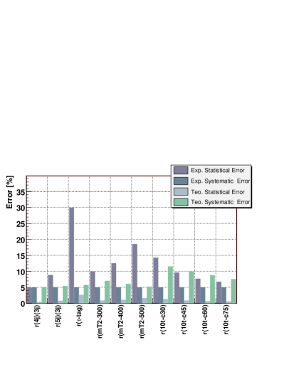
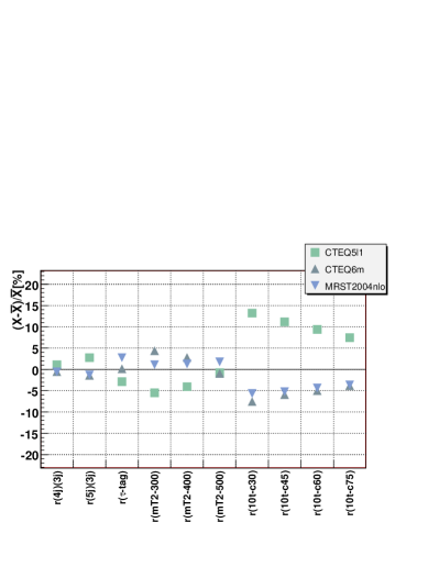
Acknowledgments

The authors are grateful to Keith Ellis, Gordon Kane, Filip Moortgat, Stephen Mrenna, Luc Pape, Tilman Plehn, Chris Quigg, Sezen Sekmen, Phillip Schuster, Peter Skands and Natalia Toro for useful discussions. JL and MS acknowledge the Michigan Center for Theoretical Physics for hospitality during the concluding phase of this work; JH similarly acknowledges the Kavli Institute for Theoretical Physics. Fermilab is operated by the Fermi Research Alliance LLC under contract DE-AC02-07CH11359 with the U.S. Dept. of Energy. Research at Argonne National Laboratory Division is supported by the U.S. Dept. of Energy under contract DE-AC02-06CH11357.

Figure 31: Pulls of the best discriminating ratios with 100 pb^-1, in the comparison of look-alike models LM2p and LM5, with LM2p treated as the “data”.

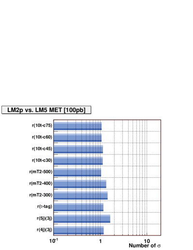
LM2p vs. LM5 [1000 pb-1]
Variable	LM2p	LM5	Separation
MET
r($\tau$-tag)	0.07	0.05	3.14
r(5j)(3j)	0.33	0.40	2.77
r(mT2-400)	0.30	0.25	2.56
r(mT2-500)	0.16	0.13	2.53
r(mT2-300)	0.41	0.34	2.27
r(10t-c30)	0.16	0.20	1.67
r(MET520)	0.31	0.28	1.67
r(20t-c45)	0.07	0.09	1.61
r(10tdiff-c30)	0.14	0.16	1.61
r(4j)(3j)	0.64	0.69	1.56

Table 30: Best discriminating ratios in the MET box, with separations in units of $\sigma$, for the comparison of LM2p vs. LM5, taking LM2p as the “data”, assuming an integrated luminosity of 1000 pb^-1.

CS4d vs. LM8 [100 pb-1]
Variable	CS4d	LM8	Separation
MET
r(5j)(3j)	0.40	0.54	2.83
r(mT2-300)	0.41	0.32	2.14
r(4j)(3j)	0.70	0.81	2.11
r(10t-c30)	0.20	0.28	1.93
r(20t-c60)	0.16	0.23	1.78
r(20t-c45)	0.08	0.13	1.73
r(10t-c30)(10t-c90)	0.34	0.43	1.72
r(10t-c45)	0.36	0.46	1.70
r(30t-c90)	0.11	0.17	1.68
r(Meff1400)	0.21	0.28	1.65

Table 31: Best discriminating ratios in the MET box, with separations in units of $\sigma$, for the comparison of CS4d vs. LM8, taking CS4d as the “data”, assuming an integrated luminosity of 100 pb^-1.

CS4d vs. LM8 [1000 pb-1]
Variable	CS4d	LM8	Separation
MET
r(5j)(3j)	0.40	0.54	4.21
r(10tdiff-c30)	0.15	0.20	3.63
r(Hem3)	0.07	0.11	3.58
r(mT2-300)	0.41	0.32	3.43
r(mT2-400)	0.25	0.20	3.24
r(20t-c30)	0.02	0.04	3.09
r(20tdiff-c45)	0.06	0.08	3.05
r(20tdiff-c60)	0.12	0.16	3.04
r(20t-c45)	0.08	0.13	3.03
r(10t-c30)(10t-c90)	0.34	0.43	2.95

Table 32: Best discriminating ratios in the MET box, with separations in units of $\sigma$, for the comparison of CS4d vs. LM8, taking CS4d as the “data”, assuming an integrated luminosity of 1000 pb^-1.

Figure 32: Breakdown of estimated uncertainties for discriminating ratios with 100 pb^-1, in the comparison of look-alike models CS4d and LM8, with CS4d treated as the “data”.

Figure 33: Breakdown of estimated uncertainties for discriminating ratios with 100 pb^-1, in the comparison of look-alike models CS4d and LM8, with CS4d treated as the “data”.

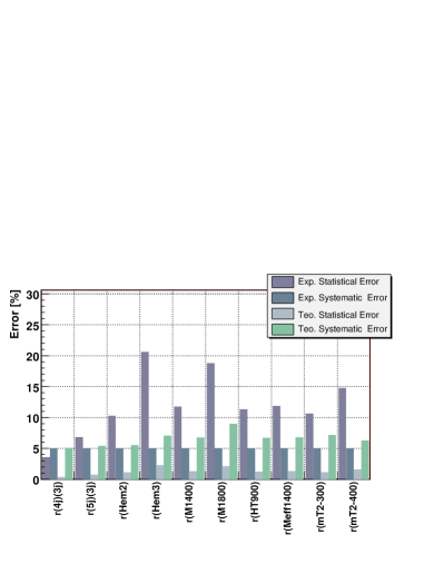
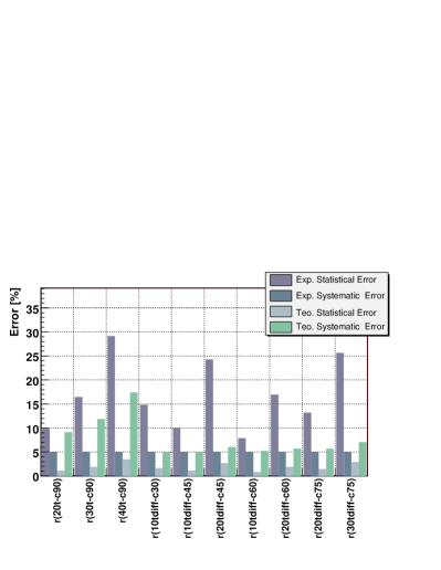
CS6 vs. LM2p [100 pb-1]
Variable	CS6	LM2p	Separation
MET
r(MET420)	0.22	0.53	6.99
r(MET520)	0.09	0.31	6.10
r(mT2-500/300)	0.08	0.39	5.14
DiJet
r(DiJet)	0.11	0.21	3.04
r(5j)(3j)	0.54	0.32	3.00
r(4j)(3j)	0.83	0.62	2.56
TriJet
r(MET420)	0.29	0.53	2.96
r(MET320)	0.55	0.77	2.84
r(HT900)	0.57	0.75	2.46
Muon20
r($b$-tag)	0.74	0.36	4.25
r(Muon20)	0.06	0.14	3.14
r(MET420)	0.23	0.48	2.55

Table 33: Best discriminating ratios in each trigger box, with separations in units of $\sigma$, for the comparison of CS6 vs. LM2p, taking CS6 as the “data”, assuming an integrated luminosity of 100 pb^-1.

CS6 vs. LM2p [100 pb-1]
Variable	CS6	LM2p	Separation
MET
r(MET420)	0.22	0.53	6.99
r(MET520)	0.09	0.31	6.10
r(mT2-500/300)	0.08	0.39	5.14
r(mT2-500/400)	0.17	0.54	5.11
r(MET320)	0.54	0.78	4.93
r(HT900)	0.18	0.38	4.80
r(mT2-500)	0.03	0.16	4.56
r(Meff1400)	0.16	0.32	3.91
r(mT2-400/300)	0.49	0.73	3.88
r(mT2-400/300)	0.49	0.73	3.88

Table 34: Best discriminating ratios in the MET box, with separations in units of $\sigma$, for the comparison of CS6 vs. LM2p, taking CS6 as the “data”, assuming an integrated luminosity of 100 pb^-1.

Figure 34: Breakdown of estimated uncertainties for discriminating ratios with 100 pb^-1, in the comparison of look-alike models CS6 and LM2p, with CS6 treated as the “data”.

Figure 35: Comparison of the $m_{T2}$ distribution of the CS6 “data” (solid red line) to that of the theory model LM2p (dashed blue line) for 100 pb^-1. Here $m_{T2}$ is computed using the LSP mass of the theory model LM2p.

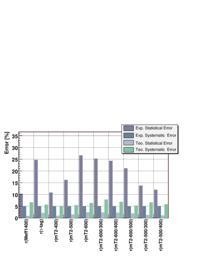
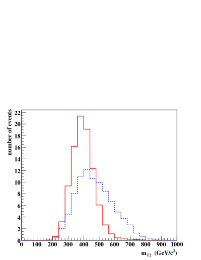
Appendix A Detailed results for Group 1

A.1 LM5 vs CS4d

This comparison is described in section VII.1. We treat model LM5 as the data and CS4d as the theory model. For 100 pb^-1 of integrated luminosity, Table 25 shows the three best discriminating ratios as defined in each of the trigger boxes: MET, DiJet, TriJet and Muon20. Table 26 shows the ten best discriminating ratios in the MET box. The separation in units of $\sigma$ is computed from the total estimated theoretical and experimental uncertainties as described in section VI.

The same information for 1000 pb^-1 is shown in Tables 27 and 28. The notation r(DiJet), r(TriJet) and r(Muon20) denotes the ratio of the number of events in that box with the number of events in the MET box. Since (plus or minus about one event in 1000 pb^-1) the DiJet, TriJet and Muon20 boxes are subsamples of the MET box, these are ratios of inclusive counts.

A.2 LM2p vs LM5

This comparison is described in section VII.2. We treat model LM2p as the data and LM5 as the theory model. For 100 pb^-1, the ten best discriminating ratios are listed in Table 29 and the pulls are displayed in Figure 31. While the $\tau$ tag ratio is not discriminating well, Figure 29 shows that this is due entirely to poor statistics in this small simulated data sample: the experimental statistical uncertainty is 30%, compared to experimental and theory systematics both estimated at around 5%. The small theory statistical uncertainty shown is the error from the finite Monte Carlo statistics in simulating the theory model. Table 30 shows the improvement in the discriminating power of r($\tau$-tag) with 1000 pb^-1, due to the reduction in the experimental statistical uncertainty. Note that in this difficult case no other ratio discriminates with better than 3$\sigma$ significance.

In Figure 29 one also notices large differences in the relative size of the theory systematics for the different ratios. These are due to large differences in the spread of values when we vary the parton distribution functions used in the simulation, as shown in Figure 30. Notice that the pdf spreads vary from less than 5% for the jet multiplicity ratio r(4j)(3j) to greater than 20% for the cone track count ratio r(10t-c30).

This is an important generic feature of our results. We find the pdf uncertainties to be process dependent and thus model dependent. We find also that the relative pdf uncertainties for different ratios in the same model vary by factors as large as 4 or 5.

A.3 CS4d vs LM8

This comparison is described in section VII.3. We treat model CS4d as the data and LM8 as the theory model. Tables 31 and 32 show the ten best discriminating ratios for 100 pb^-1 and 1000 pb^-1 respectively. We observe that the best discriminator with 100 pb^-1, the jet multiplicity ratio r(5j)(3j), remains the best with 1000 pb^-1. However the second and third best dsicriminators with 1000 pb^-1, r(10tdiff-c30) and r(Hem3), are not even among the top ten best with 100 pb^-1.

These again are generic features of our results. Figures 32 and 33 show that with 100 pb^-1 r(5j)(3j) already has a statistical uncertainty comparable to the estimated systematics, while many other ratios still have large 15 to 20% statistical uncertainties. This includes r(10tdiff-c30) and r(Hem3), ratios that are sensitive to what fraction of events have large hemisphere differences in object counts or track counts. Thus qualitatively new features of the events emerge automatically as good discriminators as the integrated luminosity goes up, without changing the design of the look-alike analysis.

A.4 CS6 vs LM2p, LM5, LM8 and CS4d

This comparison is described in section VII.4. We treat model CS6 as the data and compare to theory models LM2p, LM5, LM8 and CS4d. Tables 33 and 34 show the best discriminating ratios for the comparison of LM2p to the CS6 “data” with 100 pb^-1. We see that two $E_{T}^{\rm{miss}}$ ratios and two $m_{T2}$ ratios already discriminate at better than 5$\sigma$.

Figure 34 shows the breakdown of the uncertainites for some of the ratios in the this comparison. Observe that the kinematic ratio r(Meff1400) has a smaller experimental statistical uncertainty than do the $m_{T2}$ ratios r(mT2-500/300) and r(mT2-500/400); nevertheless Table 34 shows that r(Meff1400) is a worse discriminator.

This is a generic feature of our results. The distributions in $M_{\rm eff}$ are rather broad, whereas the $m_{T2}$ distributions are steeply falling as one approaches the endpoint region. As seen in Figure 35, when the parent particle mass differences are large, $m_{T2}$ is an intrinsically good discriminator even for quite small data samples within very modest resolutions.

Tables 35 and 36 show the best discriminating ratios for the comparison of LM8 ans CS4d to the CS6 “data” with 100 pb^-1. These results show the importance of the ratios in the Muon20 box.

CS6 vs. LM8 [100 pb-1]
Variable	CS6	LM8	Separation
MET
r(MET420)	0.22	0.39	4.03
r(Hem2)	0.19	0.34	3.60
r(MET520)	0.09	0.20	3.45
DiJet
r(DiJet)	0.11	0.18	2.21
r(Hem2)	0.28	0.35	0.87
r(MET320)	0.59	0.66	0.86
TriJet
r(Meff1400)	0.50	0.64	1.58
r(HT900)	0.57	0.68	1.35
r(MET320)	0.55	0.66	1.21
Muon20
r($b$-tag)	0.74	0.29	6.45
r(Muon20)	0.06	0.24	5.19
r(MET420)	0.23	0.36	1.78

Table 35: Best discriminating ratios in each trigger box, with separations in units of $\sigma$, for the comparison of CS6 vs. LM8, taking CS6 as the “data”, assuming an integrated luminosity of 100 pb^-1.

CS6 vs. CS4d [100 pb-1]
Variable	CS6	CS4d	Separation
MET
r(MET420)	0.22	0.40	4.25
r(MET320)	0.54	0.70	3.26
r(MET520)	0.09	0.19	3.15
DiJet
r(5j)(3j)	0.54	0.39	1.53
r(DiJet)	0.11	0.15	1.42
r(4j)(3j)	0.83	0.69	1.41
TriJet
r(MET320)	0.55	0.70	1.63
r(MET420)	0.29	0.43	1.53
r(HT900)	0.57	0.67	1.17
Muon20
r(Muon20)	0.06	0.18	3.95
r(MET320)	0.54	0.69	1.73
r(MET420)	0.23	0.37	1.59

Table 36: Best discriminating ratios in each trigger box, with separations in units of $\sigma$, for the comparison of CS6 vs. CS4d, taking CS6 as the “data”, assuming an integrated luminosity of 100 pb^-1.

LH2 vs. NM4 [1000 pb-1]
Variable	LH2	NM4	Separation
MET
r(mT2-500)	0.16	0.05	14.11
r(mT2-400)	0.44	0.21	11.13
r(mT2-500/300)	0.21	0.09	8.52
DiJet
r(mT2-400)	0.32	0.12	7.89
r(mT2-300)	0.64	0.32	7.79
r(DiJet)	0.11	0.22	5.94
TriJet
r(mT2-300)	0.62	0.19	10.96
r(mT2-400)	0.34	0.07	10.91
r(TriJet)	0.06	0.15	5.94
Muon20
r(mT2-400)	0.38	0.14	5.03
r(mT2-300)	0.72	0.42	4.30
r(Meff1400)	0.10	0.34	3.50

Table 37: Best discriminating ratios in each trigger box, with separations in units of $\sigma$, for the comparison of LH2 vs. NM4, taking LH2 as the “data”, assuming an integrated luminosity of 1000 pb^-1.

LH2 vs. NM4 [1000 pb-1]
Variable	LH2	NM4	Separation
MET
r(mT2-500)	0.16	0.05	14.11
r(mT2-400)	0.44	0.21	11.13
r(mT2-500/300)	0.21	0.09	8.52
r(Meff1400)	0.11	0.25	7.24
r(M1400)	0.07	0.19	6.57
r(mT2-300)	0.75	0.54	6.26
r(mT2-400/300)	0.58	0.40	5.77
r(HT900)	0.13	0.24	5.67
r(M1800)	0.02	0.07	4.82
r(MET420)	0.48	0.37	4.32

Table 38: Best discriminating ratios in the MET box, with separations in units of $\sigma$, for the comparison of LH2 vs. NM4, taking LH2 as the “data”, assuming an integrated luminosity of 1000 pb^-1.

LH2 vs. CS7 [1000 pb-1]
Variable	LH2	CS7	Separation
MET
r(mT2-500)	0.27	0.08	18.87
r(MET420)	0.48	0.20	16.73
r(MET520)	0.21	0.07	14.49
DiJet
r(4j)(3j)	0.20	0.67	7.30
r(mT2-300)	0.72	0.31	6.73
r(mT2-400)	0.53	0.22	6.26
TriJet
r(mT2-500)	0.20	0.04	8.83
r(mT2-300)	0.68	0.32	7.43
r(mT2-400)	0.53	0.22	7.18
Muon20
r(mT2-300)	0.84	0.35	1.57
r(mT2-400)	0.60	0.24	1.32

Table 39: Best discriminating ratios in each trigger box, with separations in units of $\sigma$, for the comparison of LH2 vs. CS7, taking LH2 as the “data”, assuming an integrated luminosity of 1000 pb^-1.

LH2 vs. CS7 [1000 pb-1]
Variable	LH2	CS7	Separation
MET
r(mT2-500)	0.27	0.08	18.87
r(MET420)	0.48	0.20	16.73
r(MET520)	0.21	0.07	14.49
r(mT2-600)	0.05	0.01	14.11
r(mT2-500/300)	0.32	0.12	11.17
r(mT2-500/400)	0.43	0.19	9.77
r(mT2-600/300)	0.06	0.01	9.77
r(mT2-400)	0.63	0.40	8.46
r(MET320)	0.78	0.53	8.17

Table 40: Best discriminating ratios in the MET box, with separations in units of $\sigma$, for the comparison of LH2 vs. CS7, taking LH2 as the “data”, assuming an integrated luminosity of 1000 pb^-1.

Appendix B Detailed results for Group 2

B.1 LH2 vs NM4 and CS7

This comparison is described in section VIII. We treat the little Higgs model LH2 as the data and compare to SUSY models NM4 and CS7. Tables 37-40 show the best discriminating ratios for the comparison of NM4 and CS7 to the LH2 “data” with 1000 pb^-1.

With the better statistics of 1000 pb^-1, Table 38 illustrates even more clearly the conundrum discussed in section  VIII. The $m_{T2}$ ratio r(mT2-500/300) shows unquestionably that the parent particle masses in model NM4 are too small to fit the “data”. The $E_{T}^{\rm{miss}}$ distribution of NM4 also appears to be too soft, with 4.3$\sigma$ significance. However the kinematic distributions for NM4 represented by r(Meff1400), r(M1400) and r(HT900) are all too hard, with $>5\sigma$ significance.

The other impressive feature of these tables is that with 1000 pb^-1 we acquire several highly discriminating ratios in the DiJet and TriJet boxes. With real data this would provide an impressive redundancy of cross-checks, still within the original design of our look-alike analysis.

The large number of independent highly discriminating robust ratios seen here provide a powerful tool to resolve SUSY look-alikes from non-SUSY look-alikes.

Appendix C Comparison of squark production with heavy quark production

C.1 smuon production versus muon production

Let’s compare the QED processes $e^{+}e^{-}\rightarrow\mu^{+}\mu^{-}$ and $e^{+}e^{-}\rightarrow\tilde{\mu}_{R}\bar{\tilde{\mu}}_{R}$. We will use the conventions and notation of Peskin and Schroeder (PS) Peskin:1995ev , and work in the approximation that the electron and positron are massless. In this notation $p$ and $p^{\prime}$ denote the incoming 4-momenta of the electron and positron, while $k$ and $k^{\prime}$ denote the outgoing 4-momenta of the muons or smuons. The photon 4-momentum is denoted by $q=p+p^{\prime}$. We will use $m$ interchangably to denote the mass of the muon or smuon, assuming them (in this pedagogical example) to be degenerate.

The leading order QED matrix element for $e^{+}e^{-}\rightarrow\mu^{+}\mu^{-}$ is

$$\bar{v}^{s^{\prime}}(p^{\prime})(-ie\gamma^{\mu})u^{s}(p)\left(\frac{-i}{q^{2}}\right)\bar{u}^{r}(k)(-ie\gamma_{\mu})v^{r^{\prime}}(k^{\prime})$$ (10)

The corresponding matrix element for $e^{+}e^{-}\rightarrow\tilde{\mu}_{R}\bar{\tilde{\mu}}_{R}$ is

$$\bar{v}^{s^{\prime}}(p^{\prime})(-ie\gamma^{\mu})u^{s}(p)\left(\frac{-i}{q^{2}}\right)(-ie(k_{\mu}-k^{\prime}_{\mu}))$$ (11)

In each case, we compute the squared matrix element, averaging over the spins of the electrons. For $e^{+}e^{-}\rightarrow\mu^{+}\mu^{-}$ we also sum over the spins of the muons, thus

$$\textstyle{\frac{1}{4}\sum_{s,s^{\prime},r,r^{\prime}}|{\cal M}(s,s^{\prime},r,r^{\prime})|^{2}=\frac{e^{4}}{4q^{4}}{\rm tr}\left[\not{\hbox{\kern-2.0ptp}}^{\prime}\gamma^{\mu}\not{\hbox{\kern-2.0ptp}}\gamma^{\nu}\right]}$$

$$\textstyle{\times{\rm tr}\left[(\not{\hbox{\kern-2.0ptk}}+m)\gamma_{\mu}(\not{\hbox{\kern-2.0ptk}}^{\prime}-m)\gamma_{\nu}\right]}\;,$$ (12)

while for $e^{+}e^{-}\rightarrow\tilde{\mu}_{R}\bar{\tilde{\mu}}_{R}$ we have

$$\textstyle{\frac{1}{4}\sum_{s,s^{\prime}}|{\cal M}(s,s^{\prime})|^{2}=}$$

$$\hskip 20.0pt\textstyle{\frac{e^{4}}{4q^{4}}{\rm tr}\left[\not{\hbox{\kern-2.0ptp}}^{\prime}\gamma^{\mu}(k_{\mu}-k^{\prime}_{\mu})\not{\hbox{\kern-2.0ptp}}\gamma^{\nu}(k_{\nu}-k^{\prime}_{\nu})\right]}\;.$$ (13)

From now on we will follow the convention of Ellis, Stirling and Webber (ESW) Ellis:1991qj and use a barred summation to denote the average over initial spins and sum over final spins (if any). Thus performing the traces (C.1) becomes

$$\textstyle{\overline{\sum}|{\cal M}|^{2}=\frac{8e^{4}}{q^{4}}\left[(p\cdot k)(p^{\prime}\cdot k^{\prime})+(p\cdot k^{\prime})(p^{\prime}\cdot k)+m^{2}(p\cdot p^{\prime})\right]}$$ (14)

while (C.1) becomes

$$\textstyle{\overline{\sum}|{\cal M}|^{2}=\frac{2e^{4}}{q^{4}}\bigl{[}(p\cdot p^{\prime})(k\cdot k^{\prime})-(p\cdot k)(p^{\prime}\cdot k^{\prime})-(p\cdot k^{\prime})(p^{\prime}\cdot k)}$$

$$\hskip 10.0pt\textstyle{+(p\cdot k)(p^{\prime}\cdot k)+(p\cdot k^{\prime})(p^{\prime}\cdot k^{\prime})-m^{2}(p\cdot p^{\prime})\bigr{]}}\;.$$ (15)

The kinematics of both cases are identical; in the center of mass frame:

$$p\cdot p^{\prime} =\displaystyle{\frac{s}{2},}\quad k\cdot k^{\prime} =\quad\frac{s}{4}(1+\beta^{2})\,;$$

$$p\cdot k =\quad p^{\prime}\cdot k^{\prime} =\quad\frac{s}{4}(1-\beta\,{\rm cos}\,\theta)\,;$$ (16)

$$p\cdot k^{\prime} =\quad p^{\prime}\cdot k =\quad\frac{s}{4}(1+\beta\,{\rm cos}\,\theta)\,,$$

where $\theta$ is the polar angle of the final state muon or smuon, and

$$\textstyle{\beta\equiv\sqrt{1-\frac{4m^{2}}{s}}}\;.$$ (17)

Substituting, (14) becomes

$$\textstyle{\overline{\sum}|{\cal M}|^{2}=e^{4}\left[2-\beta^{2}(1-{\rm cos}^{2}\theta)\right]}\,,$$ (18)

and (C.1) becomes

$$\textstyle{\overline{\sum}|{\cal M}|^{2}=\frac{e^{4}}{2}\beta^{2}(1-{\rm cos}^{2}\theta)}\,.$$ (19)

Thus the differential cross section for $e^{+}e^{-}\rightarrow\mu^{+}\mu^{-}$ at leading order in QED is

$$\frac{d\sigma}{d({\rm cos}\,\theta)}=\frac{\pi\alpha^{2}}{2s}\beta\,\left[2-\beta^{2}(1-{\rm cos}^{2}\theta)\right]\,,$$ (20)

while for $e^{+}e^{-}\rightarrow\tilde{\mu}_{R}\bar{\tilde{\mu}}_{R}$ we get

$$\frac{d\sigma}{d({\rm cos}\,\theta)}=\frac{\pi\alpha^{2}}{4s}\beta^{3}\,(1-{\rm cos}^{2}\theta)\,,$$ (21)

agreeing with Farrar and Fayet Farrar:1980uy .

Since a Dirac muon has two complex scalar superpartners, $\tilde{\mu}_{R}$ and $\tilde{\mu}_{L}$, from now on we will write the combined cross section for $e^{+}e^{-}\rightarrow\tilde{\mu}_{R}\bar{\tilde{\mu}}_{R}+\tilde{\mu}_{L}\bar{\tilde{\mu}}_{L}$, which is just twice the expression in (21). Thus we have the total cross sections:

$$\sigma(e^{+}e^{-}\rightarrow\mu^{+}\mu^{-}) = \frac{2\pi\alpha^{2}}{3s}\beta(3-\beta^{2})\,;$$

$$\sigma(e^{+}e^{-}\rightarrow\tilde{\mu}_{R}\bar{\tilde{\mu}}_{R}+\tilde{\mu}_{L}\bar{\tilde{\mu}}_{L}) = \frac{2\pi\alpha^{2}}{3s}\beta^{3}\,.$$ (22)

In the high energy limit $\beta\rightarrow 1$, the leading order muon pair cross section is exactly twice the smuon pair cross section, as noted for example in Choi:2006mr .

C.2 $\mathbf{q\bar{q}\rightarrow Q\bar{Q}}$ versus $\mathbf{q\bar{q}\rightarrow\tilde{q}\bar{\tilde{q}}}$

From these formulae it is easy to obtain the leading order cross sections for hadroproduction of heavy quarks/squarks from light $q\bar{q}$ initial parton states. First we introduce a kinematic notation more suitable for hadroproduction. The subprocess Mandelstam invariants are given by

$$\hat{t} = m^{2}-\frac{\hat{s}}{2}(1-\beta\,{\rm cos}\,\theta)\;;$$

$$\hat{u} = m^{2}-\frac{\hat{s}}{2}(1+\beta\,{\rm cos}\,\theta)\;;$$ (23)

$$2m^{2} = \hat{s}+\hat{t}+\hat{u}\;.$$

It is convenient to use the dimensionless variables defined by ESW:

$$\tau_{1} = \frac{m^{2}-\hat{t}}{\hat{s}}\;;$$

$$\tau_{2} = \frac{m^{2}-\hat{u}}{\hat{s}}\;;$$ (24)

$$\rho = 1-\beta^{2}\;;$$

$$1 = \tau_{1}+\tau_{2}\;.$$

We change variables using

$$\frac{d({\rm cos}\,\theta)}{d\hat{t}}=\frac{2}{\beta\hat{s}}\;.$$ (25)

Thus (20), the leading order QED differential cross section for $e^{+}e^{-}\rightarrow\mu^{+}\mu^{-}$, becomes

$$\frac{d\sigma}{d\hat{t}}=\frac{2\pi\alpha^{2}}{\hat{s}^{2}}\left[\tau_{1}^{2}+\tau_{2}^{2}+\frac{\rho}{2}\right]\;,$$ (26)

while the $e^{+}e^{-}\rightarrow\tilde{\mu}_{R}\bar{\tilde{\mu}}_{R}+\tilde{\mu}_{L}\bar{\tilde{\mu}}_{L}$ cross section is

$$\frac{d\sigma}{d\hat{t}}=\frac{2\pi\alpha^{2}}{\hat{s}^{2}}\left[1-\tau_{1}^{2}-\tau_{2}^{2}-\frac{\rho}{2}\right]\;.$$ (27)

To convert these formulae into cross sections for the leading order QCD subprocesses $q\bar{q}\rightarrow Q\bar{Q}$ (heavy quark production) and $q\bar{q}\rightarrow\tilde{q}_{R}\bar{\tilde{q}}_{R}+\tilde{q}_{L}\bar{\tilde{q}}_{L}$ (squark production), we replace $\alpha$ by $\alpha_{s}$, and insert a factor of $2/9$ to account for the color factor, averaging over initial colors, and summing over final colors. To make an apples–with–apples comparison we assume that the squarks are of a different flavor than the initial state partons; then both leading order processes arise from a single $s$-channel diagram.

Thus we get the fully differential cross section for $q\bar{q}\rightarrow Q\bar{Q}$:

$$\frac{d^{3}\sigma}{dx_{1}dx_{2}d\hat{t}}=\frac{4\pi\alpha_{s}^{2}}{9\hat{s}^{2}}f_{1}(x_{1})f_{2}(x_{2})\left[\tau_{1}^{2}+\tau_{2}^{2}+\frac{\rho}{2}\right],$$ (28)

and for $q\bar{q}\rightarrow\tilde{q}_{R}\bar{\tilde{q}}_{R}+\tilde{q}_{L}\bar{\tilde{q}}_{L}$ we have

$$\frac{d^{3}\sigma}{dx_{1}dx_{2}d\hat{t}}=\frac{4\pi\alpha_{s}^{2}}{9\hat{s}^{2}}f_{1}(x_{1})f_{2}(x_{2})\left[1-\tau_{1}^{2}-\tau_{2}^{2}-\frac{\rho}{2}\right]$$ (29)

where $f_{1}(x_{1})$ and $f_{2}(x_{2})$ are the pdfs for the initial state quark and antiquark.

We can compare the heavy quark cross section (28) to ESW by making the change of variables

$$\frac{d^{4}\sigma}{dy_{3}dy_{4}d^{2}p_{T}}=\frac{x_{1}x_{2}}{\pi}\times\frac{d^{3}\sigma}{dx_{1}dx_{2}d\hat{t}}\;,$$ (30)

where $y_{3}$, $y_{4}$ are the lab frame rapidities of the heavy quarks, and $p_{T}$ is the transverse momentum. Thus

$$\frac{d^{4}\sigma}{dy_{3}dy_{4}d^{2}p_{T}}=\frac{4\alpha_{s}^{2}}{9\hat{s}^{2}}x_{1}f_{1}x_{2}f_{2}\left[\tau_{1}^{2}+\tau_{2}^{2}+\frac{\rho}{2}\right],$$ (31)

agreeing with eqn. 10.51 of ESW.

Similarly, we can compare the differential cross section for squark production (29) to the literature. The comparison requires a couple of kinematic identities:

$$\hat{u}\hat{t}-m^{4} = \frac{\hat{s}^{2}}{8}\left[1-\tau_{1}^{2}-\tau_{2}^{2}-\frac{\rho}{2}\right]\;;$$ (32)

$$\hat{u}\hat{t}-m^{4} = \frac{1}{4}\left[\hat{s}(\hat{s}-4m^{2})-(\hat{u}-\hat{t})^{2}\right]\;.$$ (33)

Using (32), we see that the differential cross section for squark production (29) agrees with Dawson, Eichten and Quigg (DEQ) Dawson:1983fw , and (33) shows that we agree with Harrison and Llewellyn Smith Harrison:1982yi .

The total cross sections are obtained by integration:

$$\sigma(q\bar{q}\rightarrow Q\bar{Q})=\int_{0}^{1}dx_{1}dx_{2}\int_{\hat{t}^{min}}^{\hat{t}^{max}}d\hat{t}\frac{d^{3}\sigma}{dx_{1}dx_{2}d\hat{t}}$$ (34)

$$=\frac{4\pi\alpha_{s}^{2}}{9}\int dx_{1}dx_{2}\frac{f_{1}f_{2}}{\hat{s}}\int_{\tau_{1}^{min}}^{\tau_{1}^{max}}d\tau_{1}(1-2\tau_{1}+2\tau_{1}^{2}+\frac{\rho}{2})\,.$$

Using $\tau_{1}^{max}=\frac{1}{2}(1+\beta)$, $\tau_{1}^{min}=\frac{1}{2}(1-\beta)$, this becomes

$$\sigma(q\bar{q}\rightarrow Q\bar{Q})=\frac{8\pi\alpha_{s}^{2}}{27}\int dx_{1}dx_{2}f_{1}f_{2}\frac{(\hat{s}+2m^{2})}{\hat{s}^{2}}\,\beta$$ (35)

which agrees with the result of Combridge Combridge:1978kx . The analogous total cross section for squark production is

$$\sigma(q\bar{q}\rightarrow\tilde{q}_{R}\bar{\tilde{q}}_{R}+\tilde{q}_{L}\bar{\tilde{q}}_{L})=$$

$$\frac{4\pi\alpha_{s}^{2}}{27}\int dx_{1}dx_{2}f_{1}f_{2}\frac{(\hat{s}-4m^{2})}{\hat{s}^{2}}\,\beta$$ (36)

$$=\frac{4\pi\alpha_{s}^{2}}{27}\int dx_{1}dx_{2}f_{1}f_{2}\frac{1}{\hat{s}}\,\beta^{3}\;,$$

which agrees with Harrison and Llewellyn Smith Harrison:1982yi .

C.3 $\mathbf{gg\rightarrow Q\bar{Q}}$ versus $\mathbf{gg\rightarrow\tilde{q}\bar{\tilde{q}}}$

For gluon fusion, we start with the leading order matrix elements as given by ESW and DEQ. At leading order there are three diagrams for each process, corresponding to the $s$, $t$ and $u$ channels, and an additional gluon seagull diagram for the squark case. In the $t$ and $u$ channels we are not only producing particles of different spins but also exchanging particles of different spins. For $gg\rightarrow Q\bar{Q}$ we have (see Table 10.2 of Ellis:1991qj ):

$$\textstyle{\overline{\sum}|{\cal M}|^{2}=g_{s}^{4}\left(\frac{1}{6\tau_{1}\tau_{2}}-\frac{3}{8}\right)\left(\tau_{1}^{2}+\tau_{2}^{2}+\rho-\frac{\rho^{2}}{4\tau_{1}\tau_{2}}\right),}$$ (37)

while for $gg\rightarrow\tilde{q}_{R}\bar{\tilde{q}}_{R}+\tilde{q}_{L}\bar{\tilde{q}}_{L}$ we have (see eqn. 3.26 of Dawson:1983fw ):

$$\textstyle{\overline{\sum}|{\cal M}|^{2}=g_{s}^{4}\left(\frac{7}{48}+\frac{3(\hat{u}-\hat{t})^{2}}{16\hat{s}^{2}}\right)}$$

$$\times\textstyle{\left[1+\frac{2m^{2}\hat{t}}{(\hat{t}-m^{2})^{2}}+\frac{2m^{2}\hat{u}}{(\hat{u}-m^{2})^{2}}+\frac{4m^{4}}{(\hat{t}-m^{2})(\hat{u}-m^{2})}\right].}$$ (38)

Converting to the ESW kinematic variables and expanding, (C.3) becomes

$$\textstyle{\overline{\sum}|{\cal M}|^{2}=}$$ (39)

$$\textstyle{g_{s}^{4}\left[\frac{1}{3}+\frac{3}{8}\rho-\frac{3}{4}\tau_{1}\tau_{2}-\frac{\rho}{6\tau_{1}\tau_{2}}-\frac{3\rho^{2}}{32\tau_{1}\tau_{2}}+\frac{\rho^{3}}{24\tau_{1}^{2}\tau_{2}^{2}}\right].}$$

This can be refactored into

$$\textstyle{\overline{\sum}|{\cal M}|^{2}=}$$ (40)

$$\hskip 5.0pt\textstyle{g_{s}^{4}\left(\frac{1}{6\tau_{1}\tau_{2}}-\frac{3}{8}\right)\left(1-\tau_{1}^{2}-\tau_{2}^{2}-\rho+\frac{\rho^{2}}{4\tau_{1}\tau_{2}}\right).}$$

Notice that the sum of the squared matrix elements for heavy quark and squark production with the same mass has a very simple form:

$$\textstyle{\overline{\sum}|{\cal M}|^{2}(gg\rightarrow Q\bar{Q}+\tilde{q}_{R}\bar{\tilde{q}}_{R}+\tilde{q}_{L}\bar{\tilde{q}}_{L})=}$$ (41)

$$\hskip 45.0pt\textstyle{g_{s}^{4}\left(\frac{1}{6\tau_{1}\tau_{2}}-\frac{3}{8}\right).}$$

An analogous simplification also occurs in the $q\bar{q}$ initiated production, as is obvious from comparing (26) to (27).

It does not appear that these elegant SUSY relations have ever been noticed in the literature! This may be because these are not, strictly speaking, MSSM relations. In the MSSM, electroweak symmetry breaking does not occur in the SUSY limit where the soft breaking terms are turned off. Since the MSSM fermions are massless in the absence of EWSB, there are no MSSM cross section relations between degenerate heavy quarks and squarks. In the simple processes that we considered above, the SUSY limit actually corresponds to some more generic vectorlike SUSY theory.

The corresponding fully differential cross section for $gg\rightarrow Q\bar{Q}$ is

$$\frac{d^{3}\sigma}{dx_{1}dx_{2}d\hat{t}}=\frac{\pi\alpha_{s}^{2}}{\hat{s}^{2}}f_{1}(x_{1})f_{2}(x_{2})$$ (42)

$$\times\left(\frac{1}{6\tau_{1}\tau_{2}}-\frac{3}{8}\right)\left(\tau_{1}^{2}+\tau_{2}^{2}+\rho-\frac{\rho^{2}}{4\tau_{1}\tau_{2}}\right),$$

and for $gg\rightarrow\tilde{q}_{R}\bar{\tilde{q}}_{R}+\tilde{q}_{L}\bar{\tilde{q}}_{L}$ we have

$$\frac{d^{3}\sigma}{dx_{1}dx_{2}d\hat{t}}=\frac{\pi\alpha_{s}^{2}}{\hat{s}^{2}}f_{1}(x_{1})f_{2}(x_{2})$$ (43)

$$\times\left(\frac{1}{6\tau_{1}\tau_{2}}-\frac{3}{8}\right)\left(1-\tau_{1}^{2}-\tau_{2}^{2}-\rho+\frac{\rho^{2}}{4\tau_{1}\tau_{2}}\right).$$

The total cross sections are

$$\sigma(gg\rightarrow Q\bar{Q})=\frac{\pi\alpha_{s}^{2}}{48}\int dx_{1}dx_{2}\frac{f_{1}f_{2}}{\hat{s}}\Bigl{[}\;-59\beta$$

$$+31\beta^{3}+[32-16\beta^{2}+(1-\beta^{2})^{2}]\,{\rm ln}\,\frac{1+\beta}{1-\beta}\Bigr{]}\,;$$ (44)

$$\sigma(gg\rightarrow\tilde{q}_{R}\bar{\tilde{q}}_{R}+\tilde{q}_{L}\bar{\tilde{q}}_{L})=\frac{\pi\alpha_{s}^{2}}{48}\int dx_{1}dx_{2}\frac{f_{1}f_{2}}{\hat{s}}\Bigl{[}\;41\beta$$

$$-31\beta^{3}-[16(1-\beta^{2})+(1-\beta^{2})^{2}]\,{\rm ln}\,\frac{1+\beta}{1-\beta}\Bigr{]}\,.$$ (45)

C.4 $\mathbf{gq\rightarrow QW}$ versus $\mathbf{gq\rightarrow\tilde{q}\tilde{W}}$

The process $gq\rightarrow QW$ contributes to single top production in the Standard Model via $qb\rightarrow tW^{-}$. At leading order there is both an $s$-channel and a $t$-channel diagram. This can be compared to the SUSY process $gq\rightarrow\tilde{q}\tilde{W}$, i.e., the associated production of a squark with a Wino. Again in the corresponding $t$-channel diagrams we are exchanging particles of different spins (a quark versus a squark).

This process obviously cares about EWSB and the fact that we have chiral fermions rather than vectorlike ones. Thus as already explained above we do not expect an elegant SUSY limit relating the two processes. Indeed one observes intrinsic differences already at the level of comparing the $W$ and Wino decay widths into $Q\bar{q}$ and $\tilde{q}\bar{q}$, respectively. Assuming that these decays were kinematically allowed, we can extract the leading order expressions from eqn. 5.15 of Greiner:1993qp and eqn. B.88a of Baer:2006rs , in the limit that we neglect the light quark mass:

$$\Gamma(W\rightarrow Q\bar{q})=\frac{3g_{W}^{2}}{48\pi}m_{W}\left[1+\frac{m^{2}}{2m_{W}^{2}}\right]\left[1-\frac{m^{2}}{m_{W}^{2}}\right]^{2};$$ (46)

$$\Gamma(\tilde{W}\rightarrow\tilde{q}\bar{q})=\frac{3g_{W}^{2}}{48\pi}m_{\tilde{W}}\left[\frac{3}{2}\right]\left[1-\frac{m^{2}}{m_{\tilde{W}}^{2}}\right]^{2},$$ (47)

where as before $m$ denotes the heavy quark or squark mass. These formulae coincide in the limit $m=m_{W}=m_{\tilde{W}}$, but this is a kinematic limit, not a SUSY limit.

The fully differential cross section for $gq\rightarrow QW$ was computed at leading order by Halzen and Kim Halzen:1987qm , while the leading order cross section for $gq\rightarrow\tilde{q}\tilde{W}$ is given in DEQ Dawson:1983fw . We convert these expressions to ESW notation, introducing a new dimensionless variable $\delta$:

$$\delta\equiv\frac{m_{W}^{2}-m^{2}}{\hat{s}}\;,$$ (48)

with $m_{W}$ replaced by $m_{\tilde{W}}$ in the SUSY case. We also replace (17) by the definition of $\beta$ appropriate for two unequal mass final state particles:

$$\beta\equiv\sqrt{\left[1-\frac{(m+m_{W})^{2}}{\hat{s}}\right]\left[1-\frac{(m-m_{W})^{2}}{\hat{s}}\right]}\,.$$ (49)

Thus for $gq\rightarrow QW$ we obtain

$$\frac{d^{3}\sigma}{dx_{1}dx_{2}d\hat{t}}=\frac{g_{W}^{2}\alpha_{s}}{48\hat{s}^{2}}f_{1}(x_{1})f_{2}(x_{2})\Biggl{[}-1+\frac{4\delta}{\rho+4\delta}$$ (50)

$$+\left[\frac{3}{2}-\frac{2\delta}{\rho+4\delta}\right]\left[2\delta+\tau_{1}+\frac{1-2\delta(1-\delta)}{\tau_{1}}+\frac{\rho\delta}{2\tau_{1}^{2}}\right]\Biggr{]},$$

and for $gq\rightarrow\tilde{q}\tilde{W}$ we have

$$\frac{d^{3}\sigma}{dx_{1}dx_{2}d\hat{t}}=\frac{g_{W}^{2}\alpha_{s}}{48\hat{s}^{2}}f_{1}(x_{1})f_{2}(x_{2})$$ (51)

$$\times\Biggl{[}1-2\delta-\tau_{1}+\frac{2\delta(1-\delta)}{\tau_{1}}-\frac{\rho\delta}{2\tau_{1}^{2}}\Biggr{]}.$$

The total cross sections are

$$\sigma(gq\rightarrow QW)=\frac{g_{W}^{2}\alpha_{s}}{48}\int dx_{1}dx_{2}\frac{f_{1}f_{2}}{\hat{s}}\frac{1}{4[(1+\delta)^{2}-\beta^{2}]}$$

$$\Biggl{[}\beta\left[-1+(1-21\delta)\beta^{2}+\delta(31+13\delta+21\delta^{2})\right]$$ (52)

$$+2\left[1-2\delta(1-\delta)\right]\left[3(1-\beta^{2})+\delta(2+3\delta)\right]{\rm ln}\,\frac{1+\beta-\delta}{1-\beta-\delta}\Biggr{]};$$

$$\sigma(gq\rightarrow\tilde{q}\tilde{W})=\frac{g_{W}^{2}\alpha_{s}}{48}\int dx_{1}dx_{2}\frac{f_{1}f_{2}}{\hat{s}}$$

$$\hskip 5.0pt\times\frac{1}{2}\left[\beta-7\delta\beta+4\delta(1-\delta){\rm ln}\,\frac{1+\beta-\delta}{1-\beta-\delta}\right],$$ (53)

where the integrals were performed using the kinematic relations:

$$\tau_{1}^{max} = \frac{1}{2}(1+\beta-\delta)\;;$$ (54)

$$\tau_{1}^{min} = \frac{1}{2}(1-\beta-\delta)\;.$$ (55)

To compare the total cross sections, it is much simpler to consider the special limit $m=m_{W}=m_{\tilde{W}}$, i.e., the case $\delta=0$. Then (C.4) and (C.4) reduce to:

$$\sigma(gq\rightarrow QW)=$$

$$\frac{g_{W}^{2}\alpha_{s}}{48}\int dx_{1}dx_{2}\frac{f_{1}f_{2}}{\hat{s}}\frac{1}{4}\left[-\beta+6\,{\rm ln}\,\frac{1+\beta}{1-\beta}\right]\,;$$ (56)

$$\sigma(gq\rightarrow\tilde{q}\tilde{W})=$$

$$\frac{g_{W}^{2}\alpha_{s}}{48}\int dx_{1}dx_{2}\frac{f_{1}f_{2}}{\hat{s}}\frac{1}{2}\,\beta\;,$$ (57)

with $\beta$ given by (17).

Note that the non-SUSY total cross section is much larger than the SUSY cross section for partners of the same mass. The ratio of the cross sections at fixed $\hat{s}$ is $11/2$ at threshold ($\beta=0$) and rises monotonically from there, reaching 9.3 for $\beta=0.9$ and diverging logarithmically in the limit $\hat{s}/m^{2}\rightarrow\infty$.

References

- (1) J. Wess and B. Zumino, Phys. Lett. B 49, 52 (1974).
- (2) P. Ramond, Phys. Rev. D 3, 2415 (1971).
- (3) N. Arkani-Hamed, A. G. Cohen and H. Georgi, Phys. Lett. B 513, 232 (2001) [arXiv:hep-ph/0105239].
- (4) N. Arkani-Hamed, A. G. Cohen, E. Katz, A. E. Nelson, T. Gregoire and J. G. Wacker, JHEP 0208, 021 (2002) [arXiv:hep-ph/0206020].
- (5) N. Arkani-Hamed, S. Dimopoulos and G. R. Dvali, Phys. Lett. B 429, 263 (1998) [arXiv:hep-ph/9803315].
- (6) L. Randall and R. Sundrum, Phys. Rev. Lett. 83, 3370 (1999) [arXiv:hep-ph/9905221].
- (7) P. Binetruy, G. L. Kane, B. D. Nelson, L. T. Wang and T. T. Wang, Phys. Rev. D 70, 095006 (2004) [arXiv:hep-ph/0312248].
- (8) J. L. Bourjaily, G. L. Kane, P. Kumar and T. T. Wang, arXiv:hep-ph/0504170.
- (9) N. Arkani-Hamed, G. L. Kane, J. Thaler and L. T. Wang, JHEP 0608, 070 (2006) [arXiv:hep-ph/0512190].
- (10) G. L. Bayatian et al. [CMS Collaboration], “CMS technical design report, volume II: Physics performance,” J. Phys. G 34, 995 (2007).
- (11) T. Yetkin and M. Spiropulu [CMS Collaboration], Acta Phys. Polon. B 38, 661 (2007).
- (12) M. Spiropulu, arXiv:0801.0318 [hep-ex].
- (13) C. F. Berger, J. S. Gainer, J. L. Hewett, B. Lillie and T. G. Rizzo, arXiv:0712.2965 [hep-ph].
- (14) D. E. Acosta et al. [CDF Collaboration], Phys. Rev. Lett. 95, 051801 (2005) [arXiv:hep-ex/0503039].
- (15) F. Abe et al. [CDF Collaboration], Phys. Rev. Lett. 75, 11 (1995) [arXiv:hep-ex/9503007].
- (16) M. Spiropulu, “A blind search for supersymmetry in p anti-p collisions at s**(1/2) = 1.8-TeV using the missing energy plus multijet channel,” Harvard Ph.D. thesis, 2000.
- (17) A. A. Affolder et al. [CDF Collaboration], Phys. Rev. Lett. 88, 041801 (2002) [arXiv:hep-ex/0106001].
- (18) B. Abbott et al. [D0 Collaboration], Phys. Rev. Lett. 82, 29 (1999) [arXiv:hep-ex/9808010].
- (19) A. A. Affolder et al. [CDF Collaboration], Phys. Rev. Lett. 85, 1378 (2000) [arXiv:hep-ex/0003026].
- (20) J. L. Hewett and M. Spiropulu, Ann. Rev. Nucl. Part. Sci. 52, 397 (2002) [arXiv:hep-ph/0205106].
- (21) D. Acosta [CDF Collaboration], Phys. Rev. Lett. 92, 121802 (2004) [arXiv:hep-ex/0309051].
- (22) V. M. Abazov et al. [D0 Collaboration], Phys. Rev. Lett. 90, 251802 (2003) [arXiv:hep-ex/0302014].
- (23) K. Cheung, W. Y. Keung and T. C. Yuan, Phys. Rev. Lett. 99, 051803 (2007) [arXiv:0704.2588 [hep-ph]].
- (24) M. J. Strassler and K. M. Zurek, Phys. Lett. B 651, 374 (2007) [arXiv:hep-ph/0604261].
- (25) P. Sphicas [CMS Collaboration], “CMS: The TriDAS project. Technical design report, Vol. 2: Data acquisition and high-level trigger,” CERN-LHCC-2002-026
- (26) S. Dasu et al. [CMS Collaboration], “CMS. The TriDAS project. Technical design report, vol. 1: The trigger systems,” CERN-LHCC-2000-038.
- (27) E. Richter-Was, “AcerDET: A particle level fast simulation and reconstruction package for phenomenological studies on high p(T) physics at LHC,” arXiv:hep-ph/0207355.
- (28) John Conway et al, “PGS: Pretty Good Simulation,” version 4.
- (29) G. L. Bayatian et al. [CMS Collaboration], “CMS physics: Technical design report,” volume I.
- (30) H. S. Lee, K. T. Matchev and S. Nasri, Phys. Rev. D 76, 041302 (2007) [arXiv:hep-ph/0702223].
- (31) C. Arina and N. Fornengo, JHEP 0711, 029 (2007) [arXiv:0709.4477 [hep-ph]].
- (32) P. Skands et al., JHEP 0407 (2004) 036, [arXiv:hep-ph/0311123]; B. Allanach et al., “SUSY Les Houches Accord 2,” arXiv:0801.0045 [hep-ph].
- (33) N. Arkani-Hamed, A. G. Cohen, E. Katz and A. E. Nelson, JHEP 0207, 034 (2002) [arXiv:hep-ph/0206021].
- (34) M. Schmaltz and D. Tucker-Smith, Ann. Rev. Nucl. Part. Sci. 55, 229 (2005) [arXiv:hep-ph/0502182].
- (35) J. Hubisz, S. J. Lee and G. Paz, JHEP 0606, 041 (2006) [arXiv:hep-ph/0512169].
- (36) M. Asano, S. Matsumoto, N. Okada and Y. Okada, Phys. Rev. D 75, 063506 (2007) [arXiv:hep-ph/0602157].
- (37) M. S. Carena, J. Hubisz, M. Perelstein and P. Verdier, Phys. Rev. D 75, 091701 (2007) [arXiv:hep-ph/0610156].
- (38) J. Hubisz, P. Meade, A. Noble and M. Perelstein, JHEP 0601, 135 (2006) [arXiv:hep-ph/0506042].
- (39) F. E. Paige, S. D. Protopopescu, H. Baer and X. Tata, arXiv:hep-ph/0312045.
- (40) A. Djouadi, M. M. Muhlleitner and M. Spira, Acta Phys. Polon. B 38, 635 (2007) [arXiv:hep-ph/0609292].
- (41) A. Djouadi, J. L. Kneur and G. Moultaka, Comput. Phys. Commun. 176, 426 (2007) [arXiv:hep-ph/0211331].
- (42) T. Sjostrand, S. Mrenna and P. Skands, JHEP 0605, 026 (2006) [arXiv:hep-ph/0603175].
- (43) T. Stelzer and W. F. Long, Comput. Phys. Commun. 81, 357 (1994) [arXiv:hep-ph/9401258].
- (44) F. Maltoni and T. Stelzer, JHEP 0302, 027 (2003) [arXiv:hep-ph/0208156].
- (45) P. Meade and M. Reece, arXiv:hep-ph/0703031.
- (46) C. T. Hill and R. J. Hill, Phys. Rev. D 76, 115014 (2007) [arXiv:0705.0697 [hep-ph]].
- (47) C. Csaki, J. Heinonen, M. Perelstein and C. Spethmann, arXiv:0804.0622 [hep-ph].
- (48) D. Krohn and I. Yavin, arXiv:0803.4202 [hep-ph].
- (49) T. Appelquist, H. C. Cheng and B. A. Dobrescu, Phys. Rev. D 64, 035002 (2001) [arXiv:hep-ph/0012100].
- (50) H. C. Cheng, K. T. Matchev and M. Schmaltz, Phys. Rev. D 66, 036005 (2002) [arXiv:hep-ph/0204342].
- (51) G. Servant and T. M. P. Tait, Nucl. Phys. B 650, 391 (2003) [arXiv:hep-ph/0206071].
- (52) H. C. Cheng, K. T. Matchev and M. Schmaltz, Phys. Rev. D 66, 056006 (2002) [arXiv:hep-ph/0205314].
- (53) A. Datta, K. Kong and K. T. Matchev, Phys. Rev. D 72, 096006 (2005) [Erratum-ibid. D 72, 119901 (2005)] [arXiv:hep-ph/0509246].
- (54) M. Battaglia, A. K. Datta, A. De Roeck, K. Kong and K. T. Matchev, In the Proceedings of 2005 International Linear Collider Workshop (LCWS 2005), Stanford, California, 18-22 Mar 2005, pp 0302 [arXiv:hep-ph/0507284].
- (55) B. A. Dobrescu, K. Kong and R. Mahbubani, JHEP 0707, 006 (2007) [arXiv:hep-ph/0703231].
- (56) B. A. Dobrescu, D. Hooper, K. Kong and R. Mahbubani, JCAP 0710, 012 (2007) [arXiv:0706.3409 [hep-ph]].
- (57) B. C. Allanach et al., arXiv:hep-ph/0602198.
- (58) G. Gelmini, P. Gondolo, A. Soldatenko and C. E. Yaguna, Phys. Rev. D 74, 083514 (2006) [arXiv:hep-ph/0605016].
- (59) G. Barenboim and J. D. Lykken, JHEP 0612, 005 (2006) [arXiv:hep-ph/0608265].
- (60) A. H. Chamseddine, R. Arnowitt and P. Nath, Phys. Rev. Lett. 49, 970 (1982).
- (61) R. Barbieri, S. Ferrara and C. A. Savoy, Phys. Lett. B 119, 343 (1982).
- (62) L. J. Hall, J. D. Lykken and S. Weinberg, Phys. Rev. D 27, 2359 (1983).
- (63) S. P. Martin, Phys. Rev. D 75, 115005 (2007) [arXiv:hep-ph/0703097].
- (64) H. Baer, A. Box, E. K. Park and X. Tata, JHEP 0708, 060 (2007) [arXiv:0707.0618 [hep-ph]].
- (65) Tilman Plehn et al, Prospino version 2; W. Beenakker, R. Hopker and M. Spira, “PROSPINO: A program for the PROduction of Supersymmetric Particles In Next-to-leading Order QCD,” arXiv:hep-ph/9611232.
- (66) G. R. Farrar and P. Fayet, Phys. Lett. B 89, 191 (1980).
- (67) A. Datta, G. L. Kane and M. Toharia, arXiv:hep-ph/0510204.
- (68) G. L. Kane, A. A. Petrov, J. Shao and L. T. Wang, arXiv:0805.1397 [hep-ph].
- (69) F. Moorgat and L. Pape, IPP Note 2008-02, ETH Zurich.
- (70) H. Baer, H. Prosper and H. Summy, Phys. Rev. D 77, 055017 (2008) [arXiv:0801.3799 [hep-ph]].
- (71) [CMS Collaboration], “The CMS High Level Trigger”, CERN/LHCC 2007-021, LHCC-G-134, 29 June 2007.
- (72) D.M.Asner et al. [CLEO Collaboration], Phys. Rev. D 53, 1039 (1996).
- (73) C. G. Lester and D. J. Summers, Phys. Lett. B 463, 99 (1999) [arXiv:hep-ph/9906349].
- (74) A. J. Barr, C. G. Lester, M. A. Parker, B. C. Allanach and P. Richardson, JHEP 0303, 045 (2003) [arXiv:hep-ph/0208214].
- (75) A. Barr, C. Lester and P. Stephens, J. Phys. G 29, 2343 (2003) [arXiv:hep-ph/0304226].
- (76) W. S. Cho, K. Choi, Y. G. Kim and C. B. Park, arXiv:0709.0288 [hep-ph].
- (77) B. Gripaios, arXiv:0709.2740 [hep-ph].
- (78) W. S. Cho, K. Choi, Y. G. Kim and C. B. Park, JHEP 0802, 035 (2008) [arXiv:0711.4526 [hep-ph]].
- (79) A. J. Barr, B. Gripaios and C. G. Lester, JHEP 0802, 014 (2008) [arXiv:0711.4008 [hep-ph]].
- (80) T. Aaltonen et al. [CDF Collaboration], Phys. Rev. Lett. 99, 151801 (2007) [arXiv:0707.0085 [hep-ex]].
- (81) T. Aaltonen et al. [CDF Collaboration], arXiv:0708.3642 [hep-ex].
- (82) M. M. Nojiri, Y. Shimizu, S. Okada and K. Kawagoe, arXiv:0802.2412 [hep-ph].
- (83) C. Lester and A. Barr, JHEP 0712, 102 (2007) [arXiv:0708.1028 [hep-ph]].
- (84) F. Abe et al. [CDF Collaboration], Phys. Rev. Lett. 74, 2626 (1995) [arXiv:hep-ex/9503002].
- (85) S. Abachi et al. [D0 Collaboration], Phys. Rev. Lett. 74, 2632 (1995) [arXiv:hep-ex/9503003].
- (86) J. Pumplin, D. R. Stump, J. Huston, H. L. Lai, P. Nadolsky and W. K. Tung, JHEP 0207 (2002) 012 [arXiv:hep-ph/0201195].
- (87) A. D. Martin, R. G. Roberts, W. J. Stirling and R. S. Thorne, Eur. Phys. J. C 39 (2005) 155 [arXiv:hep-ph/0411040].
- (88) B. C. Allanach, Comput. Phys. Commun. 143 (2002) 305 [arXiv:hep-ph/0104145].
- (89) N. Arkani-Hamed, P. Schuster, N. Toro, J. Thaler, L. T. Wang, B. Knuteson and S. Mrenna, arXiv:hep-ph/0703088.
- (90) M. E. Peskin and D. V. Schroeder, “An Introduction To Quantum Field Theory,” Reading, USA: Addison-Wesley (1995).
- (91) R. K. Ellis, W. J. Stirling and B. R. Webber, “QCD and collider physics,” Camb. Monogr. Part. Phys. Nucl. Phys. Cosmol. 8, 1 (1996).
- (92) S. Y. Choi, K. Hagiwara, H. U. Martyn, K. Mawatari and P. M. Zerwas, Eur. Phys. J. C 51, 753 (2007) [arXiv:hep-ph/0612301].
- (93) S. Dawson, E. Eichten and C. Quigg, Phys. Rev. D 31, 1581 (1985).
- (94) P. R. Harrison and C. H. Llewellyn Smith, Nucl. Phys. B 213, 223 (1983) [Erratum-ibid. B 223, 542 (1983)].
- (95) B. L. Combridge, Nucl. Phys. B 151, 429 (1979).
- (96) W. Greiner and B. Muller, “Gauge theory of weak interactions,” Berlin, Germany: Springer (1993).
- (97) H. Baer and X. Tata, “Weak scale supersymmetry: From superfields to scattering events,” Cambridge, UK: Univ. Pr. (2006).
- (98) F. Halzen and C. S. Kim, Int. J. Mod. Phys. A 2, 1069 (1987).