A multilateral filtering method applied to airport runway image

Abstract

By considering the features of the airport runway image filtering, an improved bilateral filtering method was proposed which can remove noise with edge preserving. Firstly the steerable filtering decomposition is used to calculate the sub-band parameters of 4 orients, and the texture feature matrix is then obtained from the sub-band local median energy. The texture similar, the spatial closer and the color similar functions are used to filter the image.The effect of the weighting function parameters is qualitatively analyzed also. In contrast with the standard bilateral filter and the simulation results for the real airport runway image show that the multilateral filtering is more effective than the standard bilateral filtering.

Keywords: the UAV; runway; multilateral filter; texture feature.

1 Introduction

The vision based UAV autonomous landing problem receive considerable amount of attention in recent years [1, 2, 3], especially because of the advantage of low load and risk, shorten the time of re-takeoff, that fixed wing UAV autonomous landing on airport runway becomes one of the key subjects. The key of this problem is accurately recognition of runway in order to obtain information needed by landing. But because there are a lot of inevitable noises in adopted image sequences, as well as some inherent disturb such as the mark on runway and plane shadow will effect accuracy of runway recognition, even cause misleading or runway recognition failing, so the filtering is necessary.

The Denoise filter will cause an edge blurring problem inevitably and effect later image processing. In order to segment and recognize the airport runway from the background and provide useful information for the UAV landing, the edge preserving in filtered image is very necessary. The Bilateral filtering (BF) [4, 5]has predominance of smoothing image with edges preserved. BF rely on spatial and range differences. When both of them are very small, BF deduces to the average filtering and the image edge will be blurred. For instance, the grasslands around the airport become yellow in autumn and winter or some highlight disturbs exist, the color of the runway is similar with the background. In this situation, BF is not suitable for solve this problem. While now there still isn’t any correlative research in airport runway filtering problems. To solve this problem, with the consideration of the realtime requirement of the system, it is necessary to introduce more features to improve the robustness and effects of the filtering method. Focus on the reality that the colors of the runway and the background are simillar, in this paper we used an improved bilateral filter in the airport image filtering and compared the simulation results, researched the real runway image experimently.

This paper is organized as follows. In next section we first give a simple introduction of the standard bilateral filtering theory. Then in Section III the improved filtering and texture extraction method were developed. The simulation results and application in airport image processing is provided in section IV. Some conclusions suggestions are given in the final section.

2 Bilateral filter

Given an input image $I\left({\bf x}\right)$, the bilateral filtering output image $I^{\prime}\left({\bf x}\right)$ can be received as follow:

$$I^{\prime}\left({\bf x}\right)=\frac{\sum_{i=-m}^{m}\sum_{j=-m}^{m}I\left(x_{1}+i,x_{2}+j\right)\omega\left({\bf x,\xi}\right)}{\sum_{i=-m}^{m}\sum_{j=-m}^{m}\omega\left({\bf x,\xi}\right)},$$ (1)

where ${\bf x}=\left(x_{1},x_{2}\right)^{T}$ is the and ${\bf\xi}=\left(\xi_{1},\xi_{2}\right)^{T}$ are the center point of the image window and the corresponding nearby point respectively, $m$ is the window radius, $I=\left(I_{\rm R},I_{\rm G},I_{\rm B}\right)^{T}$ is the RGB color of a pixel. If we use Gaussian filter, the weight function is:

$$\omega\left({\bf x,\xi}\right)=c\left({\bf\xi,x}\right)s\left(I\left({\bf\xi}\right),I\left({\bf x}\right)\right)=\exp\left(-\frac{1}{2}\frac{\left|{\bf\xi}-{\bf x}\right|^{2}}{{\sigma_{d}}^{2}}\right)\exp\left(-\frac{1}{2}\frac{\left|I\left({\bf\xi}\right)-I\left({\bf x}\right)\right|^{2}}{{\sigma_{r}}^{2}}\right),$$ (2)

where the closer function $c\left({\bf\xi,x}\right)$ is relative to the spatial distance $\left|{\bf\xi}-{\bf x}\right|$ and the similar function $s\left(I\left({\bf\xi}\right),I\left({\bf x}\right)\right)$ is relative to the range difference $\left|I\left({\bf\xi}\right)-I\left({\bf x}\right)\right|$.

Bilateral filter method is an advanced method for noise removal which aim at preserving the signal details. But on edges with similar color the filter will be disabled as the weight function is equal to one. So some more effective filter methods are needed to solve this problem.

3 Improved filter

3.1 Improved filter

Bilateral filter is a nonlinear filter which consider both the close spatial distance and the similar colors, so it can smooth image with edges preserved. But in color similar edge region, such as the grasslands around the airport become yellow in autumn and winter or some highlight disturbs exist, the color of the runway is similar with the background,the spatial distance and the color difference are both small, then the closer function $c\left({\bf\xi,x}\right)$ and the similar function $s\left(I\left({\bf\xi}\right),I\left({\bf x}\right)\right)$ close to one together, so the bilateral filter changed to:

$$I^{\prime}\left({\bf x}\right)\approx\frac{1}{\left(2m+1\right)\left(2m+1\right)}\sum_{i=-m}^{m}\sum_{j=-m}^{m}I\left(x_{1}+i,x_{2}+j\right).$$ (3)

It is standard average filter that will cause blurring problem on edges. More features are needed to add in filter so that we can obtain robust and accurate filtered image.zy add

Expand the weight function $\omega\left({\bf\xi,x}\right)$ by introducing an image texture similar related function $t\left({\bf\xi,x}\right)$, we have:

$$\omega\left({\bf\xi,x}\right) = c\left({\bf\xi,x}\right)s\left(I\left({\bf\xi}\right),I\left({\bf x}\right)\right)t\left({\bf\xi,x}\right)$$ (4)

$$= \exp\left(-\frac{1}{2}\frac{\left|{\bf\xi}-{\bf x}\right|^{2}}{{\sigma_{d}}^{2}}\right)\exp\left(-\frac{1}{2}\frac{\left|I\left({\bf\xi}\right)-I\left({\bf x}\right)\right|^{2}}{{\sigma_{r}}^{2}}\right)\exp\left(-\frac{1}{2}\frac{\left|T\left({\bf\xi}\right)-T\left({\bf x}\right)\right|^{2}}{{\sigma_{t}}^{2}}\right),$$

here $t\left({\bf\xi,x}\right)$ denotes the closer degree of texture type between pixels. We use the pixel with similar spatial, color and texture values instead of core pixel, then the filtering result can be improved. In the slick area, the difference between neighboring pixels’ value is small, the weight function almost equal to $1$. The Improved filtering approximately correspond to a standard mean filter; on the image edges the weight function influence the weight of the nearby pixels, more similar pixels have bigger weight and influence core pixel more. If the edge has similar color but different texture features, the disturb from the pixel with big texture difference can be rejected by $t\left({\bf\xi,x}\right)$, so the image edge can be kept. The visualized comparison and quantitative analysis filtering results of gray scale and color image show in fig. 3 to fig. 5 respectively. Obviously, texture similar function reinforce the edge of filtered image.

3.2 Texture feature extraction

Steerable filter decomposition (SFD) [6, 7, 8] is used to extract texture features. SFD provides a finer frequency decomposition that is more closely corresponds to human visual processing. The sub-band of any orient can be linearly composed by a group of base filters, so this method is flexible and operable. In this paper, SFD is used to classify 6 texture types, and that of other orient can be extended easily. Because texture is independent with color, we only use grey scale image in this section.

Using a one level Steerable filter to decomposite image at an arbitrary orientation $\theta$, the filtering sub-band is:

$$I^{\theta}_{1}=\cos\left(\theta\right)G_{1}^{0^{\circ}}\star I+\sin\left(\theta\right)G_{1}^{90^{\circ}}\star I,$$ (5)

where $I$ is the input image, $G$ is the kernel function and

$$G_{1}^{0^{\circ}}=\frac{\partial G}{\partial x},\quad G_{1}^{90^{\circ}}=\frac{\partial G}{\partial y}.$$ (6)

Decomposing image on 4 orientation: $0^{\circ}$, $90^{\circ}$, $45^{\circ}$ and $-45^{\circ}$, we can obtain filtering decomposition sub-band parameter $P_{j,1}^{\theta}$. The median local energy of core pixel on orientation $\theta$ is:

$$E^{\theta}=\frac{1}{n}\sum_{j=1}^{n}\left(P_{j,1}^{\theta}\right)^{2}.$$ (7)

For each pixel, a four dimension median local energy vector can be obtained.

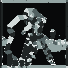
A pixel in texture region can be classified into one of six texture categories based on $E^{\theta}$. Firstly, orientation with biggest energy is texture orientation; but if the energies on all orientations is small enough (smaller than giving threshold $T_{1}$), then there isn’t enough energy of all sub-band, the texture is regarded as smooth; if at least there are two energies are big enough and close to each other, then there isn’t dominant energy, texture is complex. Classifying texture of all pixels, we can obtain a texture matrix. An input image and its classification result are illustrated in Fig.1, in the figuration colors with different grey scales denote different textures.

(a) Input Image

(b) Texture Image

Figure 1: Texture Feature Image

3.3 Parameter selection

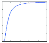
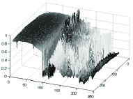
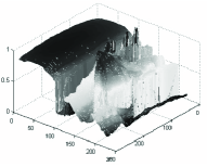
The relationship of $\sigma_{t}$ and the weight function $t\left({\bf\xi,x}\right)$ is showed in Fig.2, where $x$ and $y$ axes represent $\sigma_{t}$ and $t\left({\bf\xi,x}\right)$ respectively. When $\sigma_{t}\rightarrow\infty$, the weight function $t\left({\bf\xi,x}\right)\rightarrow 1$, improved filter approximately equal to standard bilateral filter; if $\sigma_{t}$ is very small, $t\left({\bf\xi,x}\right)$ becomes more important in $\omega\left({\bf x,\xi}\right)$, filtered image relies on texture mainly.

Figure 2: relationship of $t\left({\bf\xi,x}\right)$ and $\sigma_{t}$

4 Simulation results and applications in runway image

4.1 Simulation results

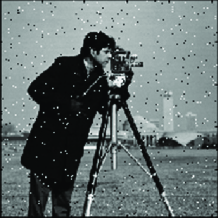
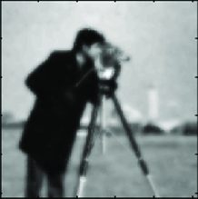
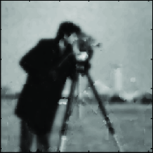
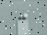
Fig.3 shows the filtering results for a cameraman image added salt and pepper noise after two times filtering. Visualized comparison shows that there is not obviously improvements on edges with different colors. But with similar color, the multilateral filter can keep the image edge detail and have obviously advantage over BF, this result accord with academic analysis. Fig.4 illustrates the amplificatory tower top comparing result. In the input image, the colors of the tower top are closer to the sky. the tower top can not easily be identified in the bilateral filtered image but it is obviously in the multilateral filtered image.

(a) Input Image added noise

(b) bilateral filtering result

(c) Multilateral filtering result

Figure 3: Filtering result comparison of grey scale image

(a) Input Image

(b) bilateral filtering result

(c) Multilateral filtering result

Figure 4: Detail comparison of fig.3

In order to analyze the performance of filters, here we calculate the signal noise ratio (SNR) and the image edge retain exponent $E_{P}$ of the filtered images. The SNR is defined as the ratio of the grey scale value mean square of the input image and the difference of the grey scale value mean square between the input and the filtered image. The image edge retain exponent $E_{P}$ denotes the edge preserving ability of the filters for the image after filtering. The bigger value of $E_{P}$ means the better edge preserving ability. The expression of $E_{P}$ is

$$E_{P}=\frac{\sum_{i=1}^{m}\left|G_{R_{1}}-G_{R_{2}}\right|_{\rm filterred}}{\sum_{i=1}^{m}\left|G_{R_{1}}-G_{R_{2}}\right|_{\rm input}},$$ (8)

here $m$ is the number of samples, $G_{R_{1}}$ and $G_{R_{2}}$ are the grey scale value of neighbor pixels on the image edge of grey scale image respectively.Color image will be converted to grey scale image to calculate $E_{P}$.

Tab.1 shows the statistic dada of the parameter comparison. Here the SNR and the Edge preserving exponent $E_{P}$ are calculated using the whole image. From Tab.1 we can conclude that the SNR and the edge retaining ability of the improved filter exceed the standard bilateral filter, both on horizontal and vertical orientation.

Table 1: Parameter comparison of the bilateral and multilateral filtering results Image added noise

			Edge preserving exponent $E_{P}$
Image added noise	SNR		horizontal		vertical
	Bilateral	multilateral	Bilateral	multilateral	Bilateral	multilateral
Cameraman salt
and pepper’s noise	14.1457	14.3024	0.1259	0.1821	0.3665	0.4464
Cameraman
Gaussian noise	12.7664	12.8754	0.1447	0.2339	0.5459	0.6697
Lena salt
and pepper’s noise	13.4620	13.5794	0.0716	0.1200	0.3290	0.4207
Lena
Gaussian noise	12.0803	12.1530	0.1032	0.1851	0.5410	0.6798
Pears (color image) salt
and pepper’s noise	17.5300	17.6996	0.1131	0.1761	0.3709	0.4514
Pears (color image)
Gaussian noise	16.9481	17.1050	0.1514	0.2266	0.6104	0.7000

In order to compare edge preserve ability of two kinds of filters in different strength of noise, here we give the simulation of Lena added salt and pepper noise. The results of $E_{p\rm Multi}/E_{p\rm Bi}$ are shown in Tab.2, the horizontal and vertical $E_{P}$ comparisons are also included. Here $E_{p\rm Multi}$ and $E_{p\rm Bi}$ represent the edge preserve parameters of multilateral and bilateral filters respectively. From the analysis of Tab.2, the increase of the noise coefficients can cause an obvious increase of the ratio of the edge preserve parameters of the multilateral filter and bilateral filter. Compared with bilateral filter, this indicates that in a more serious noise condition, the multilateral filter has a stronger edge preserving ability.

Table 2: Comparison of edge preserve ability in different noise conditions

Noise coefficient	horizontal	vertical
0.01	1.2992	1.2739
0.03	1.5758	1.2661
0.05	2.0938	1.2753
0.07	2.3385	1.3668

Table 3: Filtering parameter comparison of different $\sigma_{t}$

	Edge preserving exponent $E_{P}$
$\sigma_{t}$	horizontal	vertical	SNR
0.1	0.0340	0.2776	12.9826
1	0.0214	0.2616	12.9527
10	0.0150	0.2339	12.8309
100	0.0150	0.2341	12.8284

Tab.3 gives the comparison of filtering parameter with different $\sigma_{t}$. As $\sigma_{t}$ increase, SNR decrease gradually and the edge preserving parameter has an obvious decrease trend. The simulation results show that as $\sigma_{t}\rightarrow\infty$, SNR and $E_{p}$ tend to the values of bilateral filter. When $\sigma_{t}<0.1$, SNR and $E_{p}$ will go to fixed. This result is consistent with the theoretical analysis.

4.2 Airport runway image filtering

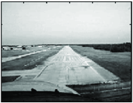
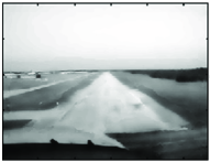
The key of the UAV autonomous landing problem is accurate recognition of the airport runway. However because there are amount of inevitable noise and some disturbs in adopted image sequences, such as the runway marks and the plane shadows, then the accuracy of the runway recognition is effected. So filtering is necessary. When runway and background colors are similar, the effect of standard bilateral filter is not good. In this subsection we / use an improved filtering method to process airport runway image.

(a) Input image and its histogram

(b) Filtered image and its histogram

Figure 5: Airport image filtering

Table 4: Parameter comparison of bilateral and multilateral filters SNR Edge preserving exponent $E_{p}$

		Edge preserving exponent $E_{P}$
SNR		horizontal		vertical
Bilateral	multilateral	Bilateral	multilateral	Bilateral	multilateral
29.4747	29.6184	0.3275	0.3675	0.5219	0.5643

Fig.5 illustrate the filtering results of the airport runway image. From the figure, we can see that the runway information is preserved while the noise is depressed in the filtered image, the mark and shadow on the runway is restrained. It is benefit to segment and recognition. Especially when the grass becomes yellow in autumn and winter or there are highlight disturbs, the colors of runway and background are similar, at this time the standard bilateral filter doesn’t work well, but the multilateral is suitable. Tab.4 gives a quantitatively comparison of the bilateral filtering result and the improved filter result for the input image of fig. 6. We find that the SNR and the edge preserving exponent of the improved filter are better in actual situation .

Here we considered not only the spatial and color closer degree, but also the texture similarity, so the filter performance is improved. The Multilateral filter is simple and non-iterative as the standard bilateral filter, but more robust. The application of the improved filter in airport image processing is effective.

5 Conclusion

By considering the features of the airport runway image filtering, in this paper we proposed an improved bilateral filtering method. Firstly we used the local median energy of steerable filtering decomposition to extract the texture feature of the image, then we gave out the filtered image by using the texture similar, spatial closer and color similar functions. The effect of the weighting function parameters is qualitatively analyzed also. Both the visualized comparisons and the quantitative analysis of the filtering results for the noise added grey scale and the color image showed that the improved method is more effective than the standard bilateral filtering method to preserve the image edge. The advantage of the improved filter is obvious as the noise strength increasing. The filtering results of the airport runway image showed that the improved filtering method can remove noises and disturbs effectively, and has better SNR and edge preserving ability.

While the multilateral filter relies on the texture extraction result. An unappropriate texture feature will yield disturb and influence the filtering result, so before filtering, it is very important to obtain an accurate and appropriate texture feature.

References

- [1] Srikanth Saripalli, James F. Montgomery and Gaurav S.Sukhatme, Vision-based Autonomous Landing of an Unmanned Aerial Vehicle[J]. IEEE. 2002: 2799-2804.
- [2] Srikanth Saripalli, James F. Montgomery, and Gaurav S. Sukhatme. Visually Guided Landing of an Unmanned Aerial Vehicle[J]. IEEE. 2003:371-380.
- [3] J. Hintze. Autonomous Landing of a Rotary Unmanned Aerial Vehicle in a Noncooperative Environment using Machine Vision[D]. Masters Thesis, Brigham Young University, 2004.
- [4] C. Tomasi, R. Manduchi. Bilateral filtering for grey and color image. Proceedings of the 1998 IEEE international conference on computer vision, Bombay, India, 1998.
- [5] D. Barash. A fundamental relationship between bilateral filtering, adaptive smoothing and the non-linear diffusion equation. PAMI, 24(6): 844-847, 2002.
- [6] W. T. Freeman, E. H. Adelson. The design and use of steerable filters. IEEE Trans on Pattern Analysis and Machine Intelligence, 13(9): 891-906, 1991.
- [7] J. Chen, T. N. Pappas, A. Mojsilovic, and B. Rogowwitz, Perceptual color and texture features for segmentation. Human vision and electronic imaging VIII, Jan. 2003, Proc. SPIE Vol. 5007.
- [8] E. P. Simoncelli, WTFreeman, The steerable pyramid: Aflexible architecture for multi-scale derivative computation, Proc, ICIP, vol. III,Oct. 1995, pp. 444-447.