Computing stability of multi-dimensional travelling waves

Abstract

We present a numerical method for computing the pure-point spectrum associated with the linear stability of multi-dimensional travelling fronts to parabolic nonlinear systems. Our method is based on the Evans function shooting approach. Transverse to the direction of propagation we project the spectral equations onto a finite Fourier basis. This generates a large, linear, one-dimensional system of equations for the longitudinal Fourier coefficients. We construct the stable and unstable solution subspaces associated with the longitudinal far-field zero boundary conditions, retaining only the information required for matching, by integrating the Riccati equations associated with the underlying Grassmannian manifolds. The Evans function is then the matching condition measuring the linear dependence of the stable and unstable subspaces and thus determines eigenvalues. As a model application, we study the stability of two-dimensional wrinkled front solutions to a cubic autocatalysis model system. We compare our shooting approach with the continuous orthogonalization method of Humpherys and Zumbrun. We then also compare these with standard projection methods that directly project the spectral problem onto a finite multi-dimensional basis satisfying the boundary conditions.

1 Introduction

Our goal in this paper is to present a practical extension of the Evans function shooting method to computing the stability of multi-dimensional travelling wave solutions to parabolic nonlinear systems. The problem is thus to solve the linear spectral equations for small perturbations of the travelling wave. Hence we need to determine the values of the spectral parameter for which solutions match longitudinal far-field zero boundary conditions and, in more than one spatial dimension, the transverse boundary conditions. These are the eigenvalues. There are two main approaches to solving such eigenvalue problems.

• Projection: Project the spectral equations onto a finite dimensional basis, which by construction satisfies the boundary conditions. Then solve the resulting matrix eigenvalue problem.

• Shooting: Start with a specific value of the spectral parameter and the correct boundary conditions at one end. Shoot/integrate towards the far end. Examine how close this solution is to satisfying the boundary conditions at the far end. Re-adjust the spectral parameter accordingly. Repeat the shooting procedure until the solution matches the far boundary conditions.

The projection method can be applied to travelling waves of any dimension. Its main disadvantage is that to increase accuracy or include adaptation is costly and complicated as we have to re-project onto the finer or adapted basis. Further, from the set of eigenvalues that are produced by the resulting large algebraic eigenvalue problem, care must be taken to distinguish two subsets as follows. In the limit of vanishing discretization scale, one subset corresponds to isolated eigenvalues of finite multiplicity, while the other subset converges to the absolute or essential spectrum, depending on the boundary conditions (see Sandstede and Scheel [26]). The latter subset can be detected by changing the truncated domain size and observing which eigenvalues drift in the complex spectral parameter plane. In contrast, for the shooting method, it is much easier to fine-tune accuracy and adaptivity, and zeros of the matching condition are isolated eigenvalues of finite multiplicity (we do not have to worry about spurious eigenvalues as described above). Its disadvantage though is that by its very description it is a one-dimensional method.

When implementing the shooting method, a Wronskian-like determinant measuring the discrepancy in the boundary matching condition in the spectral problem is typically used to locate eigenvalues in the complex spectral parameter plane. This is known as the Evans function or miss-distance function—see Alexander, Gardner and Jones [1] or Greenberg and Marletta [13]. It is a function of the spectral parameter whose zeros correspond to eigenvalues, i.e. a match. In practice, we match at a point roughly centred at the front. Further for parabolic systems it is typically analytic in the right-half complex parameter plane and the argument principle allows us to globally determine the existence of zeros and therefore unstable eigenvalues by integrating the Evans function along suitably chosen contours.

The one-dimensional label of the Evans function has started to be overturned and in particular Deng and Nii [9], Gesztesy, Latushkin and Makarov [11], and Gesztesy, Latushkin and Zumbrun [12] have extended the Evans function theoretically to multi-dimensions. Importantly from a computational perspective, Humpherys and Zumbrun [19] outlined a computational method crucial to its numerical evaluation in the multi-dimensional scenario. Their method overcame a restriction on the order of the system that could be investigated numerically using shooting, in particular using exterior product spaces. It is based on continuous orhogonalization and is related to integrating along the underlying Grassmannian manifold whilst evolving the coordinate representation for the Grassmannian. More recently Ledoux, Malham and Thümmler [21] provided an alternative (though related) approach to that of Humpherys and Zumbrun. This approach is based on chosen coordinatizations of the Grassmannian manifold and integrating the resulting Riccati systems.

The main idea of this paper is to determine the stability of multi-dimensional travelling waves by essentially combining the two main approaches in the natural way: we project the spectral problem transversely and shoot longitudinally. The basic details are as follows.

1. Transverse to the direction of propagation of the travelling wave we project onto a finite Fourier basis. This generates a large, linear, one-dimensional system of equations for the longitudinal Fourier coefficients.

2. We construct the stable and unstable solution subspaces associated with the longitudinal far-field zero boundary conditions by integrating with given Grassmannian coordinatizations (chosen differently for each subspace).

3. The Evans function is the determinant of the matrix of vectors spanning both subspaces and measures their linear dependence. We evaluate it at an intermediate longitudinal point.

We compare the construction of the stable and unstable solution subspaces by integrating the spectral problem using the continuous orthogonalization method of Humpherys and Zumbrun. We also compare these with standard projection methods that project the spectral problem onto a finite multi-dimensional basis satisfying the boundary conditions and solve the resulting large algebraic eigenvalue problem.

The parabolic nonlinear systems that we will consider here are of the form

$$\partial_{t}U=B\,\Delta U+c\,\partial_{x}U+F(U),$$ (1)

on the cylindrical domain $\mathbb{R}\times\mathbb{T}$. Here $U$ is a vector of component fields and $F(U)$ represents a nonlinear coupling reaction term. The diagonal matrix $B$ encodes the positive constant diffusion coefficients. We suppose we have Dirichlet boundary conditions in the infinite longitudinal direction $x\in\mathbb{R}$ and periodic boundary conditions in the transverse direction $y\in\mathbb{T}$. We assume also, that we are in a reference frame travelling in the longitudinal direction with velocity $c$. Though we assume only two spatial dimensions our subsequent analysis in the rest of this paper is straightforwardly extended to higher dimensional domains which are transversely periodic. We also suppose we have a travelling wave solution $U=U_{c}(x,y)$ of velocity $c$ satisfying the boundary conditions, whose stability is the object of our scrutiny.

As a specific application we consider a cubic autocatalysis reaction-diffusion system that admits wrinkled cellular travelling fronts. They appear as solutions bifurcating from planar travelling wave solutions as the autocatalytic diffusion parameter is increased. The initiation of this first bifurcation is known as the cellular instability and has been studied in some detail in the reaction kinetics and combustion literature; see for example Horváth, Petrov, Scott and Showalter [18] or Terman [29]. However our main interest here is the stability of these cellular fronts themselves. It has been shown by direct numerical simulation of the reaction-diffusion system that the cellular fronts become unstable as the autocatalyst diffusion parameter is increased further—see for example Horváth, Petrov, Scott and Showalter [18] and Malevanets, Careta and Kapral [23]. We apply our multi-dimensional Evans function shooting method to this problem and we reveal the explicit form of the spectrum associated with such fronts. We compare our shooting methods with standard direct projection methods obtaining high accuracy concurrency. We confirm the literature on these instabilities and establish the shooting method as an effective and accurate alternative to standard direct projection methods.

Our paper is structured as follows. In Section 2 we review Grassmannian and Stiefel manifolds. We show how to construct the stable and unstable solution subspaces of the spectral problem using a given Grassmannian coordinatization and define the Evans function using coordinatizations for each subspace. We show how to project the spectral problem onto a finite dimensional transverse basis in detail in Section 3. A large portion of numerical effort is devoted to accurately constructing the multi-dimensional fronts whose stability we wish to study, and in Section 4 we detail the technique we used to do this. In Section 5 we outline our main application—the cubic autocatalysis problem—and review the known travelling wave solutions and stability properties. We then bring to bear our full range of numerical techniques to the cubic autocatalysis problem in Section 6, comparing their accuracy. In Section 7 we provide some concluding remarks and outline future directions of investigation.

2 Review: Grassmann flows and spectral matching

2.1 Grassmannian coordinate representations

A $m$-frame is a $m$-tuple of $m\leq n$ linearly independent vectors in ${\mathbb{C}}^{n}$. The Stiefel manifold ${\mathbb{V}}(n,m)$ of $m$-frames is the open subset of ${\mathbb{C}}^{n\times m}$ of all $m$-frames centred at the origin. Hence any element $Y\in{\mathbb{V}}(n,m)$ can be represented by an $n\times m$ matrix of rank $m$:

$$Y=\begin{pmatrix}Y_{11}&\cdots&Y_{1m}\\ \vdots&&\vdots\\ Y_{n1}&\cdots&Y_{nm}\end{pmatrix}.$$ (2)

The set of $m$ dimensional subspaces of ${\mathbb{C}}^{n}$ forms a complex manifold $\mathrm{Gr}(n,m)$ called the Grassmann manifold of $m$-planes in ${\mathbb{C}}^{n}$; it is compact and connected (see Steenrod [28, p. 35] or Griffiths and Harris [14, p. 193]). There is a quotient map from ${\mathbb{V}}(n,m)$ to ${\mathrm{Gr}}(n,m)$, sending each $m$-frame centred at the origin to the $m$-plane it spans—see Milnor-Stasheff [24, p. 56]. Any $m$-plane in ${\mathbb{C}}^{n}$ can be represented by an $n\times m$ matrix of rank $m$, like $Y$ above. However any two such matrices $Y$ and $Y^{\prime}$ related by a rank $m$ transformation $u\in{\mathrm{GL}}(k)$, so that $Y^{\prime}=Yu$, will represent the same $m$-plane. Hence we can cover the Grassmann manifold ${\mathrm{Gr}}(n,m)$ by coordinate patches ${\mathbb{U}}_{\mathfrak{i}}$, labelled with multi-index ${\mathfrak{i}}=\{i_{1},\ldots,i_{m}\}\subset\{1,\ldots,n\}$, where ${\mathbb{U}}_{\mathfrak{i}}$ is the set of $m$-planes $Y\in{\mathrm{Gr}}(n,m)$, which have a matrix representation $y_{{\mathfrak{i}}^{\circ}}\in{\mathbb{C}}^{n\times m}$ whose $m\times m$ submatrix, designated by the rows ${\mathfrak{i}}$, is the identity matrix. Each such patch is an open dense subset of ${\mathrm{Gr}}(n,m)$ isomorphic to ${\mathbb{C}}^{(n-m)m}$. For example, if ${\mathfrak{i}}=\{1,\ldots,m\}$, then ${\mathbb{U}}_{\{1,\ldots,m\}}$ can be uniquely represented by a matrix of the form

$$y_{{\mathfrak{i}}^{\circ}}=\begin{pmatrix}{I}_{m}\\ \hat{y}\end{pmatrix}$$ (3)

with ${\mathfrak{i}}^{\circ}=\{m+1,\ldots,n\}$ and $\hat{y}\in{\mathbb{C}}^{(n-m)m}$. For each ${\mathfrak{i}}$, there is a bijective map $\varphi_{{\mathfrak{i}}}\colon{\mathbb{U}}_{\mathfrak{i}}{\rightarrow}{\mathbb{C}}^{(n-m)m}$ given by $\varphi_{{\mathfrak{i}}}\colon y_{{\mathfrak{i}}^{\circ}}\mapsto\hat{y}$, representing the local coordinate chart for the coordinate patch ${\mathbb{U}}_{\mathfrak{i}}$. For more details see Griffiths and Harris [14, p.193–4].

2.2 Riccati flow

Consider a non-autonomous linear vector field defined on the Stiefel manifold of the form $V(x,Y)=A(x)\,Y$, where $Y\in{\mathbb{V}}(n,m)$ and $A\colon\mathbb{R}{\rightarrow}\mathfrak{gl}(n)$, the general linear algebra of rank $n$ matrices. Following the exposition in Ledoux, Malham and Thümmler [21], fix a coordinate patch ${\mathbb{U}}_{\mathfrak{i}}$ for ${\mathrm{Gr}}(n,m)$ for some ${\mathfrak{i}}$, and decompose $Y\in{\mathbb{V}}(n,m)$ into

$$Y=y_{{\mathfrak{i}}^{\circ}}u.$$

If we substitute this form into the ordinary differential system $Y^{\prime}=V(x,Y)$ we obtain:

$$y_{{\mathfrak{i}}^{\circ}}^{\prime}u+y_{{\mathfrak{i}}^{\circ}}u^{\prime}=(A_{\mathfrak{i}}+A_{{\mathfrak{i}}^{\circ}}y_{{\mathfrak{i}}^{\circ}})\,u,$$

where $A_{\mathfrak{i}}$ denotes the submatrix obtained by restricting the matrix $A(x)$ to its ${\mathfrak{i}}$th columns. If we project this last system onto its ${\mathfrak{i}}^{\circ}$th and ${\mathfrak{i}}$th rows, respectively, we generate the following pair of equations for the coordinate chart variables $\hat{y}=\varphi_{\mathfrak{i}}\circ y_{{\mathfrak{i}}^{\circ}}$ and transformations $u$, respectively:

$$\hat{y}^{\prime} =c+d\hat{y}-\hat{y}a-\hat{y}b\hat{y}$$ (4a)

and

$$u^{\prime} =(a+b\hat{y})\,u.$$ (4b)

Here $a$, $b$, $c$ and $d$ denote the ${\mathfrak{i}}\times{\mathfrak{i}}$, ${\mathfrak{i}}\times{\mathfrak{i}}^{\circ}$, ${\mathfrak{i}}^{\circ}\times{\mathfrak{i}}$ and ${\mathfrak{i}}^{\circ}\times{\mathfrak{i}}^{\circ}$ submatrices of $A$, respectively.

We observe that the flow on the Stiefel manifold ${\mathbb{V}}(n,m)$ generated by the linear vector field $V(x,Y)$ can be decomposed into an independent Riccati flow in the coordinate chart variables of a fixed coordinate patch ${\mathbb{U}}_{\mathfrak{i}}$ of ${\mathrm{Gr}}(n,m)$, and a slaved linear flow of transformations in ${\mathrm{GL}}(m)$. Hence we can reconstruct the flow on the Stiefel manifold generated by the linear vector field $V(x,Y)$, by simply solving the Riccati equation above, and then if required, subsequently integrating the linear equation for the transformations. In general, solutions to the Riccati equation (4a) can blow up. However, this is simply the manifestation of a poorly chosen local representative coordinate patch. This can be gleaned from the fact that simultaneously the determinant of $u$ becomes zero—afterall the linear Stiefel flow, with globally smooth coefficients, does not blow up. To resolve this, we simply change patch and keep a record of the determinant of the patch swapping transformation. Further details and strategies can be found in Ledoux, Malham and Thümmler [21].

2.3 Drury–Oja flow

The continuous orthogonalization method of Humpherys and Zumbrun [19] can be thought of as the flow on the Grassmann manifold corresponding to the linear vector field $V$, with the coordinatization evolving according to a given unitary flow (see Ledoux, Malham and Thümmler [21]). Indeed their method is specified by a Drury–Oja flow for the $n\times m$ orthogonal matrix $Q$, together with the flow for the determinant of the matrix $R$, in the $QR$-decomposition of $Y$:

$$Q^{\prime} =({I}_{n}-QQ^{\dagger})A(x)Q,$$ (5a)

$$(\det R)^{\prime} =\mathrm{Tr}\bigl{(}Q^{\dagger}A(x)Q\bigr{)}(\det R).$$ (5b)

Here $Q^{\dagger}$ denotes the Hermitian transpose of $Q$. In practice the determinant of $R$ is exponentially rescaled—see Humpherys and Zumbrun [19]. We also did not find it necessary to apply any of the stabilization techniques suggested therein.

2.4 Spectral problem

Consider the linear spectral problem on ${\mathbb{R}}$ with spectral parameter $\lambda$ in standard first order form with coefficient matrix $A(x;\lambda)\in{\mathbb{C}}^{n\times n}$:

$$Y^{\prime}=A(x;\lambda)\,Y.$$ (6)

We assume there exists a subdomain $\Omega\subset{\mathbb{C}}$ containing the right-half complex plane, that does not intersect the essential spectrum. For $\lambda\in\Omega$, we know that there exists exponential dichotomies on $\mathbb{R}^{-}$ and $\mathbb{R}^{+}$ with the same Morse index $m$ in each case (see Sandstede [25]). Hence for $\lambda\in\Omega$, let $Y^{-}(x;\lambda)\in{\mathbb{V}}(n,m)$ denote the matrix whose columns are solutions to (6) which span the unstable subspace of solutions decaying exponentially to zero as $x{\rightarrow}-\infty$, and let $Y^{+}(x;\lambda)\in{\mathbb{V}}(n,n-m)$ denote the matrix whose columns are the solutions which span the stable subspace of solutions decaying exponentially to zero as $x{\rightarrow}+\infty$. The values of spectral parameter $\lambda$ for which the columns of $Y^{-}$ and columns of $Y^{+}$ are linearly dependent on ${\mathbb{R}}$ are pure-point eigenvalues.

2.5 Evans determinant

The Evans function $D(\lambda)$ is the measure of the linear dependence between the two basis sets $Y^{-}$ and $Y^{+}$:

$$D(\lambda)\equiv\mathrm{e}^{-\int_{0}^{x}\mathrm{Tr}A(\xi;\lambda)\,\mathrm{d}\xi}\,\mathrm{det}\bigl{(}Y^{-}(x;\lambda)\,\,Y^{+}(x;\lambda)\bigr{)},$$ (7)

(see Alexander, Gardner and Jones [1] or Sandstede [25] for more details). Note that for the decompositions $Y^{-}=y_{{\mathfrak{i}}_{-}^{\circ}}u_{-}$ and $Y^{+}=y_{{\mathfrak{i}}_{+}^{\circ}}u_{+}$, assuming $\det\,u_{-}\neq 0$ and $\det\,u_{+}\neq 0$, we have

$$\det\bigl{(}Y^{-}\,Y^{+}\bigr{)}=\det\begin{pmatrix}y_{{\mathfrak{i}}_{-}^{\circ}}&y_{{\mathfrak{i}}_{+}^{\circ}}\end{pmatrix}\cdot\det\,u_{-}\cdot\det\,u_{+}.$$

Let $Y_{0}^{-}(\lambda)$ denote the $n\times m$ matrix whose columns are the $m$ eigenvectors of $A(-\infty;\lambda)$ corresponding to eigenvalues with a positive real part. Analogously let $Y_{0}^{+}(\lambda)$ denote the $n\times(n-m)$ matrix whose columns are the $(n-m)$ eigenvectors of $A(+\infty;\lambda)$ corresponding to eigenvalues with a negative real part.

Suppose we fix a coordinate patch for ${\mathrm{Gr}}(n,m)$ labelled by ${\mathfrak{i}}_{-}$ (which has cardinality $m$). We integrate the corresponding Riccati differential problem (4a) for $\hat{y}_{-}=\varphi_{{\mathfrak{i}}_{-}}\circ y_{{\mathfrak{i}}_{-}^{\circ}}$ from $x=-\infty$ to $x=x_{\ast}$. The initial data $\hat{y}_{-}(-\infty;\lambda)$ is generated by postmultiplying the ${\mathfrak{i}}_{-}^{\circ}\times\{1,\ldots,m\}$ submatrix of $Y_{0}^{-}(\lambda)$ by the inverse of the ${\mathfrak{i}}_{-}\times\{1,\ldots,m\}$ submatrix of $Y_{0}^{-}(\lambda)$ (i.e. perform the simple decomposition into $y_{{\mathfrak{i}}_{-}^{\circ}}$ and $u_{-}$ for $Y_{0}^{-}(\lambda)$, and use the ${\mathfrak{i}}_{-}^{\circ}\times\{1,\ldots,m\}$ block of $y_{{\mathfrak{i}}_{-}^{\circ}}$ as the initial data for $\hat{y}_{-}$). Similarly we fix a patch for ${\mathrm{Gr}}(n,n-m)$ labelled by ${\mathfrak{i}}_{+}$ (with cardinality $(n-m)$) and integrate the Riccati differential problem (4a) for $\hat{y}_{+}=\varphi_{{\mathfrak{i}}_{+}}\circ y_{{\mathfrak{i}}_{+}^{\circ}}$ from $x=+\infty$ to $x=x_{\ast}$. We perform the analogous decomposition on $Y^{+}_{0}(\lambda)$ with index ${\mathfrak{i}}_{+}$ to generate the initial data $\hat{y}_{+}(+\infty;\lambda)$. If the solutions to both Riccati problems do not blow up, so that $\det u_{-}(x;\lambda)\neq 0$ for all $x\in(-\infty,x_{\ast}]$ and $\det u_{+}(x;\lambda)\neq 0$ for all $x\in[x_{\ast},\infty)$, then we define the modified Evans function, which is analytic in $\lambda$, by

$$D(\lambda;x_{\ast})\equiv\det\begin{pmatrix}y_{{\mathfrak{i}}_{-}^{\circ}}(x_{\ast};\lambda)&y_{{\mathfrak{i}}_{+}^{\circ}}(x_{\ast};\lambda)\end{pmatrix},$$ (8)

where $x_{\ast}\in{\mathbb{R}}$ is the matching point. In our practical implementation in Section 5, we took the patches labelled by ${\mathfrak{i}}_{-}=\{1,\ldots,m\}$ and ${\mathfrak{i}}_{+}=\{m+1,\ldots,n\}$ for the left and right problems, respectively. We used the generally accepted rule of thumb for Evans function calculations: to match at a point roughly centred at the front. In our example application we took $x_{*}=50$, and did not observe singularities in $\hat{y}^{-}$ or $\hat{y}^{+}$. However generally, varying $x_{\ast}$ may introduce singularities for $\hat{y}^{-}$ or $\hat{y}^{+}$ in their respective domains $(-\infty,x_{\ast}]$ and $[x_{\ast},\infty)$. Indeed this was observed in several examples considered in Ledoux, Malham and Thümmler [21]. There, a robust remedy is provided, which on numerical evidence, allows matching anywhere in the computational domain (and which in future work we intend to apply to our context here).

If we use the Humpherys and Zumbrun continuous orthogonalization approach then we define the Evans function to be

$$D_{\text{HZ}}(\lambda;x_{\ast})\equiv\det\bigl{(}Q^{-}(x_{\ast};\lambda)~{}Q^{+}(x_{\ast};\lambda)\bigr{)}\cdot\det R^{-}(x_{\ast};\lambda)\cdot\det R^{+}(x_{\ast};\lambda).$$ (9)

This is analytic in $\lambda$ when we include the $\det R^{\pm}$ terms.

2.6 Angle between subspaces

We can also measure the angle between the unstable and stable linear subspaces ${\mathbb{V}}(n,m)$ and ${\mathbb{V}}(n,n-m)$, see Björck and Golub [7]. When the columns of the matrices $Y^{-}(x;\lambda)$ and $Y^{+}(x;\lambda)$ which span ${\mathbb{V}}(n,m)$ and ${\mathbb{V}}(n,n-m)$, respectively, are nearly linearly dependent the angle will be small. It is defined as follows—without loss of generality we assume $m\geq n/2$. Let $Q^{-}$ and $Q^{+}$ be unitary bases for ${\mathbb{V}}(n,m)$ and ${\mathbb{V}}(n,n-m)$. They are specified by the $QR$-decompositions $Y^{-}=Q^{-}R^{-}$ and $Y^{+}=Q^{+}R^{+}$. The cosine of the smallest angle $\theta$ between ${\mathbb{V}}(n,m)$ and ${\mathbb{V}}(n,n-m)$ is given by the largest singular value of the matrix $(Q^{-})^{\dagger}Q^{+}$. However when $\theta$ is small it is more accurate to compute $\sin\theta$, which is given by the smallest singular value of

$$\big{(}{I}_{n}-Q^{-}(Q^{-})^{\dagger}\bigr{)}Q^{+}.$$

Hence if the singular values of this matrix are $\sigma_{i}$, $i=1,\ldots,n-m$, define

$$\theta(\lambda;x_{\ast})\equiv\arcsin\min_{i=1,\ldots,n-k}\sigma_{i},$$

where again, $x_{\ast}$ is the matching point. Eigenvalues correspond to zeros of $\theta(\lambda;x_{\ast})$.

3 Projection onto a finite transverse Fourier basis

Consider the parabolic nonlinear system (1) posed on the cylindrical domain $\mathbb{R}\times\mathbb{T}$. Recall that we assume Dirichlet boundary conditions in the infinite longitudinal direction $x\in\mathbb{R}$ and periodic boundary conditions in the transverse direction $y\in\mathbb{T}$ (here $\mathbb{T}$ is the one-torus with period/circumference $L$). Suppose we have a travelling wave solution $U=U_{c}(x,y)$ of velocity $c$ satisfying the boundary conditions. The stability of this solution is determined by the spectrum of the linear differential operator

$$\mathcal{L}=B\Delta+c\,\partial_{x}+\mathrm{D}F(U_{c}),$$ (10)

where $\mathrm{D}F$ is the Jacobian of the interaction term. Hence the eigenvalue problem is

$$B\Delta U+c\,\partial_{x}U+\mathrm{D}F(U_{c})U=\lambda U.$$ (11)

We wish to define and compute the Evans function for this spectral problem. The idea is to perform a Fourier decomposition in the transverse direction. This transforms the problem to a one-dimensional problem, for which we can apply the Evans function shooting approach. Hence suppose that we can write

$$U(x,y)=\sum_{k=-\infty}^{\infty}{\hat{U}}_{k}(x)\,\mathrm{e}^{iky/{\tilde{L}}},$$ (12)

where ${\hat{U}}_{k}\in\mathbb{C}^{N}$ are the Fourier coefficients (with $N$ denoting the number of components of $U$) and ${\tilde{L}}=2\pi L$—this implicitly restricts our attention to perturbations $U$ with period $L$. Similarly, we expand $\mathrm{D}F(U_{c})$ as

$$\mathrm{D}F(U_{c}(x,y))=\sum_{k=-\infty}^{\infty}{\hat{D}}_{k}(x)\,\mathrm{e}^{iky/{\tilde{L}}},$$ (13)

where the Fourier coefficients ${\hat{D}}_{k}\in\mathbb{C}^{N\times N}$. Substituting our Fourier expansions for $U$ and $\mathrm{D}F(U_{c})$ in (12) and (13) in the eigenvalue problem (11) yields

$$B\,(\partial_{xx}+\partial_{yy})\sum_{k=-\infty}^{\infty}{\hat{U}}_{k}\,\mathrm{e}^{iky/{\tilde{L}}}+c\,\partial_{x}\sum_{k=-\infty}^{\infty}{\hat{U}}_{k}\,\mathrm{e}^{iky/{\tilde{L}}}\\ +\sum_{\ell=-\infty}^{\infty}{\hat{D}}_{\ell}\,\mathrm{e}^{i\ell y/{\tilde{L}}}\sum_{k=-\infty}^{\infty}{\hat{U}}_{k}\,\mathrm{e}^{iky/{\tilde{L}}}=\lambda\sum_{k=-\infty}^{\infty}{\hat{U}}_{k}\,\mathrm{e}^{iky/{\tilde{L}}}.$$

Reordering the double sum

$$\sum_{\ell=-\infty}^{\infty}{\hat{D}}_{\ell}\,\mathrm{e}^{i\ell y/{\tilde{L}}}\sum_{k=-\infty}^{\infty}{\hat{U}}_{k}\,\mathrm{e}^{iky/{\tilde{L}}}=\sum_{k=-\infty}^{\infty}\sum_{\nu=-\infty}^{\infty}{\hat{D}}_{k-\nu}{\hat{U}}_{\nu}\,\mathrm{e}^{iky/{\tilde{L}}},$$

yields that for all $k\in{\mathbb{Z}}$, we must have

$$\partial_{xx}{\hat{U}}_{k}-(k/{\tilde{L}})^{2}{\hat{U}}_{k}+c\,B^{-1}\partial_{x}{\hat{U}}_{k}+\sum_{\nu=-\infty}^{\infty}B^{-1}{\hat{D}}_{k-\nu}{\hat{U}}_{\nu}=\lambda B^{-1}{\hat{U}}_{k}.$$

In practical implementation, we consider only the first $K$ Fourier modes. Hence we replace the above infinite system of equations by following finite system of equations which we now also express in first order form:

$$\partial_{x}{\hat{U}}_{k} ={\hat{P}}_{k},$$ (14a)

$$\partial_{x}{\hat{P}}_{k} =\lambda B^{-1}{\hat{U}}_{k}+(k/{\tilde{L}})^{2}{\hat{U}}_{k}-c\,B^{-1}{\hat{P}}_{k}-\sum_{\nu=-K}^{K}B^{-1}{\hat{D}}_{k-\nu}{\hat{U}}_{\nu},$$ (14b)

for $k=-K,-K+1,\ldots,K$. This is a large system of ordinary differential equations involving the spectral parameter $\lambda$, so we can apply the standard Evans function approach to it. In matrix form this is

$$\partial_{x}\begin{pmatrix}{\hat{U}}\\ {\hat{P}}\end{pmatrix}=\begin{pmatrix}O_{N(2K+1)}&I_{N(2K+1)}\\ A_{3}(x;\lambda)&A_{4}\end{pmatrix}\begin{pmatrix}{\hat{U}}\\ {\hat{P}}\end{pmatrix},$$ (15)

where ${\hat{U}}$ is the vector of $\mathbb{C}^{N}$-valued components ${\hat{U}}_{-K}$, ${\hat{U}}_{-K+1}$, …, ${\hat{U}}_{K}$ and ${\hat{P}}$ is the vector of $\mathbb{C}^{N}$-valued components ${\hat{P}}_{-K}$, ${\hat{P}}_{-K+1}$, …, ${\hat{P}}_{K}$. The lower right block matrix is $A_{4}=-c\,B^{-1}\otimes I_{2K+1}$. The lower left block matrix is given by $A_{3}=\tilde{A}_{3}(\lambda)+\hat{A}_{3}(x)$ where if we set $E_{k}(\lambda)\equiv\lambda B^{-1}+(k/{\tilde{L}})^{2}I_{N}$ then

$$\tilde{A}_{3}(\lambda)=\begin{pmatrix}E_{-K}(\lambda)&O&\cdots&O\\ O&E_{-K+1}(\lambda)&\cdots&O\\ \vdots&\vdots&\ddots&\vdots\\ O&\cdots&O&E_{+K}(\lambda)\end{pmatrix}$$

and

$$\hat{A}_{3}(x)=-B^{-1}\otimes\begin{pmatrix}{\hat{D}}_{0}&{\hat{D}}_{-1}&\cdots&{\hat{D}}_{-2K}\\ {\hat{D}}_{1}&{\hat{D}}_{0}&\cdots&{\hat{D}}_{-2K+1}\\ \vdots&\vdots&\ddots&\vdots\\ {\hat{D}}_{2K}&{\hat{D}}_{2K-1}&\cdots&{\hat{D}}_{0}\end{pmatrix}.$$

A similar Galerkin approximation for nonplanar fronts can be found in Gesztesy, Latushkin and Zumbrun [12, p. 28,37].

4 The freezing method

To study the long-time behaviour of the wrinkled front solution we use the method of freezing travelling waves described in Beyn and Thümmler [6] and analyzed in Thümmler [30]. This method transports the problem into a moving frame whose velocity is computed during the computation. For the travelling waves whose stability is our concern here, the freezing method has two advantages over direct simulation: Firstly, we can do long-time computations of time dependent (for example oscillating) solutions. This is because the method picks out the correct speed for the moving frame in which the wave is roughly stationary (in particular it does not drift out of the chosen domain). Secondly, the freezing method can be used to obtain a suitably accurate guess for the waveform, which can then be used to initiate a Newton solver that computes the travelling wave as a stationary solution in the co-moving frame. For completeness we will briefly review the idea of the freezing method here. Consider a parabolic nonlinear system of form (1) in a stationary frame of reference:

$$\partial_{t}U=B\,\Delta U+F(U).$$ (16)

If we substitute the ansatz $U(x,y,t)=V(x-\gamma(t),y,t)$ into this equation, where $\gamma(t)$ is the unknown reference position for a wave travelling in the longitudinal $x$-direction, we generate the partial differential equation for $V$ and $\gamma^{\prime}$:

$$\partial_{t}V=B\,\Delta V+\gamma^{\prime}(t)\partial_{x}V+F(V).$$ (17a)

In order to compensate for the additional degree of freedom which has been introduced by the unknown position $$\gamma$$, we specify the following additional algebraic constraint

$$0=\int_{{\mathbb{R}}\times\mathbb{T}}\bigl{(}\partial_{x}\hat{V}(x,y,t)\bigr{)}^{\mathrm{T}}\bigl{(}\hat{V}(x,y,t)-V(x,y,t)\bigr{)}\,\mathrm{d}x\,\mathrm{d}y.$$ (17b)

This constraint selects a unique solution from the one-parameter group of possible solutions generated by longitudinal translation. It is a phase condition that normalizes the system with respect to a given template function—for example a suitable choice is to set $\hat{V}(x,y,t)$ to be the initial data $V(x,y,0)$. Hence we have generated a partial differential algebraic system (17), for the unknowns $V(x,y,t)$ and $\zeta(t)=\gamma^{\prime}(t)$, with initial data $V(x,y,0)$ and $\zeta(0)$ within the attractive set of the stable travelling wave and its velocity.

A stationary solution $(V,\zeta)=(V_{c},c)$ of the partial differential algebraic system (17) represents a travelling wave solution $U_{c}(x,y,t)=V_{c}(x-ct,y)$ with fixed speed $c$ to the parabolic nonlinear problem (16). If the travelling wave $U_{c}$ is stable then the stationary solution $(V_{c},c)$ is also stable and the time evolution of partial differential algebraic system (17) will converge to $(V_{c},c)$. Thus the numerical method consists of solving the partial differential algebraic system (17) until the solution $(V,\zeta)$ has reached the equilibrium $(V_{c},c)$. Alternatively one can also solve the partial differential algebraic system (17) until some time $t=T$ when the solution is deemed sufficiently close to equilibrium and then use a direct method (e.g. Newton’s method) to solve the stationary equation

$$0 =B\,\Delta v+\theta\partial_{x}v+F(v),$$ (18a)

$$0 =\int_{{\mathbb{R}}\times\mathbb{T}}\bigl{(}\partial_{x}\hat{V}(x,y)\bigr{)}^{\mathrm{T}}\bigl{(}\hat{V}(x,y)-v(x,y)\bigr{)}\,\mathrm{d}x\,\mathrm{d}y,$$ (18b)

for $(v,\theta)$ starting with initial values $v_{0}(x,y)=V(x,y,T)$ and $\theta_{0}=\zeta(T)$.

5 Review: autocatalytic system

As our model application we consider the cubic autocatalysis system

$$u_{t} =\Delta u+c\partial_{x}u-uv^{2},$$ (19a)

$$v_{t} =\delta\Delta v+c\partial_{x}v+uv^{2}.$$ (19b)

Here $u(x,y,t)$ is the concentration of the reactant and $v(x,y,t)$ is the concentration of the autocatalyst, in the infinitely extended medium $(x,y)\in\mathbb{R}\times\mathbb{T}$. In the far field, we suppose $(u,v)$ approaches the stable homogenenous steady state $(0,1)$ as $x\rightarrow-\infty$, and the unstable homogeneous steady state $(1,0)$ as $x\rightarrow+\infty$. The parameter $\delta$ is the ratio of the diffusivity of the autocatalyst to that of the reactant. This system is is globally well-posed for smooth initial data, and any finite $\delta>0$.

From Billingham and Needham [4] we know that, in one spatial dimension, a unique heteroclinic connection between the unstable and stable homogeneous steady states exists for wavespeeds $c\geq c_{\min}$. The unique travelling wave for $c=c_{\min}$ converges exponentially to the homogeneous steady states. They are readily constructed by shooting (see for example Balmforth, Craster and Malham [3]) and represent the planar front solution referred to hereafter.

It is well known that these planar travelling wave solutions become unstable to transverse perturbations when $\delta$ is greater than a critical ratio $\delta_{\mathrm{cr}}\approx 2.3$ (from Malevanets, Careta and Kapral [23, p. 4733]), and our transverse domain is sufficiently large. This is known as the cellular instability—see for example Terman [29], Horváth, Petrov, Scott and Showalter [18] and Malevanets, Careta and Kapral [23]. Calculating the spectrum that reveals the mechanism of the instability is also straightforward. If we consider small perturbations about the underlying planar travelling wave solution of the form $\hat{U}(x)\mathrm{e}^{\lambda t+\mathrm{i}(k/\tilde{L})y}$, for any $k\in\mathbb{Z}$, then the associated linear operator ${\mathcal{L}}$ whose spectrum we wish to determine has the form

$${\mathcal{L}}=B\bigl{(}\partial_{xx}-(k/\tilde{L})^{2}I\bigr{)}+c\,\partial_{x}+\mathrm{D}F(U_{c}).$$ (20)

The spectrum of ${\mathcal{L}}$ consists of the pure-point spectrum, i.e. isolated eigenvalues of finite multiplicity, together with the essential spectrum. By a result of Henry [15], if we consider ${\mathcal{L}}$ as an operator on the space of square integrable functions, we know that the essential spectrum is contained within the parabolic curves of the continuous spectrum in left-half complex plane. The continuous spectrum for this model problem is given for all $\mu\in\mathbb{R}$ and each fixed $k\in\mathbb{Z}$, by the locus in the complex $\lambda$-plane of the curves

$$\lambda =-\delta(k/\tilde{L})^{2}+\mathrm{i}c\mu-\delta\mu^{2},$$

$$\lambda =-1-\delta(k/\tilde{L})^{2}+\mathrm{i}c\mu-\delta\mu^{2},$$

$$\lambda =-(k/\tilde{L})^{2}+\mathrm{i}c\mu-\mu^{2},$$

where the last curve appears with multiplicity two. Hence the continuous spectrum touches the imaginary axis at the origin when $k$ is zero. The origin is a simple eigenvalue for ${\mathcal{L}}$ due to translational invariance of the underlying travelling wave $U_{c}(x)$ in the longitudinal direction. Thus, even though the essential spectrum does not affect linear stability, we cannot automatically deduce asymptotic stability unless we consider a gently weighted space of square integrable functions, which will shift the essential spectrum to the left.

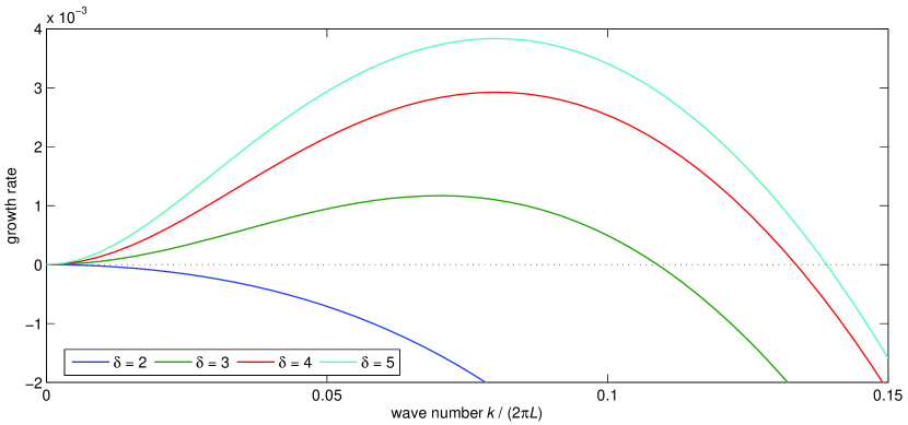
We now notice that the spectral problem for the linear differential operator ${\mathcal{L}}$ is fourth order and one-dimensional, the transverse perturbation information is encoded though the transverse wavenumber parameter $k$. Hence we can employ the Evans function shooting approach, in particular in Figure 1 we plot the dispersion relation for planar fronts corresponding to different values of the physical parameter $\delta$. The dispersion relation gives the relationship between the real part of the exponential growth factor of small perturbations, $\mathrm{Re}(\lambda)$, and transverse wave number $k$ (in fact to make comparisons later easier we have used $k/\tilde{L}$ on the abscissa). To construct the graph shown, we locate zeros of the Evans function on the real $\lambda$ axis and follow them as the transverse wave number $k$ is varied. We see in Figure 1 that the interval $(0,k_{\delta})$ of unstable transverse wavenumbers $k$ increases as $\delta$ increases (at least up to $\delta=5$). The wavenumber where the maximum of $\mathrm{Re}(\lambda)$ occurs has largest growth and is thus typically the transverse mode expressed in the dynamics.

Fig. 1: Dispersion relations for the planar front for different values of $\delta$. For $\delta=2$, all perturbations decay and the planar front is linearly stable, but for the other values of $\delta$ there is a growing interval $(0,k_{\delta})$ of unstable transverse wavenumbers.

However our real concern here is the stability of the wrinkled cellular fronts themselves as we increase the diffusion ratio parameter $\delta$ beyond $\delta_{\mathrm{cr}}$. We know the planar waves are unstable in this regime and the question is whether the bifurcating wrinkled cellular fronts are stable for values of $\delta$ just beyond $\delta_{\mathrm{cr}}$ but do become unstable at another critical value of $\delta$. Using direct simulations of the reaction-diffusion system Malevanets, Careta and Kapral [23] demonstrated that when $\delta=5$ the transverse structure of the propagating fronts was very complex with spatio-temporal dynamics of its own. Our goal is to elicit in practice the initial mechanisms that precipitate the behaviour they observe through a careful study of the spectra of the underlying multi-dimensional travelling fronts.

6 Numerics

6.1 The method

We will compute the spectrum of the two-dimensional travelling front by computing the Evans function associated with the linear operator $\mathcal{L}$ defined in (10). First, we compute the front with the freezing method as explained in Section 4. Then as in Section 3, we project the problem onto a finite number of transverse Fourier modes $k=-K,\ldots,K$. This generates the large linear system (15) which is of the standard linear form (6) where the coefficient matrix is given by

$$A(x;\lambda)=\begin{pmatrix}O_{N(2K+1)}&I_{N(2K+1)}\\ A_{3}(x;\lambda)&A_{4}\end{pmatrix},$$

where the matrices $A_{3}$ and $A_{4}$ are explicitly given at the end of Section 3. This coefficient matrix depends on both the travelling wave solution $U_{c}$ and the spectral parameter $\lambda$. It also depends on the nonlinear reaction term. For our autocatalytic problem the Jacobian $\mathrm{D}F$ of the nonlinear reaction term and its Fourier transform ${\hat{D}}$ are given by

$$\mathrm{D}F(U)=\begin{pmatrix}-v^{2}&-2uv\\ v^{2}&2uv\end{pmatrix}\qquad\text{and}\qquad{\hat{D}}=\begin{pmatrix}-{\hat{v}}*{\hat{v}}&-2{\hat{u}}*{\hat{v}}\\ {\hat{v}}*{\hat{v}}&2{\hat{u}}*{\hat{v}}\end{pmatrix},$$

where ${\hat{u}}$ and ${\hat{v}}$ are the Fourier transforms of $u$ and $v$ respectively, and $*$ denotes the convolution defined by $({\hat{u}}*{\hat{v}})_{k}=\sum_{\ell=-\infty}^{\infty}{\hat{u}}_{\ell}{\hat{v}}_{k-\ell}$.

As described in Section 2.5, we construct the unstable subspace $Y_{0}^{-}(\lambda)$ of (15) at $x=-\infty$, as the matrix whose columns are the eigenvectors of $A(-\infty;\lambda)$ corresponding to eigenvalues with a positive real part. Similarly we construct the stable subspace $Y_{0}^{+}(\lambda)$ at $x=+\infty$ from the eigenvectors of $A(+\infty;\lambda)$ corresponding to eigenvalues with a negative real part. Then to construct the modified Evans function (8) at the matching point $x_{*}$ we proceeded as follows (for both the planar and wrinkled front cases for the autocatalytic problem below). The full system is of size $n=4(2K+1)$. We use the coordinate patch identified by ${\mathfrak{i}}_{-}=\{1,\ldots,m\}$ where $m=2(2K+1)$ for the interval $(-\infty,x_{*}]$. On this interval we solve the Riccati equation (4a) for $\hat{y}_{-}$; with the chosen coordinate patch, the coefficient matrices in the Riccati equation are $a=O_{m}$, $b=I_{m}$, $c=A_{3}$ and $d=A_{4}$. The initial data for $\hat{y}_{-}$ is simply the lower $(n-m)\times m$ block of $Y_{0}^{-}(\lambda)$ postmultiplied by the inverse of the upper $m\times m$ block of $Y_{0}^{-}(\lambda)$. For the interval $[x_{*},+\infty)$ we use the coordinate patch identified by ${\mathfrak{i}}_{+}=\{m+1,\ldots,n\}$. We solve the Riccati equation (4a) for $\hat{y}_{+}$; the coefficient matrices in this case are $a=A_{4}$, $b=A_{3}$, $c=I_{m}$ and $d=O_{m}$. The initial data for $\hat{y}_{+}$ is the upper $m\times(n-m)$ block of $Y_{0}^{+}(\lambda)$ postmultiplied by the inverse of the lower $(n-m)\times(n-m)$ block of $Y_{0}^{+}(\lambda)$. Of course in practical calculations, our intervals of integration are $[L_{x}^{-},x_{*}]$ and $[x_{*},L_{x}^{+}]$ for suitable choices of $L_{x}^{-}$ and $L_{x}^{+}$. In particular, we assume the interval $[L_{x}^{-},L_{x}^{+}]$ contains the travelling front and extends far enough in both directions that we can assume the front is sufficiently close to the far field homogeneous steady states. Further, the respective coordinate patches for the left and right intervals, and matching point $x_{*}$, are chosen to avoid singularities in the Riccati flows in these intervals (in all our calculations for the autocatalysis problem we were always able to find such a matching point when using these two patches). Hence we evaluate the Evans function by computing the determinant (8). This information is used to find the spectrum of the travelling wave.

6.2 The planar front

We first consider planar travelling waves. This will not give us new information but it is a good test for our procedure. The travelling waves can be found by the freezing method, but also by the shooting method explained in Balmforth, Craster and Malham [3] for the one-dimensional case. The next step is to find the unstable subspace of (14) at $x=-\infty$. The travelling wave $U_{c}$ is planar and thus independent of $y$, so the Fourier coefficient ${\hat{D}}_{k}$ vanishes for $k\neq 0$. This implies that the differential equation (14) decouples in $2K+1$ systems, one for every $k=-K,\ldots,K$, each of the form

$$\partial_{x}{\hat{U}}_{k} ={\hat{P}}_{k},$$

$$\partial_{x}{\hat{P}}_{k} =\lambda B^{-1}{\hat{U}}_{k}+\big{(}\tfrac{k}{{\tilde{L}}}\big{)}^{2}{\hat{U}}_{k}-B^{-1}{\hat{D}}_{0}(x)\,{\hat{U}}_{k}-c\,B^{-1}{\hat{P}}_{k}.$$

For the autocatalytic system (19), this becomes

$$\partial_{x}\begin{pmatrix}{\hat{U}}_{k}\\ {\hat{P}}_{k}\end{pmatrix}=\begin{pmatrix}0&0&1&0\\ 0&0&0&1\\ \tfrac{\lambda}{\delta}+\big{(}\tfrac{k}{{\tilde{L}}}\big{)}^{2}+\tfrac{1}{\delta}u_{2}^{2}&\tfrac{2}{\delta}u_{1}u_{2}&-\tfrac{c}{\delta}&0\\ -u^{2}_{2}&\lambda+\big{(}\tfrac{k}{{\tilde{L}}}\big{)}^{2}-2u_{1}u_{2}&0&-c\end{pmatrix}\begin{pmatrix}{\hat{U}}_{k}\\ {\hat{P}}_{k}\end{pmatrix}.$$ (21)

We have $(u_{1},u_{2})\to(0,1)$ in the limit $x\to-\infty$. The coefficient matrix in (21) has two unstable eigenvectors when $\lambda$ is to the right of the continuous spectrum, and these eigenvectors are

$$\left(1,\tfrac{1}{\nu},\mu,\tfrac{\mu}{\nu}\right)^{\mathrm{T}}, \qquad\text{where}\qquad\begin{cases}\mu=-\frac{c}{2\delta}+\sqrt{\frac{c^{2}}{4\delta^{2}}+\big{(}\frac{k}{{\tilde{L}}}\big{)}^{2}+\frac{\lambda+1}{\delta}},\\ \nu=\big{(}\frac{k}{{\tilde{L}}}\big{)}^{2}+\lambda-c\mu-\mu^{2},\end{cases}$$ (22a)

and

$$(0,1,0,\mu)^{\mathrm{T}}, \qquad\text{where}\qquad\textstyle\mu=-\frac{1}{2}c+\sqrt{\frac{1}{4}c^{2}+\big{(}\frac{k}{{\tilde{L}}}\big{)}^{2}+\lambda}.$$ (22b)

These eigenvectors are all analytic functions of $\lambda$ except at those points where either $\nu$ or one of the expressions under the square root sign vanishes. A small calculation shows that the latter can only happen when $\lambda$ is on the negative real axis, so it will not interfere with stability computations, which concern eigenvalues with positive real part. In contrast, we may have $\nu=0$ for positive $\lambda$, but in the situations considered here $\nu$ vanishes only for values of $\lambda$ which are so large that they do not concern us here. Alternatively, the singularities caused by $\nu=0$ can easily be avoided by using $(\nu,1,\mu\nu,\mu)^{\mathrm{T}}$ as eigenvector instead of $(1,1/\nu,\mu,\mu/\nu)^{\mathrm{T}}$.

We thus have two unstable directions for every wavenumber $k$. Together these form the $2(2K+1)$-dimensional unstable subspace $Y_{0}^{-}(\lambda)$ at $x=-\infty$. Using this, as described in Section 6.1 above, we integrate the Riccati equation (4a) from $x=L_{x}^{-}$ to $x=x_{*}$, where $L_{x}^{-}$ corresponds to a position sufficiently far behind the front. The integration is done with Matlab function ode45, which is based on the explicit fifth-order Runge–Kutta method due to Dormand and Prince. In all experiments, we use an absolute tolerance of $10^{-8}$ and a relative tolerance of $10^{-6}$.

In the other limit, where $x\to+\infty$, we need the two stable eigenvectors of the coefficient matrix in (21), which are

$$(1,0,\mu,0)^{\mathrm{T}}, \qquad\text{where}\qquad\textstyle\mu=-\frac{c}{2\delta}-\sqrt{\frac{c^{2}}{4\delta^{2}}+\big{(}\frac{k}{{\tilde{L}}}\big{)}^{2}+\frac{\lambda}{\delta}},$$ (23a)

and

$$(0,1,0,\mu)^{\mathrm{T}}, \qquad\text{where}\qquad\textstyle\mu=-\frac{1}{2}c-\sqrt{\frac{1}{4}c^{2}+\big{(}\frac{k}{{\tilde{L}}}\big{)}^{2}+\lambda}.$$ (23b)

Again, we get a $2(2K+1)$-dimensional subspace $Y_{0}^{+}(\lambda)$. We use this to generate the initial condition for the Riccati equation (4a) we integrate backwards from $x=L_{x}^{+}$ to $x=x_{*}$—note the coefficients are different to those for the left interval—see Section 6.1 above. Here $L_{x}^{+}$ is a longitudinal position sufficiently far ahead of the front. In our actual calculations we used $L_{x}^{\pm}=\pm 25$ and $x_{*}=0$. Finally, the Evans function is computed using the modified form (8).

This concludes the explanation for the Riccati approach. The process for the Drury–Oja approach due to Humpherys and Zumbrun [19] is very similar. The difference is that it uses the Drury–Oja flow (5) to propagate the subspaces and (9) to evaluate the Evans function.

Fig. 2: The Evans function along the real axis for the planar front at $\delta=3$. The Fourier cut-off is $K=24$ and the transversal length of the domain is $L=200$. The Evans function is computed using the Drury–Oja approach. A very similar plot can be produced using the Riccati approach.

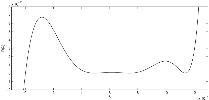
As an illustration, we show in Figure 2 a graph of the Evans function along the real axis for $\delta=3$, with the Fourier cut-off at $K=24$. We see that the Evans function has a zero at $\lambda=0$ and double zeros around $0.0005$, $0.0007$ and $0.0011$. The zero at $\lambda=0$ corresponds to the eigenvalue at the origin caused by translational symmetry. The other zeros correspond to double eigenvalues. They have positive real part and thus we can conclude that the planar wave is unstable for $\delta=3$—coinciding with the long-established statements in Section 5.

In fact, the zeros for the Evans function can be related to the dispersion curve in Figure 1. As mentioned above, the differential equation (14) decouples into $2K+1$ subsystems of the form (21), each corresponding to the linear operator ${\mathcal{L}}$ given in (20) for a particular wave number. The basis vectors we chose for the unstable subspace are zero for all but one of these subsystems. Since the subsystems are decoupled, the solution at $x=x_{*}$ is also zero for all but one of these subsystems. Thus, the matrix $\bigl{(}Y^{-}(x_{*};\lambda)\,\,Y^{+}(x_{*};\lambda)\bigr{)}$ at the matching point is (after reordering) a block-diagonal matrix consisting of $2K+1$ four-by-four blocks, and its determinant is the product of the determinants of the $4\times 4$ blocks. However, every determinant of a sub-block is the Evans function $D_{k}$ of the operator (20) for a particular wave number $k$. Thus, the Evans function for the two-dimensional planar wave is the product of the Evans functions for the one-dimensional wave with respect to transverse perturbations:

$$D(\lambda)=\prod_{k=-K}^{K}D_{k}(\lambda).$$ (24)

We chose $L=200$, so $k=1$ corresponds to a wave number of $\frac{2\pi}{200}\approx 0.0314$ in Figure 1. The plot shows that the corresponding growth rate is approximately 0.0005, thus $D_{1}(\lambda)$ has a zero around $\lambda=0.0005$. The dispersion relation is symmetric, so $D_{-1}(\lambda)$ has a zero at the same value. This explains why the two-dimensional Evans function has a double zero around $\lambda=0.0005$. Similarly, the double zeros around $\lambda=0.0011$ and $\lambda=0.0007$ correspond to $k=2$ and $k=3$, respectively.

As Figure 2 shows, the Evans function is of the order $10^{-60}$ in the interval of interest. It is important to emphasize that we are primarily interested in the zeros of the Evans function, which correspond to eigenvalues of the operator $\mathcal{L}$ defined in (10). The scale of the Evans function between the zeros, which depends on the normalization of the eigenvectors (22) and (23), is of lesser relevance in this context. However for completeness, we address this issue in Section 6.5.

6.3 The wrinkled front

Having established that our method works for planar fronts, we now turn to the wrinkled front. The most immediate problem is that of computing reliable steady wrinkled fronts. The procedure we used to do this is outlined as follows:

• The partial differential algebraic system (17) is solved on the computational domain $[-150,150]\times[-60,60]$ with a second-order finite element method on a grid of right triangles formed by dividing a grid of $300\times 240$ rectangles along their diagonals. We used the Finite Element package Comsol Multiphysics™ [8] which includes a version of the DAE solver daspk.

• To obtain reasonable starting waveform profiles for the partial differential algebraic system (17), we constructed the one-dimensional waveform, which we then swept out uniformly in the transverse direction.

• For travelling waves that appeared to be stable, we use the freezing method described in Section 4 to obtain good starting waveform profiles to initiate the use of Newton’s method in Comsol.

• For travelling waves that appeared to be unstable, we use simple parameter continuation (also using Comsol) starting with a (parametrically) nearby stable wave.

Figure 3 shows the front which results for $\delta=3$.

Fig. 3: The wrinkled front for $\delta=3$. The left panel shows the $u$ component and the right panel shows the $v$ component.

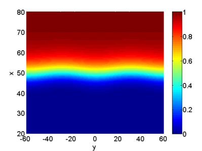
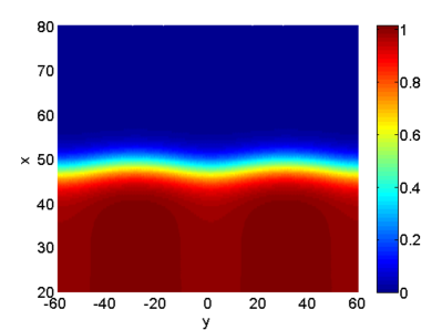
The wrinkled front varies along the transverse $y$-direction. Therefore, the Fourier coefficients ${\hat{D}}_{k}$ do not vanish for $k\neq 0$ and the differential equation (15) does not decouple. In the limits $x\to\pm\infty$, we have restricted ourselves to wrinkled front profiles that approach a $y$-independent state, which is the same as for the planar front. Hence, the computation of the stable and unstable subspaces for the planar front, which we reported above, remains valid for the wrinkled front.

Fig. 4: The Evans function along the real axis for the wrinkled front at $\delta=3$, computed using the Riccati approach. The three plots in the bottom row zoom in on the zeros of the Evans function.

Fig. 5: Same as Figure 4 but with the Drury–Oja approach.

The computation now proceeds as with the planar front. We solve the Riccati differential equation (4a) in the left and right intervals (as described in Section 6.1 above) for the Riccati approach, and (5) for the Drury–Oja approach. The front $U_{c}$ is determined as explained above, with interpolation being used for those points that fall between the grid points of the finite element solution. We use cubic interpolation, because linear interpolation is not sufficiently accurate. Finally, the Evans function is computed using either the modified form (8) or Humpherys and Zumbrun form (9).

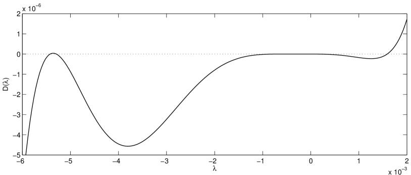
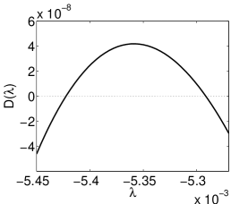
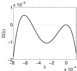
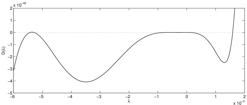
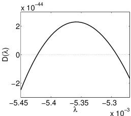
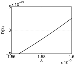
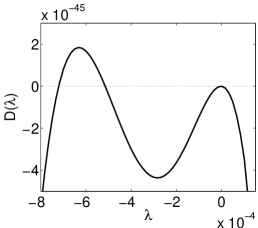
Figure 4 shows a plot of the Evans function along the real axis for $\delta=3$, computed using the Riccati approach. The result of the Drury–Oja approach is shown in Figure 5. For both approaches, we used projection on $K=9$ modes and we solved the Riccati differential equations (4a) (with appropriate coefficients for the left and right intervals), and the Drury–Oja equations (5), by the Matlab ODE-solver ode45 with absolute and relative tolerances of $10^{-8}$ and $10^{-6}$. The domain is $[-150,150]\times[-60,60]$ and as matching point we have chosen $x_{*}=50$ which is roughly the front location (see Figure 3). Both approaches produce Evans functions with zeros at (approximately) the same $\lambda$-values: there is one eigenvalue with a positive real part around $\lambda=0.0016$, a double zero around $0$ (due to translation invariance), and pairs of eigenvalues around $-0.0006$ and $-0.0053$. In particular, the eigenvalue around $\lambda=0.0016$ shows that the wrinkled front is unstable for $\delta=3$.

However, the Riccati and Drury–Oja approaches do differ in some respects. The Riccati approach involves integrating a system of half the dimension as compared to the Drury–Oja approach, so we can expect it to be faster, especially for large values of $K$ (in comparable experiments for large $K$, it was typically two to three times faster). See Ledoux, Malham and Thümmler [21] where some detailed accuracy versus cost comparisons can be found. We also note that the Drury–Oja approach again produced very small values for the Evans function, which as explained in Section 6.5, is not as alarming as it first seems. The Riccati approach, which uses a different scaling of the Evans function, yields only moderately small values, though again see Section 6.5.

We also used the angle between the unstable and stable subspace $\theta(\lambda;x_{\ast})$ to determine the location of the eigenvalues. Though this scales better than the Evans determinant, it is non-negative by definition and zeros occur as touch-downs in the complex spectral parameter plane. Actual zeros of the function are thus harder to establish compared to sign changes in the real and imaginary parts of the Evans determinant. Further, $\theta(\lambda;x_{\ast})$ is not analytic in $\lambda$.

$K$	Eigenvalues (Evans function)
3	$0.001609$	$-0.000026$	$-0.000781$	$-0.001296$	$-0.000670$	$-0.006078$	$-0.006177$
4	$0.001609$	$0.000002$	$-0.000001$	$-0.000519$	$-0.000670$	$-0.006078$	$-0.006177$
5	$0.001589$	$0.000002$	$-0.000001$	$-0.000519$	$-0.000720$	$-0.005295$	$-0.005426$
6	$0.001589$	$-0.000002$	$-0.000003$	$-0.000515$	$-0.000720$	$-0.005295$	$-0.005426$
7	$0.001589$	$-0.000002$	$-0.000003$	$-0.000515$	$-0.000721$	$-0.005292$	$-0.005422$
8	$0.001589$	$-0.000002$	$-0.000003$	$-0.000515$	$-0.000721$	$-0.005292$	$-0.005422$
9	$0.001589$	$-0.000002$	$-0.000003$	$-0.000515$	$-0.000721$	$-0.005292$	$-0.005422$
$\vdots$	$\vdots$
24	$0.001589$	$-0.000002$	$-0.000003$	$-0.000515$	$-0.000721$	$-0.005292$	$-0.005422$
	Eigenvalues (ARPACK)
	$0.001592$	$0.000000$	$0.000000$	$-0.000514$	$-0.000719$	$-0.005289$	$-0.005420$

Table 1: Zeros of the Evans function for the wrinkled front at $\delta=3$ for different values of the wave number cut-off $K$, as computed with the Riccati and Drury–Oja approaches. The last row shows the eigenvalues computed by ARPACK.

More accurate values for the zeros of the Evans function can be found by using a standard root-finding method. This yields the values listed in Table 1. The results of the Riccati and Drury–Oja approaches agree (to the precision shown) in all cases. The table also shows results for different values of the wave number cut-off $K$. The eigenvalues converge quickly when $K$ increases, and projection on $K=7$ modes is sufficient to get six digits of accuracy, at least in this example. The largest computation we performed is with $K=24$, in which case the one-dimensional equation has order $196$.

We also computed the eigenvalues by a projection method to check these results. The Comsol package, which we used to compute the travelling front, has an eigenvalue solver based on the Arnoldi method as implemented in ARPACK [22]. This solver uses a shift $\sigma$ to allow the user to choose on which part of the spectrum to concentrate. We found that the choice of this shift is not straightforward. It is unwise to use a shift which is exactly an eigenvalue, so in particular, the default value of $\sigma=0$ should not be used. We used a shift of $\sigma=1$ or $\sigma=3$ which proved to be safe. The resulting eigenvalues are also listed in Table 1. They are in close agreement with the eigenvalues found using the Evans function, giving additional confidence in our computation.

Fig. 6: The locus where the real and imaginary parts of Evans function vanish for the wrinkled front at $\delta=3$. This plot uses a $100\times 100$ grid in the depicted region of the complex plane. The Evans function was computed on the 5000 grid points in the top half and extended by symmetry to the bottom half.

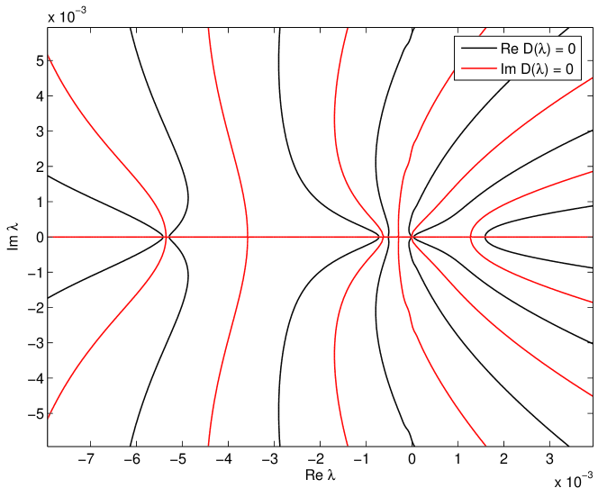
Figure 6 shows the contours where the real and imaginary parts are zero; eigenvalues correspond with the intersections of these contours. All eigenvalues are real. Interestingly, the contours are well separated on the boundary of the depicted region of the complex plane even though the eigenvalues are packed closely together. This suggests that it may be better to study the Evans function in a contour surrounding the eigenvalues instead of concentrating on the eigenvalues themselves—see Section 6.4.

Fig. 7: The Evans function along the real axis for the wrinkled front at $\delta=2.5$, computed using the Riccati approach. The right panel zooms in on the flat plateau around the origin in the left panel.

Fig. 8: Same as Figure 7 but with the Drury–Oja approach.

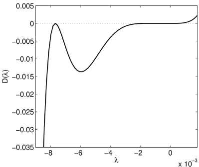
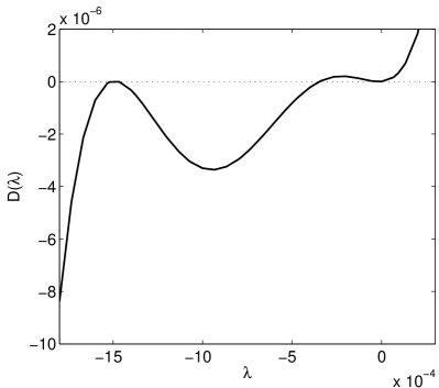
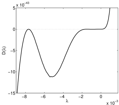
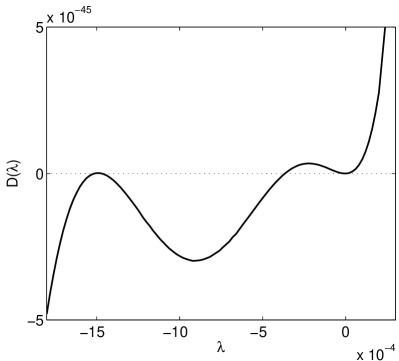
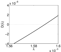
Figures 7 and 8 show the Evans function for the case $\delta=2.5$. The Evans function no longer has a zero with positive real part, meaning that there are no unstable eigenvalues. Hence for this value of $\delta$ the wrinkled front is in fact stable. We have thus established the following overall stability scenario for travelling wave solutions of the cubic autocatalysis problem. When $\delta$ is less than $\delta_{\mathrm{cr}}\approx 2.3$ planar travelling waves are stable to transverse perturbations. For $\delta$ beyond this instability there exist wrinkled fronts that are stable for $\delta=2.5$. However for $\delta=3$ these wrinkled fronts themselves become unstable. These stability results may depend on the transverse domain size (which we fixed at $L=120$); see Horváth, Petrov, Scott and Showalter [18].

6.4 Global eigenvalue search methods

If one is only interested in the stability of the underlying front then several methods exist to detect eigenvalues in the right-half complex spectral parameter plane—which also require relatively few Evans function evaluations. One important method uses the argument principle. We have the following sectorial estimate for the spectrum of ${\mathcal{L}}$: if $\lambda\in\sigma({\mathcal{L}})$ then

$$\mathrm{Re}(\lambda) \leq\|\mathrm{D}F(U_{c})\|_{L^{\infty}(\mathbb{R}\times\mathbb{T})},$$ (25a)

$$\mathrm{Re}(\lambda)+|\mathrm{Im}(\lambda)| \leq\frac{c^{2}}{4\kappa}+2\,\|\mathrm{D}F(U_{c})\|_{L^{\infty}(\mathbb{R}\times\mathbb{T})},$$ (25b)

where $\kappa\equiv\min\{B_{11},B_{22}\}$—we provide a proof in Appendix A. Hence we can restrict our search for unstable eigenvalues to the region of the complex $\lambda$-plane bounded by these inequalities.

In our case, we have $c\approx 0.577$ and $\|\mathrm{D}F(U_{c})\|_{L^{\infty}}\approx 1.422$ for $\delta=2.5$, and $c\approx 0.548$ and $\|\mathrm{D}F(U_{c})\|_{L^{\infty}}\approx 1.450$ for $\delta=3$. So, the above estimate implies that any eigenvalue $\lambda$ satisfies $\mathrm{Re}(\lambda)<1.5$ and $\mathrm{Re}(\lambda)+|\mathrm{Im}(\lambda)|<3$. Any unstable eigenvalue is thus inside the contour bounded by these lines and the imaginary axis; this contour is depicted in the left part of Figure 9 (the small semi-circle around the origin is to exclude the double eigenvalue at the origin, as explained below). The Evans function is analytic inside this contour, and thus we can count the number of zeros inside the contour by computing the change of the argument of the Evans function as $\lambda$ goes around the contour.

Fig. 9: The left figure shows the contour ${\mathcal{C}}$ in the complex plane. The right figure shows the argument of $D(\lambda)$ when $\lambda$ transverses the top half of this contour (for the wrinkled front with $\delta=3$). The plot is split up in four parts, corresponding to the quarter circle, the segment along the imaginary axis, the diagonal segment, and the segment going down. The scale on the horizontal axis is linear on the first, third and fourth part and logarithmic on the second part.

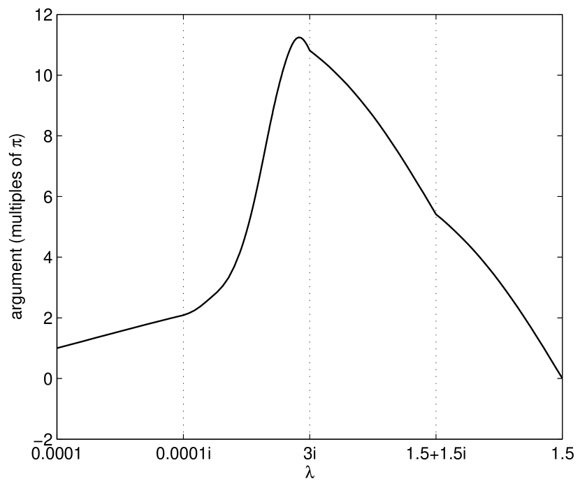
This suggests the following method. We divide the contour ${\mathcal{C}}$ in small segments, compute the Evans functions at the end points of the segments, find the change in the argument over each section and sum these to find the total change over the whole contour. The number of zeros is then the change of the argument divided by $2\pi$. The segments in which the contour is divided have to be chosen small enough that the change of the argument over each segment is smaller than $\pi$. Adaptive procedures to achieve this have been proposed by, amongst others, Ying and Katz [31], but for simplicity we determined the partition of the contour by trial and error.

The Evans function, with our choice of initial conditions, satisfies $D(\overline{\lambda})=\overline{D(\lambda)}$. Hence, it suffices to transverse half the contour ${\mathcal{C}}$. The plot at the right of Figure 9 shows how the argument of $D(\lambda)$ changes as $\lambda$ transverses the top half of the contour. We see that the change over the whole contour is $-2\pi$, and thus there is one zero inside the contour. This is the zero around $\lambda=0.0016$ shown in Figure 5; there are no other unstable eigenvalues.

The operator ${\mathcal{L}}$ is invariant under translations and hence it has two eigenvalues at $\lambda=0$. Thus, the Evans function is zero at $\lambda=0$ and its argument is undefined. For this reason, the contour ${\mathcal{C}}$ includes a small semi-circle of radius $10^{-4}$ to avoid the origin. It is of course possible that we miss some eigenvalues because of this deformation. To guard against this, we also compute the change in the argument of $D(\lambda)$ as $\lambda$ transverses a circle around the origin with radius $10^{-4}$. We find that the argument changes by $4\pi$ and hence the Evans function has two zeros inside the circle. This shows that we have not missed any eigenvalues by the deformation of ${\mathcal{C}}$ around the origin.

Another method is the parity-index argument (which we have not investigated here, but we include a description for completeness). To determine if there are eigenvalues on the positive real axis, we could use that

$$D(\lambda)\sim 2\delta^{-K-1/2},$$

as $\lambda\to+\infty$, as we prove in Appendix B. A change in sign of the Evans function along the real axis indicates an unstable eigenvalue. This can be exposed by comparing the sign of the Evans function in the asymptotic limit $\lambda\to+\infty$ to its sign elsewhere on the positive real axis, or the derivative or second derivative of the Evans function along the real axis evaluated at the origin. Note that to implement this technique we need to ensure the Evans function evaluated in the neighbourhood of the origin and that generating the asymptotic limit have been normalized, as far as their sign is concerned, in the same way. This may require keeping careful track of the the non-zero analytic multiples dropped in our definition of the modified Evans function, i.e. the normalization of the initial data, the scalar exponential factor and the determinants of $u_{-}$ and $u_{+}$ (which can be computed analytically in the asymptotic limit also).

6.5 Convergence of the Evans function

The results reported in Table 1 show that the values of $\lambda$ for which the Evans function $D(\lambda)$ is zero converge as $K\to\infty$. However they do not show how the Evans function scales for other values of $\lambda$ (not in the spectrum) as $K$ becomes large. We see in Figure 2 for the planar front, that in the domain of interest with $\lambda$ of order $10^{-4}$, the Evans function computed using the Drury–Oja approach with $K=24$, is of order $10^{-60}$. Similarly, for the wrinkled front, we see in Figures 5 and 8, also computed using the Drury–Oja approach with $K=9$, the scale of the Evans function is of order $10^{-45}$ for $\lambda$ of order $10^{-4}$. These small results we find for the Evans function—far smaller than machine precision—suggest that the computation might be inaccurate because of round-off error. This is not the case here. The solution of the Drury–Oja equation (5) does not contain such small numbers. They only appear when the determinant is computed at the matching point, which is a stable computation; see for example Higham [17, §13.5]. The determinant is computed by performing an LU-decomposition with partial pivoting and then multiplying the diagonal entries. Both steps are numerically stable even though the final result may be very small (as long as it does not underflow). The factorization (24) for the planar front provides another view point: the Evans function for $K=24$ is the product of $2K+1=49$ one-dimensional Evans functions, and if each of them is 0.06—not a very small number—then their product is of the order $10^{-60}$, which is a very small number.

For the modified Evans function we construct using the Riccati approach, we see in Figure 4, that in the domain of interest, it is of order $10^{-6}$ when $K=9$. If we reproduce Figure 4 for increasing values of $K$, we find that the modified Evans function actually grows. For large $K$, it increases roughly by a factor of $10$ per unit increase in $K$. However it is important to emphasize that the solutions to the Riccati systems, that are used to construct the modified Evans function, remain bounded. It is only when we evaluate the determinant, that for example when $K=21$, the scale of the modified Evans function in Figure 4 is of order $10^{4}$. Hence the question of the scaling of the Evans function comes into play in the multi-dimensional context.

In the one-dimensional case, the standard definition of the Evans function is (7) given in Alexander, Gardner and Jones [1]. Of course this definition stands modulo any analytic non-zero multiplicative factor—afterall it’s the zeros of the Evans function we are typically after. A different appropriate normalization of the initial data $Y_{0}^{\pm}(\lambda)$ rescales the Evans function by such a factor. Further it is common to drop the scalar exponential factor. Hence for example the difference between the Humpherys and Zumbrun Evans function (9) and the standard Evans function is that the scalar exponential factor is dropped and the initial data might be normalized differently when it is $QR$-factorized. For the modified Evans function in (8), we dropped the exponential factor and also the determinants of some full rank submatrices in the determinant of the standard Evans function.

However such analytic non-zero factors impact the scale of the Evans function in the multi-dimensional context, as they depend on $K$. This can lead to growth or decay of the Evans function employed away from the eigenvalues as $K$ is increased, depending on which factors are kept and which are dropped. This is precisely what we have observed for the Drury–Oja and Riccati approaches, which decay and grow, respectively, as $K$ increases.

Gesztesy, Latushkin and Zumbrun [12, §4.1.4] show that the Evans function, when suitably normalized, coincides with the 2-modified Fredholm determinant of a certain operator related to ${\mathcal{L}}$. Importantly, the 2-modified Fredholm determinant converges as $K\to\infty$. They treat the self-adjoint case; the non-self-adjoint operator ${\mathcal{L}}$ we consider can, using suitable exponential weight functions, be transformed into a self-adjoint one (numerically though this is not necessary and could introduce further complications due to the introduction of exponential factors in the potential term). Gesztesy, Latushkin and Zumbrun define the Evans function much like we have, through a Galerkin approximation, using the matching condition (7). Their normalization, natural to their context, involves ensuring the Evans function does not depend on the coordinate system chosen and is invariant to similarity transformations (see Gesztesy, Latushkin and Makarov [11]). Crucially, Gesztesy, Latushkin and Zumbrun demonstrate in Theorem 4.15 that their 2-modified Fredholm determinant equals the Evans function multiplied by an exponential factor (nonzero and analytic), whose exponent diverges as $K\to\infty$ (it can diverge to positive or negative infinity depending on the precise form of the coefficient matrix $A(x;\lambda)$). Hence their Evans function diverges as well. Consequently, the 2-modified Fredholm determinant is a natural candidate for the canonical Evans function.

With this in mind, our observation regarding the measured divergence of the modified and Humpherys and Zumbrun Evans functions in our experiments, is not too surprising. Their divergence, the modified Evans function to large values, and the Humpherys and Zumbrun Evans function to small values, is simply a reflection of the over/under estimate of the crucial, correct multiplicative exponential factor that equates these Evans functions with the 2-modified Fredholm determinant of Gesztesy, Latushkin and Zumbrun, which guarantees a finite limit as $K\to\infty$. It would be interesting to see whether one can explicitly compute the factor relating the Evans function of Gesztesy, Latushkin and Makarov and the Evans function, as defined in this paper.

7 Concluding remarks

Our goal in this paper was to show, for the first time, that spectral shooting methods can be extended to study the stability of genuinely multi-dimensional travelling fronts. It was already obvious to the people working in this field that this can be done by a Fourier decomposition in the transverse dimension, thus reducing the problem to a large one-dimensional problem; however, no-one had yet managed to tackle the resulting large one-dimensional problems. This issue was overcome in theory by the work of Humpherys and Zumbrun [19] and latterly that of Ledoux, Malham and Thümmler [21], which showed that enough information for matching can be retained by integrating along the natural underlying Grassmannian manifolds (though these ideas have been well known in the control theory and quantum chemistry for a long while—see for example Hermann and Martin [16] and Johnson [20]). The dimension of the Grassmannian manifolds scale with the square of the order of the original problem. These methods brought the possibility of multi-dimensional shooting within our grasp, but there were still challenges to be overcome. We have addressed the most immediate of these in this paper:

1. How to project the problem onto the finite transverse Fourier basis and ensure a numerically well-posed large system of linear ordinary differential spectral equations;

2. How to construct the genuinely multi-dimensional fronts, this was a particular challenge which we managed to overcome using the combined techniques of freezing and parameter continuation (the latter for the unstable multi-dimensional fronts);

3. Choose a non-trivial but well-known example problem, which exhibits the development of planar front instabilities (an important initial testing ground for us) but also two-dimensional wrinkled fronts that themselves became unstable as a physical parameter was varied;

4. Apply the Humpherys and Zumbrun continuous orthogonalization as well as the Riccati methods to study the stability of the wrinkled fronts, in particular integrating a large system of order $196$—using $K=24$ transverse modes—hitherto the largest system considered in Evans function calculations was of order $6$ (see Allen and Bridges [2]).

5. Ultimately demonstrating the feasibility, accuracy, numerical convergence and robustness of multi-dimensional shooting to determine eigenvalues.

However there is still more to do. Though multi-dimensional shooting is competitive in terms of accuracy, how does it compare in terms of computational cost? There are multiple sources of error including: approximation of the underlying wrinkled front, domain truncation, transverse Fourier subspace finite projection, approximation of the solution to the projected one-dimensional spectral equations and the matching position. Our experience is that the accuracy of the underlying wrinkled front is especially important. Although we have endeavoured to keep all these errors small, not only for additional confidence in our numerical results, but also for optimal efficiency, we would like to know the relative influence of each one of these sources of error in order to target our computational effort more effectively. Finally we would also like to see how the method transfers to hyperbolic travelling waves and more complicated mixed partial differential systems.

Appendix A Sectorial estimate on the spectrum

We follow the standard arguments that prove that the parabolic linear operator $\mathcal{L}$ is sectorial, see for example Brin [5, p. 26]. First consider the $L^{2}$ complex inner product with the spectral problem

$$B\,\Delta U+c\partial_{x}U+\mathrm{D}F(U_{c})\,U=\lambda U.$$

Premultiplying this spectral equation with $U^{\dagger}$, and integrating over the domain $\mathbb{R}\times\mathbb{T}$, we get

$$-\int_{\mathbb{R}\times\mathbb{T}}\nabla U^{\dagger}B\nabla U\,\mathrm{d}x\mathrm{d}y+c\int_{\mathbb{R}\times\mathbb{T}}U^{\dagger}\,\partial_{x}U+U^{\dagger}\,\mathrm{D}F(U_{c})\,U\,\mathrm{d}x\mathrm{d}y=\lambda\|U\|_{L^{2}}^{2}.$$

In this last equation, if we set $B=P^{\mathrm{T}}P$ where $P\equiv\mathrm{diag}\bigl{\{}B_{11}^{1/2},~{}B_{22}^{1/2}\bigr{\}}$, we get

$$\lambda\|U\|_{L^{2}}^{2}+\|P\nabla U\|_{L^{2}}^{2}=c\int_{\mathbb{R}\times\mathbb{T}}U^{\dagger}\,\partial_{x}U+U^{\dagger}\,\mathrm{D}F(U_{c})\,U\,\mathrm{d}x\mathrm{d}y.$$ (26)

If we consider the complex conjugate transpose of the spectral equation, postmultiply with $U$, and integrate over the domain $\mathbb{R}\times\mathbb{T}$, we get

$$\bar{\lambda}\|U\|_{L^{2}}^{2}+\|P\nabla U\|_{L^{2}}^{2}=c\int_{\mathbb{R}\times\mathbb{T}}\partial_{x}U^{\dagger}\,U+U^{\dagger}\,\bigl{(}\mathrm{D}F(U_{c})\bigr{)}^{\mathrm{T}}\,U\,\mathrm{d}x\mathrm{d}y.$$

If we now add these last two equations then we get

$$\mathrm{Re}(\lambda)\|U\|_{L^{2}}^{2}+\|P\nabla U\|_{L^{2}}^{2}= \;\int_{\mathbb{R}\times\mathbb{T}}U^{\dagger}\,\tfrac{1}{2}\bigl{(}\mathrm{D}F+(\mathrm{D}F)^{\mathrm{T}}\bigr{)}(U_{c})\,U\,\mathrm{d}x\mathrm{d}y$$

$$\leq \;\|\mathrm{D}F(U_{c})\|_{L^{\infty}}\|U\|_{L^{2}}^{2}.$$ (27)

Now dividing through by $\|U\|_{L^{2}}^{2}$ we get (25a)

Next consider taking the imaginary part of (26) followed by the absolute value on both sides and using Hölder’s inequality to get

$$|\mathrm{Im}(\lambda)|\,\|U\|_{L^{2}}^{2}\leq c\|U\|_{L^{2}}\|\nabla U\|_{L^{2}}+\|\mathrm{D}F(U_{c})\|_{L^{\infty}}\|U\|_{L^{2}}^{2}.$$ (28)

Adding inequalities (27) and (28) and using that $\|P\nabla U\|_{L^{2}}^{2}\geq\kappa\,\|\nabla U\|_{L^{2}}^{2}$, where $\kappa\equiv\min\{B_{11},B_{22}\}$, and the arithmetic-geometric mean inequality

$$c\|U\|_{L^{2}}\|\nabla U\|_{L^{2}}\leq\frac{c^{2}}{4\kappa}\|U\|_{L^{2}}^{2}+\kappa\|\nabla U\|_{L^{2}}^{2},$$

we get (25b)—after dividing through by $\|U\|_{L^{2}}^{2}$.

Appendix B Evans function when spectral parameter is large

We follow the arguments for such results given in Alexander, Gardner and Jones [1, p. 186] and Sandstede [25, p. 24]. We begin by rescaling $\tilde{x}=\sqrt{|\lambda|}\,x$ in (14) for each $k=-K,-K+1,\ldots,K$ and taking the limit $|\lambda|\rightarrow\infty$ to get

$$\partial_{\tilde{x}\tilde{x}}{\hat{U}}_{k}-\mathrm{e}^{\mathrm{i}\,\mathrm{arg}\lambda}B^{-1}{\hat{U}}_{k}=0.$$

Hence we have a decoupled system of $2K+1$ equations of the form

$$\partial_{\tilde{x}}\begin{pmatrix}{\hat{U}}\\ {\hat{P}}\end{pmatrix}=\begin{pmatrix}O_{2(2K+1)}&I_{2}\otimes I_{2K+1}\\ \tilde{B}\otimes I_{2K+1}&O_{2(2K+1)}\end{pmatrix}\begin{pmatrix}{\hat{U}}\\ {\hat{P}}\end{pmatrix}$$

where $\tilde{B}=\mathrm{e}^{\mathrm{i}\,\mathrm{arg}\lambda}B^{-1}$. This is a constant coefficient linear problem and the so-called spatial eigenvalues $\mu$ are the roots of the characteristic polynomial

$$\mathrm{det}\bigl{(}(\mu^{2}I-\tilde{B})\otimes I_{2K+1}\bigr{)}=\bigl{(}\mathrm{det}(\mu^{2}I-\tilde{B})\bigr{)}^{2K+1}.$$

where for any matrix $C$ we have used that $\mathrm{det}\bigl{(}C\otimes I_{k}\bigr{)}\equiv\mathrm{det}\bigl{(}C^{k}\bigr{)}\equiv\bigl{(}\mathrm{det}\,C\bigr{)}^{k}$. Hence the spatial eigenvalues are $\pm\sqrt{B_{11}}$, $\pm\sqrt{B_{22}}$; each with algebraic multiplicity $2K+1$. Associated with each of these four basic spatial eigenvalue forms we have the $(2K+1)$-dimensional eigenspaces:

$$\mu=+\sqrt{B_{11}}\colon \quad\mathrm{span}\{e_{2k}^{+}(+\sqrt{B_{11}})\colon k=-K,-K+1,\ldots,+K\},$$

$$\mu=-\sqrt{B_{11}}\colon \quad\mathrm{span}\{e_{2k}^{-}(-\sqrt{B_{11}})\colon k=-K,-K+1,\ldots,+K\},$$

$$\mu=+\sqrt{B_{22}}\colon \quad\mathrm{span}\{e_{2k+1}^{+}(+\sqrt{B_{22}})\colon k=-K,-K+1,\ldots,+K\},$$

$$\mu=-\sqrt{B_{22}}\colon \quad\mathrm{span}\{e_{2k+1}^{-}(-\sqrt{B_{22}})\colon k=-K,-K+1,\ldots,+K\},$$

where $e_{i}(\beta)$ is the vector with $1$ in position $i$, with $\beta$ in position $2(2K+1)+i$, and zeros elsewhere. Hence as $|\lambda|\rightarrow\infty$, the Evans function has the asymptotic form

$$D(\lambda)\sim \;\mathrm{det}\begin{pmatrix}I_{2}\otimes I_{2K+1}&-I_{2}\otimes I_{2K+1}\\ \tilde{B}^{1/2}\otimes I_{2K+1}&\tilde{B}^{1/2}\otimes I_{2K+1}\end{pmatrix}$$

$$= \;2\,\mathrm{det}\bigl{(}\tilde{B}^{1/2}\otimes I_{2K+1}\bigr{)}$$

$$= \;2\,\bigl{(}\delta^{-1/2}\mathrm{e}^{\mathrm{i}\,\mathrm{arg}\lambda}\bigr{)}^{2K+1}.$$

References

- [1] J.C. Alexander, R. Gardner, and C.K.R.T. Jones, A topological invariant arising in the stability analysis of traveling waves, J. Reine Angew. Math. 410 (1990), pp. 167–212.
- [2] L. Allen and T.J. Bridges, Numerical exterior algebra and the compound matrix method, Numer. Math. 92(2) (2002), pp. 131–149.
- [3] N.J. Balmforth, R.V. Craster and S.J.A. Malham, Unsteady fronts in an autocatalytic system, Proc. R. Soc. Lond A. 455 (1999), pp. 1401–1433.
- [4] J. Billingham and D. Needham, The development of travelling waves in quadratic and cubic autocatalysis with unequal diffusion rates, I and II, Phil. Trans. R. Soc. Lond. A, 334 (1991), pp. 1–124, and 336 (1991), pp. 497–539.
- [5] L.Q. Brin, Numerical testing of the stability of viscous shock waves, PhD thesis, Indiana University, Bloomington, 1998.
- [6] W.-J. Beyn and V. Thümmler. Freezing solutions of equivariant evolution equations, SIAM J. Appl. Dyn. Syst., 3(2) (2004), pp. 85–116.
- [7] Å. Björck and G.H. Golub, Numerical methods for computing angles between linear subspaces, Math. Comp. 27(123) (1973), pp. 579–594.
- [8] Comsol Multiphysics 3.3, 2007. Comsol Inc., www.comsol.com.
- [9] J. Deng and S. Nii, Infinite-dimensional Evans function theory for elliptic eigenvalue problems in a channel, J. Differential Equations 225 (2006), pp. 57–89.
- [10] J.W. Evans, Nerve axon equations, IV: The stable and unstable impulse, Indiana Univ. Math. J. 24 (1975), pp. 1169–1190.
- [11] F. Gesztesy, Y. Latushkin and K.A. Makarov, Evans functions, Jost functions, and Fredholm determinants, Arch. Rational Mech. Anal. 186 (2007), pp. 361–421.
- [12] F. Gesztesy, Y. Latushkin and K. Zumbrun, Derivatives of (modified) Fredholm determinants and stability of standing and travelling waves, J. Math. Pures Appl. 90(2) (2008), pp. 160–200.
- [13] J. Greenberg and M. Marletta, Numerical solution of non-self-adjoint Sturm-Liouville problems and related systems, SIAM J. Numer. Anal. 38(6), pp. 1800–1845.
- [14] P. Griffiths and J. Harris,Principles of algebraic geometry, Wiley Classics Library Edition, 1994.
- [15] D. Henry, Geometric theory of semilinear parabolic equations, Lecture Notes in Mathematics 840, Springer–Verlag, 1981.
- [16] R. Hermann and C. Martin, Lie and Morse theory for periodic orbits of vector fields and matrix Riccati equations, I: general Lie-theoretic methods, Math. Systems Theory 15 (1982), pp. 277–284.
- [17] N. Higham, Accuracy and Stability of Numerical Algorithms, second edition, SIAM, 2002.
- [18] D. Horváth, V. Petrov, S.K. Scott and K. Showalter, Instabilities in propagating reaction-diffusion fronts, J. Chem. Phys. 98(8) (1993), pp. 6332–6343.
- [19] J. Humpherys and K. Zumbrun, An efficient shooting algorithm for Evans function calculations in large systems, Physica D 220 (2006), pp. 116–126.
- [20] B.R. Johnson, New numerical methods applied to solving the one-dimensional eigenvalue problem, The Journal of Chemical Physics 67(9) (1977), pp. 4086–4093.
- [21] V. Ledoux, S.J.A. Malham and V. Thümmler, Computing the Evans function using Grassmannians, submitted to Math. Comp., arXiv:0710.1037v2, 2 Sept 2008.
- [22] R.B. Lehoucq, D.C. Sorensen and C. Yang, ARPACK users guide: Solution of large scale eigenvalue problems with implicitly restarted Arnoldi methods, SIAM, Philadelphia (1998).
- [23] A. Malevanets, A. Careta and R. Kapral, Biscale chaos in propagating fronts, Phys. Rev. E 52 (1995), pp. 4724–4735.
- [24] J.W. Milnor and J.D. Stasheff, Characteristic classes, Annals of mathematics studies 76, Princeton University Press, 1974.
- [25] B. Sandstede, Stability of travelling waves, In Handbook of Dynamical Systems II, B. Fiedler, ed., Elsevier (2002), pp. 983–1055.
- [26] B. Sandstede and A. Scheel, Absolute and convective instabilities of waves on unbounded and large bounded domains, Physica D 145 (2000), pp. 233–277.
- [27] J. Schiff and S. Shnider, A natural approach to the numerical integration of Riccati differential equations, SIAM J. Numer. Anal. 36(5) (1999), pp. 1392–1413.
- [28] N. Steenrod, The topology of fibre bundles, Princeton University Press, 1951.
- [29] D. Terman, Stability of planar wave solutions to a combustion model, SIAM J. Math. Anal., 21 (1990), pp. 1139–1171.
- [30] V. Thümmler. Numerical analysis of the method of freezing traveling waves, PhD thesis, Bielefeld University, 2005.
- [31] X. Ying and I. Katz, A reliable argument principle algorithm to find the number of zeros of an analytic function in a bounded domain, Numerische Mathematik 53 (1988), pp. 143–163.