The role of advection in phase-separating binary liquids
Abstract
Using the advective Cahn–Hilliard equation as a model, we illuminate the role of advection in phase-separating binary liquids. The advecting velocity is either prescribed, or is determined by an evolution equation that accounts for the feedback of concentration gradients into the flow.
After obtaining some general results about the existence and regularity of solutions to the model equation, we focus on two specific cases: advection by a chaotic flow, and coupled Navier–Stokes Cahn–Hilliard equations in a thin geometry.
By numerically simulating chaotic flow, we show that it is possible to overwhelm the segregation by vigorous stirring, and to create a homogeneous state. We analyze the mixing properties of the model: by measuring fluctuations of the concentration away from its mean value, we find a priori bounds on the amount of homogenization achievable.
We discuss the Navier–Stokes Cahn–Hilliard equations and derive a thin-film version of these equations. We examine the dynamical coupling of the concentration and velocity (backreaction). To study long-time behaviour, we regularize the equations with a Van der Waals potential. We obtain existence and regularity results for the thin-film equations; the analysis also provides a nonzero lower bound for the film’s height, which prevents rupture.
We carry out numerical simulations of the thin-film equations and, by comparing the results with experiments on polymer blends, we show that our model captures the qualitative features of real binary liquids. The outcome of the phase separation depends strongly on the backreaction, which we demonstrate by applying a shear stress at the film’s surface. When the backreaction is small, the domain boundaries align with the direction of the stress, while for larger backreaction strengths, the domains align in the perpendicular direction.
Lastly, we compare and contrast the Cahn–Hilliard equation with other models of aggregation; this leads us to investigate the orientational Holm–Putkaradze model. We demonstrate the emergence of singular solutions in this system, which we interpret as the formation of magnetic particles. Using elementary dynamical systems arguments, we classify the interactions of these particles.
Acknowledgements
I would like to thank my supervisor Jean-Luc Thiffeault for his time, dedication, and fruitful exchanges in respect of this research. I am grateful to Darryl Holm for the introduction he gave me into Cahn–Hilliard dynamics. My other colleagues at Imperial College have always proved ready to answer my questions; in particular, I gratefully acknowledge the patience of Colin Cotter and Mark Haskins, and the generosity of Grigorios Pavliotis, who enthusiastically lent me what added up to be a significant fraction of his library.
I acknowledge the financial support of Imperial College and the effort of John Gibbons and Jean-Luc Thiffeault in arranging this. I am thankful for the additional support of the Government of Ireland through the Easter Week Scholarship scheme. The support of EPSRC through payment of research expenses is acknowledged.
I am grateful to my parents for their constant encouragement of my academic career and for their exhortations never to give up, and to Goodenough College, in whose safe confines in leafy Bloomsbury my wife and I stayed for the duration of my research. This leads me to thank my wife, Brooke, to whom I am indebted for her support and encouragement during my research, and for her general and great kindness.
Dedication
To my wife, Brooke: is duitse a scríobham an tráchtas seo, a stóirín.
Chapter 1 Introduction
Overview, review, preview
In her column in The Guardian, Maureen Lipman has depicted the routine of making home-made mayonnaise:
One day she… gave me a demonstration on how to make mayonnaise. I had no idea it was so technical… She whisked the mustard with one yolk for a few minutes, then started dribbling in the oil. As soon as any separation appeared she whisked even faster and continued whisking and oiling for long enough to make my wrist hurt, let alone hers. It was riveting, like watching an old master mixing his ochres with his burnt siennas. [1]
In this report we shall study this process in a more abstract setting, together with the parallel problem of phase separation in thin layers. We wish to characterize the competing effects of homogenization and phase separation in a stirred binary fluid. The advective Cahn–Hilliard equation describes precisely these mechanisms and this will be the subject of our report. In this chapter we shall review the literature pertaining to both stirred and unstirred phase separation under Cahn–Hilliard (CH) dynamics and then outline the study we have made.
In a seminal paper, Cahn and Hilliard [2] introduced their eponymous equation to model the dynamics of phase separation. They pictured a binary alloy in a mixed state, cooling below a critical temperature. This state is unstable to small perturbations so that fluctuations cause the alloy to separate into bubbles (or domains) rich in one material or the other. A small transition layer separates the bubbles. Because the evolution of the concentration field is an order-parameter equation, this description is completely general. Thus, by coupling the phase-separation model to fluid equations, one has a broad description of binary fluid flow encompassing polymers, immiscible binary fluids with interfacial tension, glasses, and mayonnaise.
In industrial applications, the components of a binary mixture often need to be mixed in a homogeneous state [3]. In that case, the coarsening tendency of multiphase fluids is undesirable. In this report we shall examine how a stirring flow affects this mixing process. We are interested in stirring not just to limit bubble growth, as is often effected with shear flows, but to break up the bubbles into a homogeneous mixture. We shall also examine the interplay between the concentration gradients and the fluid velocity, and shall find that this coupling effect can play an important role in the control of phase separation
We outline previous work for three increasing levels of complexity: CH in the absence of flow, passive CH with flow, and active CH with flow.
Cahn–Hilliard fluids without flow: There is a substantial literature that treats of the CH equation without flow. For a review, see [4]. The main physical feature of this simpler model is the existence of a single lengthscale (the bubble or domain size) such that quantities of interest (e.g., the correlation function) are self-similar under this scale. This length grows in time as , a result seen in many numerical simulations (see, for example, Zhu et al. [5]). Of mathematical interest are the existence of a Lyapunov functional, and hence of a bounded solution [6], and the failure of the maximum principle owing to fourth-order derivatives in the equation for the concentration field [7, 8].
Passive Cahn–Hilliard fluids: Given an externally-imposed flow (e.g., a shear flow, turbulence, or a stirring motion), we have a passive tracer equation for a CH fluid. There have been several studies of the (active and passive) shear-driven CH fluid [9, 10]. In these studies, it is claimed that domain elongation persists in a direction that asymptotically aligns with the flow direction, while domain formation is arrested in a direction perpendicular to this axis. This seems to be confirmed in the experiments of Hashimoto [11], although these results could be due to finite-size effects [12], in which the arrest of domain growth is due to the limitation of the boundary on domain size. Of interest is the existence or otherwise of an arrest scale and the dependence of this scale on the system parameters.
A more effective form of stirring involves chaotic flows, in which neighbouring particle trajectories separate exponentially in time, leading to chaotic advection [13]. The average rate of separation is the Lyapunov exponent, positive for such a flow [14, 15]. One may also regard this exponent as the average rate of strain of the flow. By imposing a chaotic flow on the CH fluid, finite-size effects are easily overcome. This is because the shear direction changes in time, so that domain elongation in one particular direction, leading to an eventual steady state in which domains touch many boundaries, is no longer possible. Berthier et al. [16] investigated the passive stirring of the CH fluid and observed a coarsening arrest arising from a dynamical balance of surface tension and advection. The stirring by the chaotic flow destroys large-scale structures, and this is balanced by the domain-forming tendency of the CH equation. A balancing scale is identified with the equilibrium domain size.
The importance of exponential stretching is amplified by the results of Lacasta et al. [17], in which a passive turbulent flow endowed with a tunable amplitude, correlation length, and correlation time, causes both arrest and indefinite growth, in different limits. We explain this heuristically as follows: In one limit of turbulent flow (small Prandtl number), velocity correlations are short in range compared to bubble size, fluid particles diffuse [18], and bubble radii evolve as , where is the bubble radius and is the effective tracer diffusivity. Because , the presence of diffusion fails to arrest bubble growth. In the limit of large Prandtl number however, the velocity field has long-range correlations and exhibits exponential separation of trajectories, so that the radius equation is , where is the average rate of strain, or Lyapunov exponent, of the flow. Thus, the exponential stretching due to stirring balances the bubble growth.
Active Cahn–Hilliard fluids: At the highest level of complexity, one considers the reaction of the mixture on the flow by coupling the CH equation to the Navier–Stokes equations. This choice of coupling is not unique, although the different models agree in the case that interests us, namely density-matched fluids [19, 20]. In experiments involving turbulent binary fluids near the critical temperature, it is found that a turbulent flow suppresses phase separation and homogenizes the fluid [21, 22]. However, by cooling the fluid further and maintaining the same level of forcing, phase separation is achieved. This result is limited to near-critical fluids, although it does suggest the possibility of homogenization by stirring in other contexts.
The most recent work on the CH fluid (Berti et al., [20]) focusses on the active CH tracer. They couple the CH concentration field to an externally-forced velocity field and observe coarsening arrest independently of finite-size effects. They identify a balance of local shears and surface tension as the mechanism for coarsening arrest. Thus, the chaotic advection discussed above is a sufficient condition for coarsening arrest, but not a necessary one since shear will suffice. Of interest again is the dependence of the arrest scale on the mean rate of shear.
With this literature in mind, we study the case of a chaotic flow coupled passively to the CH equation. Our ultimate focus will be on the breakup of bubbles by stirring, and not just coarsening arrest. We believe this aspect of CH flow deserves a further and more complete study, as it is a regime of particular relevance to industry, for example, in droplet breakup or in the mixing of polymers [23].
Berthier et al. [16] used an alternating sine flow to study coarsening arrest. Because of its simplicity, the sine flow is a popular testbed for studying chaotic mixing [24, 25, 26, 27, 28]. In contrast to Berthier et al. [16], we use a sine flow where the phase is randomized at each period, leading to a flow that has a positive Lyapunov exponent at all stirring amplitudes and for all initial conditions. This avoids the coexistence of regular and chaotic regions, which would lead to inhomeogeneous mixing characteristics over the domain of the problem. Because of its uniform stirring, the random-phase sine flow is often used as a proxy for turbulent stirring at high Prandtl number, but at much lower computational cost. Using this flow, we study coarsening arrest, as in previous papers [16, 20]. However, we shall also use it to study mixing due to the stirring and the hyperdiffusion of the CH dynamics. Under this additional process the scaling hypothesis that characterizes the dynamics of bubble formation, namely that there is one dominant lengthscale [4, 20], breaks down.
Having found a mechanism that counteracts domain formation and promotes mixing, we introduce a quantitative measure of homogenization, studying the power-mean fluctuation of the concentration about its average value. We specialize to the symmetric mixture in which equal amounts of both binary fluid components are present. By fluctuations about the average value, we mean spatial fluctuations around the (constant) average spatial concentration, which we then average over space and time. In effect, we study the time-averaged norm of the concentration. If this quantity is small, the average deviation of the system about the homogeneous state is small, and we therefore use this quantity as a proxy for the mixedness of the fluid. An approach similar to this has already been taken in the theory of miscible fluids [28, 29, 30, 31]. There, the equation of interest is the advection-diffusion equation, and fluctuations about the mean are measured by the variance or centred second power-mean of the fluid concentration [32, 33]. The variance is reduced by certain stirring mechanisms. By specifying a source term, it is possible to state the maximum amount by which a given flow can reduce the variance, and hence mix the fluid. By quantifying the variance reduction, one can classify flows according to how effective they are at mixing. Just as the linearity of the advection-diffusion equation suggested the variance as a natural way of measuring fluctuations in the concentration, the nonlinearity of the CH equation and its concomitant free energy (cubic and quartic in the concentration, respectively) will fix our attention on the fourth power-mean of the concentration fluctuations. Owing to Hölder’s inequality, a binary liquid that is well mixed in this sense will also be well mixed in the variance sense. The advantage we gain in considering the fourth power-mean is the derivation of explicit bounds on our chosen measure of mixedness, which have manifest flow- and source-dependence.
Due to the relevance of phase-separating thin films in industrial applications [3, 34], many experiments and numerical simulations focus on understanding how phase separation is altered if the binary fluid forms a thin layer on a substrate. One potential application of phase separation in thin films is in self-assembly [35, 36, 37]. Here molecules (usually residing in a thin layer) respond to an energy-minimization requirement by spontaneously forming large-scale structures. Equations of Cahn–Hilliard type have been proposed to explain the qualitative features of self-assembly [35, 38], and knowledge of variations in the film height could enhance these models. Therefore, we examine this application, and explain the main features of these studies, introducing a long-wavelength approximation of the coupled Navier–Stokes Cahn–Hilliard (NSCH) equations for a thin layer of fluid with a free surface.
Several recent experiments have clarified the different regimes of domain growth in a binary thin film. Wang and Composto [39] have identified early, intermediate, and late stages of evolution. The early stage comprises three-dimensional domain growth, while the intermediate stage is characterized by the formation of wetting layers at the film boundaries, the thinning of the middle layer, and significant surface roughening. Due to the thinning of the middle layer, the sandwich-like structure breaks up and matter from the wetting layer flows back into the bulk. Thus, a late stage is reached, consisting of bubbles coated by thin wetting layers. This characterization of the evolution has been seen in other experiments [40, 41, 42], although clearly a variety of behaviours is possible, depending on the wetting properties of the mixture. Our model captures the essential features of this evolution, in particular the tendency for concentration gradients to promote film rupture and surface roughening.
In a series of papers, Das et al. [43, 44, 45, 46, 47] numerically investigate the behaviour of binary fluids with wetting. In [43] they study the wetting properties of a binary mixture in an ultra-thin film. The behaviour is different from that in bulk mixtures. In bulk mixtures
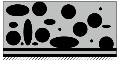
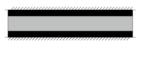
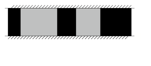
where one component of the binary fluid is preferentially attracted to the boundary, a layer rich in this component is established at the boundary, followed by a depletion layer. This layered structure propagates into the bulk and is called a spinodal wave [44, 45, 46]. In ultra-thin films, where the film thickness is less than a spinodal wavelength, this layered structure is suppressed. Two types of behaviour are then possible. In the partially wet case, both fluid components come into contact with the film boundaries. The ultimate state of the system is a domain-like structure extending in the lateral directions. The domains grow in time as , indicating Lifshitz–Slyozov diffusion [48]. In the other case, complete wetting, only one of the fluid components is in contact with the film boundaries. These different wetting regimes are portrayed schematically in Fig. 1.1. Our focus in this report is on the partially wet case.
The papers of Das et al. elucidate the role of wetting and film thickness on phase separation, although they do not discuss hydrodynamics or the effect of free-surface variations on domain formation. We therefore focus on ultra-thin films with a variable free surface, and for simplicity we restrict our attention to the case where both fluids experience the same interaction with the substrate and free surface. The model we introduce is based on the coupled NSCH equations. With an applied external forcing, the model highlights the effect of the dynamical backreaction of concentration gradients on the flow, a useful feature in applications where control of phase separation is required [37]. When the binary fluid forms a thin film on a substrate, a long-wavelength approximation simplifies the NSCH equations, which reduce to a pair of coupled evolution equations for the free surface and concentration. If is the scaled free-surface height, and is the binary fluid concentration, then the dimensionless equations take the form
| (1.1a) | |||
| where | |||
| (1.1b) | |||
| (1.1c) | |||
The symbol denotes the gradient operator in the lateral directions. The positive constants , , and measure surface tension, coupling strength between concentration and free-surface variations, and the scaled interfacial thickness, respectively. Additionally, is the dimensionless, spatially-varying surface tension, and is the body-force potential acting on the film. In this report we take , , the repulsive Van der Waals potential [49]. This choice stabilizes the film and prevents rupture. Although rupture is in itself an important feature in thin-film equations [50, 51, 52], in this report we are interested in late-time phase separation and it is therefore undesirable.
The analysis of thin-film equations was given great impetus by Bernis and Friedman in [53]. They focus on the basic thin-film equation
| (1.2) |
with no-flux boundary conditions on a line segment, and smooth nonnegative initial conditions. For this equation describes a thin bridge between two masses of fluid in a Hele–Shaw cell, for it is used in slip models as [54], while for it gives the evolution of the free surface of a thin film experiencing capillary forces [50]. Using a decaying free-energy functional, they prove the existence of nonnegative solutions to Eq. (1.2) for , while for , the solution is unique, strictly positive, and is almost always bounded in the norm. This paper has inspired other work on the subject [51, 52, 55], in which the effect of a Van der Waals term on Eq. (1.2) is investigated. These works provide results concerning regularity, long-time behaviour, and film rupture, in the presence of an attractive Van der Waals force. More relevant to the present work is the paper by Wieland and Garcke [56], in which a pair of partial differential equations describes the coupled evolution of free-surface variations, and surfactant concentration. The authors derive the relevant equations using the long-wavelength theory, obtain a decaying energy functional, and prove results concerning the existence and nonnegativity () of solutions. We shall take a similar approach in this report.
We have noted that equations of Cahn–Hilliard type have been used to model the self-assembly of molecules. In Ch. 7 we investigate the aggregation of magnetic particles using the Holm–Putkaradze model of aggregation. We compare and contrast the Holm–Putkaradze and the Cahn–Hilliard models. The formulation of these models through a gradient flow serves as a bridge between our study and more recent work in nanoscale modelling.
The modelling of nanoscale physics has become important in recent years, both because of industrial applications [57, 58, 59, 60], and because of the development of experiments that probe these small scales [61]. In a series of papers, Holm, Putkaradze and Tronci [62, 63, 64, 65, 66, 38] have focussed on the derivation of aggregation equations that possess emergent singular solutions. Continuum aggregation equations have been used to model gravitational collapse and the subsequent emergence of stars [67], the localization of biological populations [68, 69, 70], and the self-assembly of nanoparticles [35]. These are complexes of atoms or molecules that form mesoscale structures with particle-like behaviour. The utility of the Holm–Putkaradze model lies in its emphasis on nonlocal physics, and the emergence of singular solutions from smooth initial data. Because of the singular (delta-function) behaviour of the model, it is an appropriate way to describe the universal phenomena of aggregation and the subsequent formation of particle-like structures. Indeed in this framework, it is possible to prescribe the dynamics of the particle-like structures after collapse. Thus, the model provides a description of directed self-assembly in nanoscale physics [35, 36], wherein microscopic particles collapse under the potential they exert on each other, and form mesoscopic structures that in turn behave like particles. Our work in this area focusses on the vector-scalar Holm–Putkaradze model which, although derived elsewhere [62], has not yet been studied in any detail. This model provides an appropriate description of self-assembly of magnetic particles.
Although the Cahn–Hilliard theory has a venerable history, studies of phase separation with advection are more recent. Our result concerning homogenization by a chaotic flow is new. The application of (standard) functional analysis techniques to the advective Cahn–Hilliard equation, and the derivation of lower bounds on the amount of homogenization possible is also new. Although long-wavelength theory is common in applications, the thin-film Stokes Cahn–Hilliard (SCH) equations are entirely new, as are the numerical and analytical results concerning this model. In particular, we have identified a novel way of controlling phase separation by a combination of applied surface stresses and backreaction tuning. The vector Holm–Putkaradze model is a recent addition to the family of aggregation models and, while the equations were formulated elsewhere, our analysis of the coupled vector-scalar model is new.
This report is organized as follows. In Ch. 2 we derive the Cahn–Hilliard and Navier–Stokes Cahn–Hilliard equations from a combination of intuition and variational techniques. We discuss the elements of functional analysis that we need in this report, and prove an existence and uniqueness result for the CH equation with passive advection. In Ch. 3 we outline a numerical study of the CH equation stirred by a passive, chaotic flow. We characterize the mixing process by the lengthscales involved in the problem, by the concentration probability distribution function, and by a simple one-dimensional model. In Ch. 4, we use the functional analysis results of Ch. 2, and obtain upper and lower bounds on the level of mixedness achievable by any flow. In Ch. 5 we derive the thin-film Stokes Cahn–Hilliard equations, highlighting the importance of the dynamical coupling between the concentration and fluid velocity. We obtain existence and regularity results for the model equations. Although such analysis gives very precise results, it is unable to tell us much about the qualitative features of the solutions. Therefore, in Ch. 6 we carry out numerical simulations of the SCH equations, and compare the results with experimental papers. The simple model introduced here explains the qualitative features observed in real phase-separating fluids. In Ch. 7 we focus on the Holm–Putkaradze model of aggregation, which serves as a bridge between the Cahn–Hilliard model we have studied, and more recent work in nanoscale physics. We examine the equations introduced by Holm, Putkaradze, and Tronci for the aggregation of oriented particles [62, 63, 64, 65]. We investigate these equations numerically and study their evolution and aggregation properties. One aspect of nonlocal problems, already mentioned in [38], is the effect of competition between the lengthscales of nonlocality on the system evolution. We highlight this effect with a linear stability analysis of the full density-magnetization equations. Finally, in Ch. 8, we present our conclusions.
Publications
Many of the results presented in this thesis have already been published. We summarize this work in what follows. Unless otherwise stated, the principal author is L. Ó Náraigh and the co-author is J.-L. Thiffeault.
-
•
The numerical study of phase separation and passive chaotic advection is presented in [71].
-
•
The question, “given a passive flow in a binary liquid, by what amount can the fluid be homogenized?” is addressed in [72]. There, the authors use functional analytic and numerical techniques to answer this question.
-
•
Long-wavelength theory is used to derive a set of thin-film Stokes Cahn–Hilliard (SCH) equations in [73]. The authors highlight the importance of the backreaction when the control of phase separation is required.
-
•
Using a combination of numerical analysis and simple dynamical systems arguments, the vector Holm–Putkaradze model is investigated in [74]. The first author is D. D. Holm and the co-authors are L. Ó Náraigh and C. Tronci.
Statement of originality
The work presented in this thesis is my own, unless indication is given to the contrary.
Chapter 2 General Formulation
2.1 Overview
In this chapter we outline the thermodynamical formalism that gives rise to the Cahn–Hilliard equation and demonstrate its coupling to a flow field. We introduce the Navier–Stokes Cahn–Hilliard equations and obtain evolution equations for the physical quantities associated with the dynamical variables. We also discuss the mathematical formalism necessary to this report.
2.2 The Cahn–Hilliard equation
In this report, the Cahn–Hilliard model is viewed as an order-parameter equation, derived from thermodynamical considerations. An order-parameter description is independent of the detailed nature of the system being considered [75], and thus the equation is completely general, describing any two-component system where the mixed state is energetically unfavorable, and where the total amount of matter is conserved. Let be the order parameter, or simply put, the concentration of the binary fluid. We write down a free energy for the system in dimensions, as a functional of the concentration and temperature ,
| (2.1) |
where is a critical temperature, and where the gradient energy density penalizes the formation of sharp interfaces. Indeed, we shall see that the lengthscale represents the typical thickness of a smoothly-varying transition zone between unmixed regions, and that the finite thickness of these zones prevents the formation of infinite gradients in the problem. The constant appears in order to give Eq. (2.1) the correct units: has units of energy density. We shall, however, omit this constant if possible. The eager reader will note that Eq. (2.1) is nothing other than the Ginzburg–Landau free energy [75]. The system admits a critical temperature ; this is a threshold temperature across which the system exhibits qualitatively different behaviour. For , the energy density
has a single minimum at , and thus the mixed state is energetically favourable. On the other hand, for , the energy density has a double-well structure, with two stable minima at . These minima describe the pure phases of the mixture. The mixed state becomes a local maximum and is unstable (as the linear stability analysis in this section will demonstrate). We shall focus on the subcritical case, where spontaneous demixing is possible. Indeed, in the following derivation, we shall set , eliminating all thermal noise from the system. This simplification will be justified at the end of the derivation.
To minimize the free energy , the concentration evolves according to an equation of the type
where is an operator to be determined. Moreover, we are interested in conserved dynamics; that is, the total concentration must be constant. If, as in many applications [2], the system is invariant under changes of parity, the simplest form for the operator is,
where is a diffusion coefficient and is a nonnegative function called the mobility. The choice of mobility function is determined by physical considerations; for many of our applications, we shall simply set , while an in-depth discussion of the choice of functional form of is given in Sec. 3.7. Under these assumptions, the Cahn–Hilliard (CH) equation is
| (2.2) |
The order-parameter nature of this equation has resulted in its use in situations far beyond its original purpose as a model of the phase separation of a binary alloy [2]: it has found applications in polymer physics [23], in interfacial flows [19], and in mathematical biology [76]. By identifying the chemical potential [77] and the flux
| (2.3) |
the equation (2.2) can be recast in flux-conservative form:
so that, upon applying Gauss’s theorem, we have,
where is the problem domain in dimensions, is its boundary. The quantity is the differential element of area and is the outward-pointing unit normal. By specifying the boundary conditions (BCs)
| (2.4) |
the total concentration is conserved, and when combined with initial data, this gives sufficient information to solve Eq. (2.2).
We verify that the concentration evolution Eq. (2.2) causes the decay of free energy, as desired,
Using the BCs (2.4), this is simply
| (2.5) |
and the free energy is a decaying function of time.
Let us investigate the linear stability of a constant state . Performing a linear stability analysis of Eq. (2.2) about this state, we obtain an equation for the perturbation ,
and by making the ansatz , we obtain an expression for the growth rate of perturbations,
For , perturbations on scales below the critical lengthscale
decay, while perturbations on scales above grow. If the initial data contain a spectrum of lengthscales, this stability analysis demonstrates that small scales decay in amplitude, while large scales grow, suggesting the formation of large-scale structures. In later chapters we shall see that this is indeed the case. This linear stability analysis yields another piece of information: if the box size of the problem is less than the critical scale , then no large-scale structures can form, and the perturbations always decay to zero. This is the statement that the problem dimensions are so small as to favour the hyperdiffusion of Eq. (2.2) over phase separation, a useful result to keep in mind when considering phase separating liquids in ultrathin films.
The existence of equilibrium solutions to the CH equation (2.2) is well known [78], and we provide the details here because they will be useful in the following chapters. It is known that the late-time solution is one of bubbles, for which , with transition regions of thickness separating these bubbles. It is possible to derive an equilibrium solution that describes these transition zones. We write down the equilibrium version of the Cahn–Hilliard equation,
Let us set up a coordinate system on the bubble boundary with coordinates both perpendicular and parallel to the boundary. If the bubble’s radius of curvature is large, as indeed it will be at late times, then the equilibrium CH equation reduces to
| (2.6) |
where is the coordinate perpendicular to the bubble interface (we discuss the effects of a finite radius of curvature in Sec. 3.6). The boundary conditions place a single isolated bubble () in a sea of negative concentration, . Thus, the boundary conditions at are , . Multiplying Eq. (2.6) by the integrating factor and using the boundary conditions, we obtain the equation
| (2.7) |
with solution
| (2.8) |
consistent with the given boundary conditions. Note that for , Eq. (2.8) becomes a step function, with delta-function first derivative. Such infinite gradients are undesirable in our work, and we shall therefore always take .
In dimensions, the surface tension is the free energy associated with the bubble interface, per unit interfacial area. That is,
Upon substitution of the solution (2.8), the surface tension reduces to . Thus, , and has the correct dimensions of surface tension.
Finally, since is the coordinate perpendicular to the interface, the gradient has the form , where is a unit vector perpendicular to the interface. Thus, it follows from Eq. (2.7) that
and the kinetic and potential energy densities are in equipartition near the transition region. Moreover, far from the transition region, , and thus local equipartition also holds in the bulk. Integration over the domain of the problem therefore yields equipartition of kinetic and potential energy.
We examine briefly the evolution equation at finite temperatures. At finite temperatures, we are forced to take into account thermal fluctuations in the concentration field. Equation (2.2) is modified by the addition of a noise term,
| (2.9a) | |||
| where is a white-noise term satisfying the relation | |||
| (2.9b) | |||
Equation (2.9b) is the Cahn–Hilliard–Cooke equation [79]. Bray [80] shows that the scaling laws that characterize phase separation are the same for the Cahn–Hilliard and Cahn–Hilliard–Cooke equations, and that temperature is thus an irrelevant variable, at least when discussing the asymptotic (i.e. as ) features of phase separation. We are therefore justified in ignoring it in this report.
2.3 The Navier–Stokes Cahn–Hilliard equations
Using a combination of variational principles and physical intuition, we obtain a multicomponent flow model that couples fluid velocities to a concentration field. This approach is based loosely on the work of Lowengrub and Truskinowsky [19].
Consider a two-component binary liquid, with components labelled by the index . In a small volume , the component occupies a volume , with . In the same way, if the volume has total mass , with the fluid component giving a contribution , then . We introduce the real mass density , in contrast to the apparent mass density . Then, , where is the volume fraction. That is, given the characteristic function , with if is in the phase and zero otherwise, we have
where . With this knowledge, we introduce the binary liquid density,
To obtain a more convenient expression for , we make use of the following expression for the volume fraction ,
where we have defined the mass fraction ,
Thus, we obtain two equations for ,
Eliminating between the equations, we obtain an expression for the density which depends on the mass fraction ,
| (2.10) |
This is the so-called simple-mixture equation. Note that the density so defined is equivalent to the identity .
Let be the velocity at which the component travels in the mixture. We require that the mass of each binary fluid component be conserved,
By identifying the mass-weighted velocity field
| (2.11) |
we obtain a conservation law for the mixture variables ,
| (2.12) |
In this report we focus on density-matched fluids, for which . Then the mixture density is simply
and thus the mass-conservation law (2.12) reduces to the incompressibility condition
| (2.13) |
Moreover, we postulate an evolution equation for the concentration (mass fraction) , independently of the analysis in Sec. 2.2,
| (2.14) |
where is a chemical potential to be determined, and is a constant with the dimensions .
To find the dynamics of the concentration and velocity fields, we momentarily set to zero, and assume that the concentration is in fact conserved; that is, it satisfies
In the Lagrangian picture of fluid mechanics, this expression has the form
where the partial derivative indicates time differentiation with respect to a fixed Lagrangian label , and where the fluid parcel with label has the velocity
We write down a Lagrangian for the fluid velocity and phase-separating concentration,
where , and is a Lagrangian label. The density is then given as the Jacobian
and the term is the Lagrangian multiplier that enforces the constant-density condition. The Lagrangian action is then
Following standard practice [81], stationarity of this action with respect to variations in the Lagrangian trajectories yields the equations of motion. The variations along trajectories take place at fixed Lagrangian label, and the variation in the density has the form
which follows from the constancy of along particle trajectories, . Moreover, the related variations in concentration have the form,
and hence
Throughout the report, unless indication is given to the contrary, we use the summation convention and sum over repeated indices.
Using these relations, we vary the action over particle trajectories , at fixed particle label. We choose variations that vanish at the end times and , and at the container boundary . Thus,
Using , we obtain the constraint . Then using the result , we obtain the equation of motion
Finally, the stationarity result gives the constraint
We rewrite the equations in Eulerian form,
By making the identification and restoring , we obtain the equations
| (2.15a) | |||
| (2.15b) | |||
| (2.15c) |
We observe that the Lagrange multiplier that enforces the constant density plays the role of the pressure in these equations. The Lagrange multiplier is not arbitrary: it is fixed by the equation
Finally, we model the effect of viscosity by adding a diffusion term to Eq. (2.15a), which gives rise to the following constant-density Navier–Stokes Cahn–Hilliard (NSCH) equations,
| (2.16a) | |||
| (2.16b) | |||
| (2.16c) |
where is the kinematic viscosity of the mixture. By specifying the viscosity term as we have done, we confine ourselves to Newtonian fluids. These equations possess an energy ,
which is dissipated according to the relation
We comment on the symmetries of Eq. (2.16c). By identifying a tensor
| (2.17) |
Eqs. (2.16c) can be rewritten as
| (2.18a) | |||
| (2.18b) | |||
| (2.18c) |
Choosing as in Sec. 2.2, this set of equations is manifestly invariant under the change , a symmetry present in the basic CH equation. The form of the tensor in Eq. (2.17) is essential for preserving this symmetry. One way to picture this symmetry is to imagine that the concentration describes a binary mixture of a red and a green fluid, with indicating a region of pure red (green). The invariance of the equations (2.18c) is the statement that a person with dichromatism can be trusted to perform experiments on the system. Furthermore, owing to the form of the tensor in Eq. (2.17), the equations (2.18c) are rotationally invariant. Indeed, Eqs. (2.18c) provide a simple model in which these symmetries hold, and this reasoning provides another route to obtaining model equations for advection and phase separation.
We note that the passive version of Eq. (2.18c) is obtained by setting the backreaction term in the tensor to zero. In this limit, it is possible to imagine the incompressible velocity field as being prescribed, and we consider the much simpler equation
where is a diffusion coefficient. We shall be concerned with this passive advection equation in Chapters 3 and 4.
2.4 Inequalities: Relations between function spaces
In this section we outline some of the basic tools necessary for the mathematical analysis of partial differential equations (PDEs). We shall study a periodic domain in , although these results require only that be compact with Lipschitz boundary . We consider classes of functions that form a vector space with respect to a given norm. By deriving inequalities for the norms, we shall obtain relations between the vector spaces of functions.
We study functions of type
The norm of the function is the number
| (2.19) |
provided the integral exists. If the integral does exist, we write . The set is closed under addition and scalar multiplication of functions and therefore forms a vector space. This closure result will be useful in Ch. 5. We also have the Sobolev norm of the function ,
| (2.20) |
provided the integrals exist. Here refers to the derivative
If the integrals in Eq. (2.20) exist we write . Again, it can be shown that forms a vector space, called the Sobolev space. Finally, for functions of the type
we introduce the norm
provided the integral exists. If the integral exists we write , and identify another function space, .
To make progress in deriving relations between these norms, we introduce the following inequalities for real numbers.
-
•
Triangle inequality. If and are real numbers, then
-
•
Young’s first inequality. If and are real numbers, and if is any positive number, then
Proof: Since the square of any real number is nonnegative,
and the result follows.
-
•
Young’s second inequality. If and are positve real numbers, and if satisfy , then
Proof: Using the string of identities
and the convexity of the exponential function, , for , we obtain, by identifying , ,
as required.
Using this knowledge, we prove some results for function spaces.
-
•
Hölder’s inequality. Let and , with and . Then
Proof: Without loss of generality, we shall prove the inequality for the case when . Then it suffices to show that . By Young’s second inequality,
Integration over the domain gives the required result.
-
•
Cauchy–Schwarz inequality. When in Hölder’s inequality, we have the result
-
•
Hölder’s inequality for , . If the function is in the class , that is, if
then Hölder’s inequality holds with and ,
-
•
Monotonicity of norms. By setting in Hölder’s inequality, and , where , we obtain the result
A function that is bounded in the sense is therefore bounded in the sense. Such a result is called a continuous embedding [82]. We write,
-
•
Minkowski’s inequality. Let . Then,
Proof: Using the triangle inequality, we have,
Applying Hölder’s inequality to this relation, we have,
and the result follows.
-
•
Poincaré’s inequality. Let the function be a smooth, square-integrable function on the periodic domain . Then we have the relation
where is the mean value of the function .
Proof: Let be a variable running over all values in . By Parseval’s identity, -
•
Gagliardo–Nirenberg–Sobolev inequality. Let the function be a mean-zero, smooth, square-integrable function on the periodic domain . Then for and and integers satisfying , there is a constant such that
where
and for in the interval
with the restriction that if is a nonnegative integer, then must equal .
Proof: The proof is given in [83]. -
•
Gagliardo–Nirenberg–Sobolev inequality (celebrated special case). Let the function be a smooth, square-integrable function on the periodic domain . For , , , , and
the Gagliardo–Nirenberg–Sobolev inequality reduces to
where is called the Sobolev conjugate of . Rewriting this
we have the embedding
Here and are constants that are independent of the function .
Using the Minkowski inequality, and the result
it follows that and are norms on the vector spaces and respectively. These normed vector spaces are, moreover, complete, and therefore form Banach spaces [84].
As a conclusion to this theory section, we provide a list nonstandard inequalities that will be vital in Ch. 5 in analyzing the thin-film Stokes Cahn–Hilliard equations in one spatial dimension.
-
•
Let be a periodic domain in and let belong to the class . Then the following inequality holds,
(2.21) Proof: Using the Fundamental Theorem of Calculus, we have
Let be the maximum of the function over the set . That is, the maximum value of is attained at . Then
Since this is true for any , by integrating over , we obtain the inequality
as required.
-
•
Let belong to the class . Then the following inequality holds,
(2.22) Proof: We have the identity , true for any function with periodic boundary conditions (in general, this identity is true when ). With Hölder’s inequality, this yields
Using the relation (2.21), this becomes
which is a quadratic inequality in , with solution
By sacrificing the sharpness of the bound, we obtain a simpler one,
as required.
We shall use some of this formalism in the next section in proving the existence and uniqueness of solutions for a given PDE.
2.5 Galerkin approximations
In this section we study the typical fourth-order partial differential equation
| (2.23) |
on the periodic domain in , although the discussion is equally valid for any smooth bounded domain together with appropriate boundary conditions. The function belongs to the class , for any . Although the equation that forms the subject of this report is nonlinear, the intuition we gain in analyzing the linear equation (2.23) will enable us to study the advective Cahn–Hilliard equation (3.1), and to prove the uniqueness result of Ch. 5.
We specify the initial condition
and introduce the pairing
| (2.24) |
The strategy we take in analyzing Eq. (2.23) is to define weak solutions, construct a sequence of approximate weak solutions, show that this sequence converges to a limit that we identify as the solution, and obtain uniqueness results for this construction.
-
•
A function satisfies Eq. (2.23) weakly on if the following integral identity holds,
(2.25) is a smooth periodic test function, and .
-
•
We construct approximate solutions of Eq. (2.23) as Galerkin sums,
(2.26) where the ’s are eigenfunctions of the Laplace operator on , with eigenvalues , and where is the constant eigenfunction. The set is a complete orthonormal basis with respect to the pairing (2.24). If the equation (2.23) has initial data
then the approximate solution is seeded with the initial data
and converges strongly to in the norm.
-
•
To obtain the ’s, we demand that the Galerkin approximation (2.26) satisfy the following weak form of the PDE,
(2.27) for . This is simply
where the ’s are given by the relation . In matrix form, this is
(2.28) where . In view of the boundedness of the operator , the right-hand side of this expression is globally Lipschitz in the vector , and thus local existence theory [85] guarantees that Eq. (2.28) has a unique solution that is Lipschitz continuous in time, in a small interval . Thus, we have prescribed in a small time-interval .
-
•
To continue this solution to another time interval , and thus to the whole interval , we must find a bound on that depends only on the initial data. To do this, let us first of all replace with in Eq. (2.27), and obtain
(2.29) where is an arbitrary positive constant that comes from Young’s first inequality. Hence,
We choose such that . Then,
(2.30) where the number depends only on the initial conditions, and on the time .
Additional bounds are obtained by replacing with in Eq. (2.27). Then we obtain the inequality
(2.31) where is an arbitrary positive constant that comes from Young’s first inequality. Choosing gives
(2.32) where the number depends only on the initial conditions, and on the time . Choosing gives
(2.33) -
•
The uniform bounds (2.30), (2.32), and (2.33) enable us to continue the approximate solution to the whole time interval . Moreover, a uniformly bounded (in ) sequence of functions contains a subsequence (still denoted by ) which converges weakly to a limit , in the following sense***A bounded sequence on a Hilbert space always has a weakly convergent subsequence. Moreover, for weak convergence on a Hilbert space, , we have .,
Since the bound (2.30) is independent of and , it holds in the limit ,
Thus, by Poincaré’s inequality, we have a hierarchy of weak convergence results,
Since the bounds we have obtained are independent of , we have the conditions , in addition to the fact that .
-
•
By multiplying the Galerkin weak solution
(2.34) by a function that vanishes at and integrating the result over time, using the limiting relation , we obtain the relation
(2.35) By superposition, we can replace by a smooth function . Then, taking to be a distribution on , we obtain the result
(2.36) which is Eq. (2.25)
-
•
Inspection of Eq. (2.25) shows that is in the class , for any smooth , and it is therefore continuous. It follows that , as required.
-
•
Extra regularity is obtained by replacing the function in Eq. (2.27) with . Then,
To characterize the solution further, we make use of the theory of semigroups [86]. Formally, a solution to the equation
can be written as
| (2.37) |
The object , is a map from the Banach space to itself, and possesses the semigroup property
If and if is in its arguments†††A weaker condition on the function will suffice: if is in space and Hölder continuous in time, then Eq. (2.37) is still the unique, strong solution of the equation (2.23). Relaxing the assumption on even further gives rise to a less smooth solution. , then it can be shown [86, 87] that the solution (2.37) is a unique, strong solution of the equation (2.23), and coincides with the solution constructed by the Galerkin approximation. Indeed, the semigroup equation (2.37) holds for , where is a function of its arguments. In this manner, we have obtained the unique, strong solution to the equation (2.23), which satisfies the prescribed initial conditions and belongs to the class
We shall use this result, and this method of constructing solutions, throughout this report.
2.6 A strong existence theory for the advective Cahn–Hilliard equation
In this section we shall prove that solutions to the equation
exist and are unique, once a sufficiently regular starting condition and velocity field are prescribed. We work on a periodic domain in , although this restriction can be lifted. We shall use the machinery developed in Secs. 2.4 and 2.5. We present this analysis for two reasons. Firstly, it is important to develop understanding of the basic advective Cahn–Hilliard equation before carrying out further numerical and analytical studies. Secondly, since the results of this section are a combination of old analysis of a new equation, this section serves as a bridge between the well-known material of this chapter, and the new results that follow. To our knowledge, no analysis of the advective Cahn–Hilliard equation (2.38) exists in the literature, although the proof presented here is similar to Elliott’s and Zheng’s [6] for the nonadvective case. The introduction of advection necessitates a new ingredient in the proof, which we provide in (2.42). We shall provide analysis of the long-time behaviour of Eq. (2.38) in Ch. 4. Here prove the following statement,
Given the advective Cahn–Hilliard equation
(2.38) defined on the periodic domain , where and are positive constants, where is bounded in space and time in the following sense,
and where the initial data are defined by the identity
there exists a unique strong solution to Eq. (2.38) that lives in the class
for any .
We begin by constructing a Galerkin approximation to the weak problem
| (2.39) |
where is a smooth function on . We form the Galerkin approximation
with initial data
where the ’s are the eigenfunctions of on the domain , with corresponding eigenvalues ; is the constant eigenfunction. The Galerkin approximation is then required to satisfy the equation
or in vector form,
| (2.40) |
where is the matrix
and thus exists (of course, any linear operator on a finite-dimensional vector space has finite norm). On the other hand, we have the totally symmetric tensor
which is bounded in sense that . It follows that the function is Lipschitz in the vector , and local existence theory then guarantees that a solution to Eq. (2.40) exists in a small time-interval .
Next, we obtain a uniform bound on . Testing the equation (2.39) with , we obtain,
where the last line makes use of Young’s first inequality with . Thus,
| (2.41) |
where .
Now we consider the Galerkin approximation
and the chemical potential , and replace the test function by . Thus,
or
where is the approximate free energy. We examine the term . The parts of that are powers of drop out of this expression, owing to the antisymmetry of the operator . We are left with
The quadratic form satisfies , which gives rise to the inequality
| (2.42) |
Hence,
where . Integration over time yields
and since and , it follows that
independently of the order of the Galerkin approximation .
The same integration yields
Since , independently of , we have the bound
independently of .
Hence, from the theory developed in Sec. 2.5, it follows that
-
•
, weakly in ;
-
•
.
We shall now prove that , and hence that . We shall work in dimension , although the generalization to dimensions and is straightforward. We multiply the advective Cahn–Hilliard equation (2.38) by and integrate over space, to obtain
Let us consider the terms on the right-hand side. The first term is
where is an arbitrary positive constant. The second term is
where we have used Young’s second inequality and the Gagliardo–Nirenberg–Sobolev inequality in one spatial dimension. In particular, we have used the following Gagliardo–Nirenberg–Sobolev estimates,
and
the procedure for obtaining these results is sketched in Sec. 2.4. The same approach, with appropriate Gagliardo–Nirenberg–Sobolev estimates, gives the necessary bounds in higher dimensions. Finally, the third term is
Choosing , and integrating over gives the inequality
A sufficient condition for the boundedness of , and is obtained when and . We require that
Then we have the bound
Owing to the -independence of these results we obtain further information about the regularity of the weak solution ,
-
•
,
-
•
.
It follows that , which paves the way for our key result. This result also holds in dimensions and .
We obtain our final result by rewriting the advective Cahn–Hilliard equation as
We have shown that the function resides in . Using the result of Sec. 2.5, it follows that the solution is in fact strong, unique, and belongs to the class
Although the results in this section hold for any finite time-interval , they tell us nothing about the late-time behaviour of the solution to Eq. (2.38). Indeed, the exponential-in-time bounds (2.41) are distinctly unhelpful in answering this question. In Ch. 4 we shall prove the existence of long-time averages of the free energy . Let us, however, take this existence on trust for now, and perform numerical simulations on Eq. (2.38) for the case where is a chaotic flow.
Chapter 3 Chaotic stirring of a Cahn–Hilliard fluid
3.1 Overview
In this chapter we study the advective Cahn–Hilliard (CH) equation
| (3.1) |
for the case where is a prescribed chaotic flow. We focus our attention on the symmetric mixture, in which equal amounts of both binary fluid components are present. This special case involves a wide range of phenomena [5, 11, 20, 88, 89] and we are therefore justified in considering it here. However, the results in this chapter do not depend on this assumption. By numerically simulating a chaotic flow by the random-phase sine map, we characterize the effects of chaotic flow on the late-time concentration morphology. The key tool in this study is the use of scaling laws derived from dimensional analysis.
3.2 Scaling laws for the advective Cahn–Hilliard equation
In this section we discuss the notion of dynamical equilibrium for the CH equation without flow in terms of the structure function. We then examine the lengthscales that arise in the presence of flow.
The CH equation without flow exhibits dynamical equilibrium in the following sense. Starting from a concentration field fluctuating around the unstable equilibrium , the late-time concentration field has properties that are time independent when lengths are measured in units of typical bubble size . Such properties include the structure function [90] which we now introduce. A measure of the correlation of concentration between neighbouring points, given in Fourier space, is the following:
| (3.2) |
where denotes the spatial average. We normalize this function and compute its spherical average to obtain the structure function
| (3.3) |
The spherical average any function is defined as
| (3.4) |
where is the element of solid angle in dimensions and is its integral. Thus is the spherical average of the Fourier coefficient . For a symmetric binary fluid , the structure function is simply the spherically-averaged power spectrum:
| (3.5) |
The dominant lengthscale is identified with the reciprocal of the most important -value, defined as the first moment of the distribution ,
| (3.6) |
Since the system we study is isotropic except on scales comparable to the size of the problem domain, this lengthscale is a measure of scale size in each spatial direction. That is, we have lost no information in performing the spherical average in Eq. (3.3). This lengthscale is in turn identified with the bubble size: . In two-dimensional simulations () it is found [5, 90] that while and depend on time, is a time-independent function with a single sharp maximum, confirming that the system is in dynamical equilibrium and that a dominant scale exists. Indeed, the growth law is obtained, in agreement with the evaporation-condensation picture of phase separation proposed by Lifshitz and Slyozov (LS exponent) [48].
We present some simple scaling arguments to reproduce the scaling law and to illuminate the effect of flow. For , the equilibrium solution of Eq. (3.1) is in domains, with small transition regions of width in between. Across these transition regions, it can be shown [19] that
where
| (3.7) |
is the surface tension and is the radius of curvature. Thus, if is a typical bubble size, that is, a length over which is constant, the chemical potential associated with the bubble is
| (3.8) |
Balancing terms in the Cahn–Hilliard equation , it follows that the time required for a bubble to grow to a size is , implying the LS growth law .
Now the CH free energy is the system energy owing to the presence of bubbles:
The surface tension is the free energy per unit area. A bubble carries free energy , where prefactors due to angular integration are omitted. The total free energy in the motionless case is then , where is the total number of bubbles. Because the system is isotropic and because there is a well-defined bubble size, we estimate by . The free energy then has the scale dependence , and using the growth law for the length we obtain the asymptotic free energy relation
| (3.9) |
By introducing the tracer variance
| (3.10) |
and restricting to a symmetric mixture , we identify , where is the volume occupied by bubbles. Since , it follows that
| (3.11) |
We shall verify these results in Section 3.5. Equation (3.11) will provide a useful measure of bubble size when a flow is imposed, since no assumption is made about the number of bubbles per unit volume. In a dynamical scaling regime, the lengthscales calculated from these energy considerations must agree with that computed from the first moment of the structure function, since there is only one lengthscale in such a regime [78].
Stirring a CH fluid introduces new lengthscales. The flow will alter the sharp power spectrum found above and so it may not be possible to extract definite scales from experiments or numerical simulations. We might expect further ambiguity of scales during a regime change (crossover), for example, as the bubbles are broken up and diffusion takes over. Nevertheless, for a given flow, it is possible to construct lengthscales from the system parameters. We shall impose a flow that is chaotic in the sense that nearby particle trajectories separate exponentially in time at a mean rate given by the Lyapunov exponent.
If the advection term and the surface tension term have the same order of magnitude in a chaotic flow, by balancing the terms and we obtain a scale
| (3.12) |
where is the Lyapunov exponent of the flow. Because the term gives an exponential amplification of gradients, the balance of segregation and hyperdiffusion in the term may be broken and hyperdiffusion may overcome segregration. This will happen on a scale given by the balance of the terms and ,
| (3.13) |
In this regime, we expect mixing owing to the presence of the advection and the (hyper) diffusion. Using Eqs. (3.7), (3.12) and (3.13), the crossover between the bubbly and the diffusive regimes takes place when . In the following sections we shall examine these scales and look for this crossover between bubbles and filaments, the latter being characteristic of mixing by advection-diffusion.
3.3 A model stirring flow
In order to run simulations at high resolution, we make use of the sine flow model (4.25) in two dimensions. We are interested in the following velocity field, defined on a square domain with periodic boundary conditions:
| (3.14) |
where and are phases that are randomized once during each flow period and the integer labels the period. We solve Eq. (3.1) with and without the flow (4.25) to investigate the scaling laws presented in Section 5.2.
Equation (3.1) is integrated by an operator splitting technique, in which a specialized advective step followed by a phase-separation step are performed at each iteration. The phase-separation step is the semi-implicit spectral algorithm proposed by Zhu et al. [5] for the case without flow. The semi-implicitness of the algorithm enables us to use a reasonably large timestep, while the spectral nature of the phase-separation step enables us to work at high resolution, namely gridpoints. By imposing the sine flow (4.25), we may use Pierrehumbert’s lattice method for advection [27, 24]. With the problem defined on a discrete grid, this method is exact for the advection step. The sine flow has the added advantage that its correlation length is of order of the box size , which is the largest scale in the problem. Thus, using the prediction of Lacasta et al. [17] explained in Ch. 1, we expect this velocity field to produce coarsening arrest even at very small stirring amplitudes. The parameters and in Eq. (3.1) are dimensional, and we therefore nondimensionalize the equation before undertaking numerical simulations. Let be a timescale associated with the velocity , let be the magnitude of , and finally, let be the box size. It is then possible to write down Eq. (2.2) using a nondimensional time and a nondimensional spatial variable ,
where is a dimensionless shape function, , , and where The quantity is identified with the ratio , being the ratio of the velocity timescale to the diffusion timescale. For ease of notation, we shall henceforth take to mean , and drop the primes from the nondimensionalized equation. Now the lattice method with its splitting of the advection and diffusion steps, is effective only when the spread of matter due to diffusion is much slower than the spread due to advection, that is, . We therefore set . We shall also set and . Following standard practice [20, 16], we choose , the gridsize.
3.4 The Lyapunov exponent for the sine map
Loosely speaking, the Lyapunov exponent for a flow is the flow’s mean rate of strain. Here we define the Lyapuov exponent exactly and compute it for the special case of the two-dimensional sine flow. We provide an asymptotic expressions for the exponent, in the limit of small and large stirring amplitudes.
The integral of the period-one sine flow (3.14) gives a map from the 2-torus to itself:
| (3.15) |
By studying this map we may compute the Lyapunov exponent of the flow (3.14). Here and are stirring parameters and and are phases that are randomized once per period. The chaoticity of this map is quantified by the function :
| (3.16) |
where is a two-vector of initial conditions, is the stirring parameter and is the matrix
| (3.17) |
with . In what follows, for brevity, let
Finally, let the angle brackets denote an ensemble average over all possible phase angles.
We study the function for particular values of . For example, by setting we arrive at an expression of type , and applying L’Hôpital’s rule we replace with
| (3.18) |
Thus,
| (3.19) |
The quantity is the Lyapunov exponent of the map. In general, is a monotone increasing function of (see for example, Finn and Ott [91]), so that is an upper bound for . This nonequality also indicates the importance of the order in which the averaging is performed.
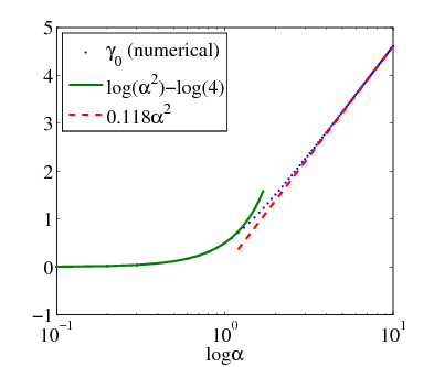
It is straightforward to compute : we obtain the exact result
| (3.20) |
where . The evaluation of is not so straighforward and so we have recourse to asymptotics. Thus, we replace the matrix by its large-amplitude approximation
where and . The quantity is easily calculated: it is
The order in which the computation is carried out is important: we take the log first and then ensemble average over all phase angles. Thus,
It remains to compute the phase average . We start with the last term and integrate over and first, since this is the only term depending on these variables. Hence,
or
We use the integral***For a derivation of this integral relation, see Appendix A.
to obtain the average , so that , and hence the result
| (3.21) |
The calculation in the limit is not as simple, and so we resort to numerical methods.
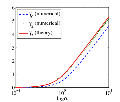
We compute numerically and compare the result with the theoretical prediction Eq. (3.20). Hereafter . We find that fluctuates noticeably compared with . It is systematically below the theoretical value. However, by increasing the number of realizations in the ensemble average, this difference disappears. These results are presented in Fig. 3.1. The reasonable agreement of the theory curve with the numerical one confirms the usefulness of the numerical calculation. Of significance is the fact that is nonnegative even for very small . Thus, the sine map is chaotic for all parameter values.
The large- result for is checked against a numerical simulation and a perfect agreement is obtained. In Section 3.5 we shall need a formula for the strain rate for moderate values of the stirring amplitude and so we fit a curve to for the parameter range . To make the system (1) invariant under , the fitted curve should be a polynomial in . The equation
| (3.22) |
is found to be optimal. Going to higher order in does not improve the accuracy of the fit.
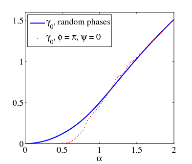
As a final computation we contrast the sine map with random phases with one in which the phases are constant and set to , . This contrast is shown in Fig. 3.1(c). For large , these maps have the same behaviour, growing as , and this is explained by the analysis of this section. For small there is an approximate parameter range for which the constant-phase map does not exhibit chaos. The asymptotic form is arrived at after 40 iterations for the random-phase map and after 10,000 iterations for the constant-phase map. Thus, in contrast to the constant-phase map, the random-phase map is efficient in separating trajectories at all stirring amplitudes and over all but very short timescales.
3.5 Numerical simulations
We integrate Eq. (3.1) in the manner explained in Sec. 3.3. The initial conditions are chosen to represent the sudden cooling of the binary fluid: above a certain temperature the homogeneous state is stable, while below this temperature the mixture free energy changes character to become , which makes the homogeneous state unstable. Thus, at temperatures , , and the sudden cooling of the system below leaves the system in this state. In order for the CH equation without thermal noise (3.1) to describe the evolution of these initial conditions, the cooling we have imposed must take the system to . Thus, we are working in the so-called deep-quench limit. With the initial conditions , both components of the fluid are present in equal amounts and the spatial average of the concentration field is zero.
Although the case without flow has been investigated before [5, 90], we reproduce it for two reasons. First, it serves as a validation of our algorithm. Second, we shall confirm the free energy laws (3.9) and (3.11) which to our knowledge have not been examined before. Finding an appropriate measure of bubble growth will be important for understanding the behaviour of the bubbles when we introduce stirring.
The results of these simulations are presented in Fig. 3.2. The scaling function is approximately time independent
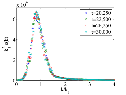
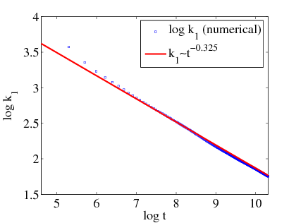
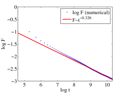
for as evidenced by Fig. 3.2(b), implying that the scaling exponents for and are to be extracted from the late-time data with . For finite-size effects spoil the scaling laws. Thus, while the scaling exponents are extracted from a small window, the fit is good and this suggests that the power laws obtained give the true time-dependence of and at late times. In this way we recover the dynamical scaling regime in which is time independent, in addition to the decay law [5]. Running the simulation repeatedly for an ensemble of random initial conditions improves the accuracy of the exponent. Furthermore, we obtain the energy laws , and . Thus,
| (3.23) |
so that , and all grow as and hence provide identical measures of scale growth, in agreement with the classical assumption that there is a unique lengthscale in the problem [4, 5].
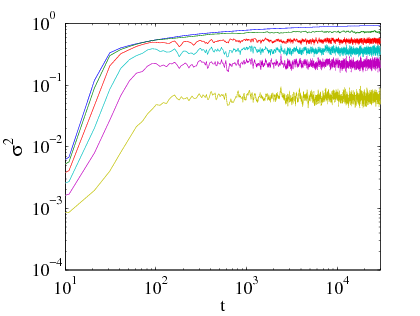
We investigate the stirred case in a similar manner and obtain the results below, after timesteps. In order to ensure that we are in a steady state, we study the inverse lengths and and the tracer variance (see Eq. (3.10)) which measures the homogeneity of the concentration ( for a homogeneous mixture) [24, 27]. These quantities are time dependent and have the property that after some transience, they fluctuate around a mean value, without secular trend. This can be seen in Fig. 3.3.
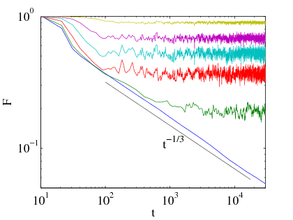
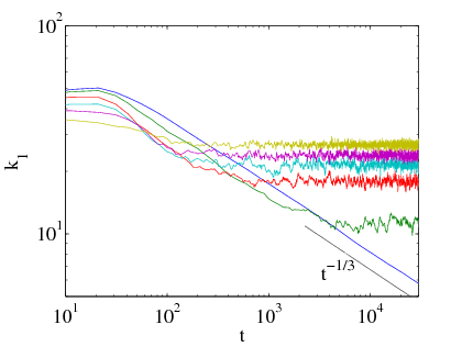
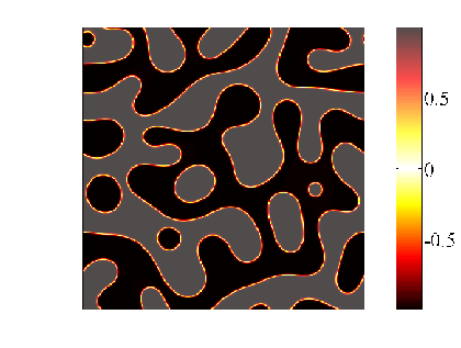
In Fig. 3.4, for , the concentration field at late time looks similar to that for . This is because for small , the effect of advection is diffusive, with small movements of particles
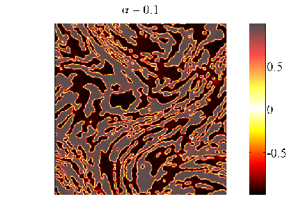
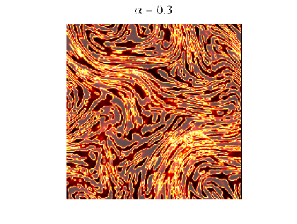
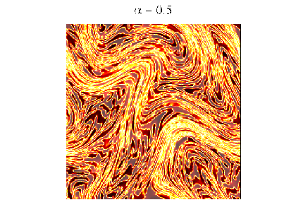
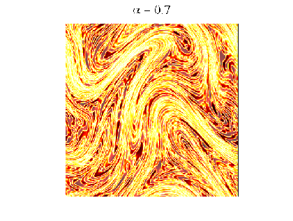
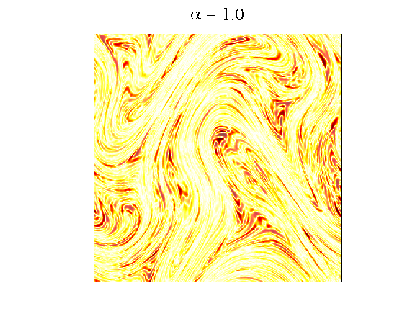
giving rise to bubbles with jagged boundaries, but no breakup. The PDFs of the concentration for have the same structure. Nevertheless, it is clear from Fig. 3.3(b) that coarsening arrest takes place for , in contrast to . As increases, the bubbles become less and less evident. For large , we see regions containing filaments of similar concentration. After a period of transience, the free energy , the mean wavenumber and the variance fluctuate around mean values, confirming the existence of the steady state. The bubble size is extracted from the quantity , where denotes a time average over the fluctuations. We investigate how the mean lengths scale with the Lyapunov exponent .
In Fig. 3.5 we see that for small the proxy for bubble radius scales with the
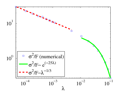
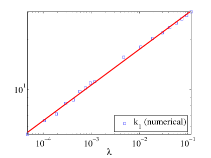
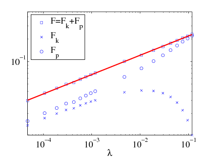
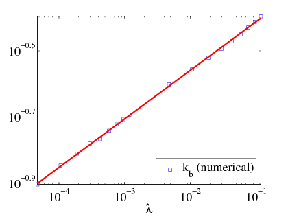
LS exponent as , suggesting an equilibrium bubble size on this scale. For larger , the hyperdiffusion breaks up these bubbles and mixes the fluid. This process leads to a faster-than-algebraic decay of bubble size, visible in the figure. Other measures of the bubble size, such as the mean wavenumber or the quantity do not possess a clear scaling law. For example, in Fig. 3.5(b) we plot against . The exponent changes over the three decades of data, indicating that the wavenumber does not have a clear scaling law with the Lyapunov exponent .
However, the dependence of the time-averaged free energy on the Lyapunov exponent has the power law behaviour over three decades, suggesting a genuine power law relationship. The time average of the Batchelor wavenumber [92] also possesses a clean power law over three decades.
In Sec. 2.2 we showed that in a situation of dynamical equilibrium characterized by a single lengthscale, the potential part of the free energy should be in equipartition with the kinetic part . In Fig. 3.5 we see that this is not the case when the bubbles start to break up as the stirring is increased. This is an indication of a crossover between the bubbly regime and the well-mixed one in which the variance is reduced by stirring.
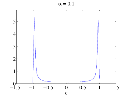
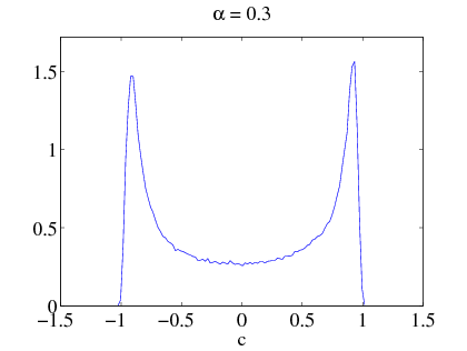
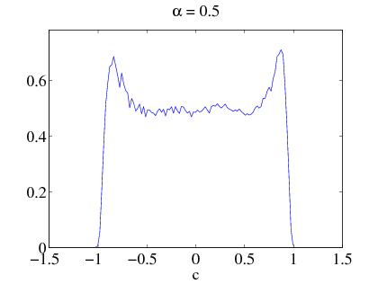
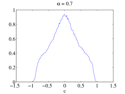
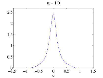
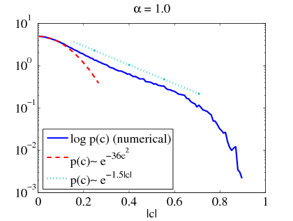
In Fig. 3.5 the breakdown in the power law relationship for large stirring amplitudes suggests a crossover between bubbly and diffusive regimes. Another way of seeing the transition between these regimes is to study the stationary probability distribution function (PDF) of the field . We do this in Fig. 3.6. For small values of we note that the PDF has sharp peaks at , indicating the effectiveness of phase separation at these stirring amplitudes. For however, the PDF has a Gaussian core, indicating that genuine mixing by advection-hyperdiffusion is taking place. For intermediate values of the PDF is a combination of these two different distributions of concentration.
3.6 A one-dimensional equilibrium problem
Having observed the crossover between the bubbly and the well-mixed regimes, we study a one-dimensional model to shed further light on the process by which this occurs.
We examine the archetypal hyperbolic flow , with strain rate . This flow tends to homogenize the concentration in the -direction through stretching. At late times the problem then becomes one dimensional:
| (3.24) |
Scaling lengths by and restricting to the steady case, Eq. (3.24) becomes
| (3.25) |
There are two sets of boundary conditions (BCs) that are of interest,
-
•
Bubble BCs: , , and .
-
•
Front BCs: , and .
The front solution has the interpretation of being the transition layer between filaments, the width of the layer giving the width of the filament. Before carrying out numerical work, we shall examine two asymptotic regimes where analytical progress is possible: the case without stirring, and that without phase separation.
No stirring
In the absence of advection () the model equation reduces to
| (3.26) |
which integrates to
| (3.27) |
where and are constants to be determined by the boundary conditions. We set bubble BCs , and . Using the bubble BCs and the requirement that the second derivative of should not diverge at infinity, is set to zero. Thus we have the Newton equation
| (3.28) |
By multiplying both sides by we obtain the energy relation
| (3.29) |
where we identify the potential energy and the total energy . The bubble boundary conditions then fix the values of and . The bubble or homoclinic solution is obtained when two roots of the equation coincide with one extremum of , given by
We pick out the homoclinic orbit by letting this extremum be at , giving . In addition, we specify the energy to be
Then in an interval , indicated in Fig. 3.7 (a), the energy exceeds , and , with equality at the interval boundary. Thus, the homoclinic solution is given by
By taking the reference level , we obtain the equation
| (3.30) |
Equation 3.30 specifies , which can then be obtained numerically, as in Fig. 3.7 (b).
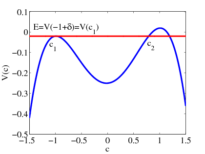
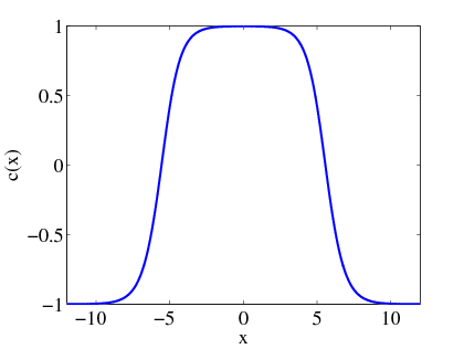
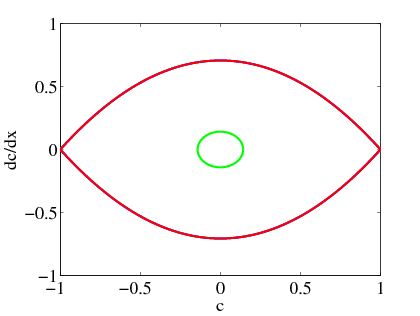
In the language of dynamical systems, the solution is a homoclinic orbit: the system returns to its initial state at after infinite time. The phase portrait of the solution is presented in Fig. 3.7(d).
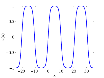
Finally we note that Eq. (3.28) possesses a host of different solutions, depending on the boundary conditions imposed. Let us take as before but leave the energy unspecified. We study the Newton equation , where is the potential . Periodic solutions exist when the system is placed in the potential well of Fig. 3.7 (a), and when . To obtain a solution with the flat peaks characteristic of a bubble, the system must access the anharmonic part of the potential, so we take . Thus the phase portrait of this periodic bubble solution almost coincides with the homoclinic orbit. On the other hand, for energies close to the well minimum the periodic solution is a small sinusoidal undulation. These results are best summarized by introducing the period of oscillation, given by [81]
where and are those roots of the equation indicated in Fig. 3.7 (a).
-
•
For the oscillations are small and the period is .
-
•
For the solution is still periodic with energy-dependent period. This is the one-dimensional gas of Fig. 3.7(c).
-
•
For , , giving the homoclinic solution.
-
•
For and , , which corresponds to the heteroclinic or front solution.
A quasi two-dimensional problem
Following the mechanical intuition developed in the previous section, we outline briefly what happens in the quasi one-dimensional setting when the full two-dimensional problem has azimuthal symmetry. In this case, the stationary CH equation is
where is the radial part of the Laplacian,
| (3.31) |
Using the same analysis as before, we obtain the equation , which is a Newton equation with damping:
| (3.32) |
where is the potential. The large-amplitude and homoclinic solutions presented previously are modified by the presence of damping: at small there is significant dissipation proportional to while the far-field problem is one of small oscillations
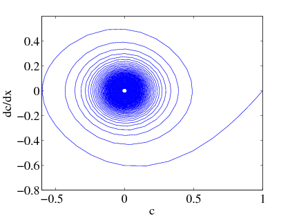
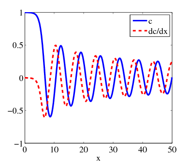
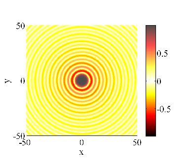
with damping. These oscillations have period ( is the well minimum), and decay to the attractor . These results are shown succinctly in the phase portrait of Fig. 3.8(a).
The no-segregation limit
By measuring lengths in terms of the diffusion lengthscale , Eq. (3.25) becomes
| (3.33) |
which in the limit of large reduces to
| (3.34) |
where . Equation (3.34) is a generalized Airy equation with solution [93]
| (3.35) |
where the functions are given by
| (3.36) |
The phases are the fourth roots of unity: and the constants must satisfy . A plot of and is shown in Fig. 3.9.
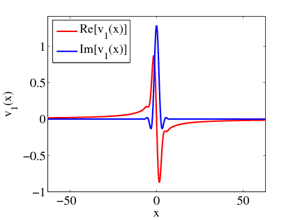
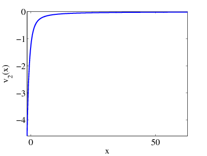
By studying the phases , we see that and are related to and respectively by a parity transformation.
We set and to obtain the front solution of the hyperdiffusion equation:
| (3.37) |
Simplifying and restoring the dimensional units, this is
| (3.38) |
By inspection of the phases , it is clear that the hyperdiffusion equation has no bubble solutions on the whole real line.
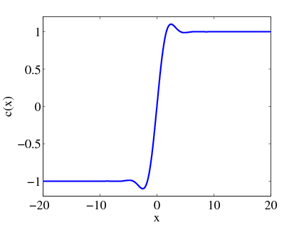
In Fig. 3.10 we present front solution.
Finally we note that the generalized Airy functions give the solution of the nonstationary advection-hyperdiffusion equation
where we have again expressed lengths in terms of the diffusion scale . Time is expressed in terms of the Lyapunov time . By linearity, we may separate the variables, writing . The Airy functions satisfy
| (3.39) |
which is the equation for . Since and do not have the correct far-field behaviour, we are restricted to the dimensional solutions
| (3.40) |
The functions have the asymptotic form , for [94], and therefore have the correct far-field behaviour. Thus, in the absence of segregation, a bubble profile will decay in time owing to the twin processes of advection and hyperdiffusion.
Numerical simulations of the boundary value problem
Armed with this knowledge, we attempt a numerical solution of the boundary-value problem (BVP)
| (3.41) |
where lengths are measured in terms of the transition layer width . The analytic study of the hyperdiffusive limit suggested that seeking a bubble solution may not be sensible, and indeed it is not: solving the time-dependent version of Eq. (3.41) with bubble initial conditions, the concentration profile always decays to a constant. We therefore focus on the frontal boundary conditions.
We solve the BVP (3.41) with frontal boundary conditions in Fig. 3.11. The front steepens with increasing . Physically, this corresponds to a strengthening of local shear in the velocity, which forces the filaments of fluid to become narrower. The numerical solution agrees exactly with the analytical solutions in the limit of large and small . At large , the front width has the hyperdiffusive scaling, indicating a regime dominated by hyperdiffusion, in agreement with the full two-dimensional numerical simulations in Sec. 3.5.
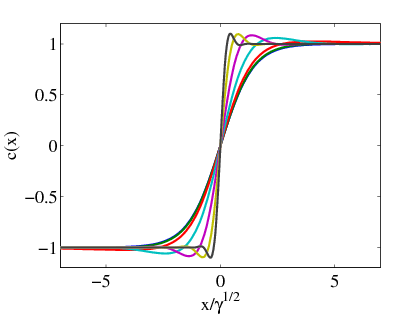
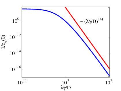
We note that the concentration profile takes values in some places, a consequence of the fact that Eq. (3.25) has no maximum principle, in contrast (say) to the advection-diffusion equation. Again, this result is consistent with the numerical results of Section 3.5, where we find . This superabundance of one binary fluid element is unreasonable on physical grounds, pointing to a shortcoming in the advective CH model. However, we shall see in the next section that the qualitative features of the constant-mobility model and those of the more realistic variable-mobility model are in agreement, suggesting that the simpler model gives an adequate description of advective phase-separation dynamics.
3.7 The variable-mobility case
To gain further insight into the dependence of the bubble size on the Lifshitz-Slyozov and Lyapunov exponents, we study the variable-mobility Cahn–Hilliard equation [95]
| (3.42) |
where as before . By introducing this additional feature, we recover a system that, at least in the case without flow, has a solution confined to the range [8].
We specify the functional form of the mobility as
| (3.43) |
fixing . This modification corresponds to interface-driven coarsening because inside bubbles () the mobility is zero. For other values of we have a mixture of bulk- and interface-driven coarsening. This equation has been investigated by Bray and Emmott [96] for , in an evaporation-condensation picture. They show that the typical bubble size grows as , a result limited to dimensions greater than two. Numerical simulations [5] suggest that this growth law also holds in two dimensions. We couple the modified segregation dynamics to the sine flow.
For , we obtain the growth law for the scale , namely . The growth exponent is close to the value predicted by the LS theory. In addition, we obtain the free energy decay laws again close to the LS value. Thus, as in the constant-mobility case, a description of the problem lengthscales can be given in terms of the bubble energy or in terms of , with identical results.
Because the variable-mobility calculation is computationally slower, we shall perform the numerical experiments with flow at lower resolution. We do not anticipate that this will change the results, because in integrations of the constant-mobility equations at resolution the scaling exponents were unaffected. Switching on the chaotic flow, we observe the steady state, characterized by the fluctuation of the free energy, the wavenumber ,
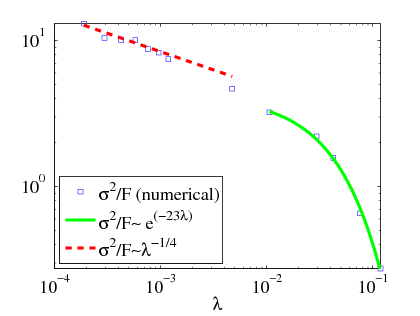
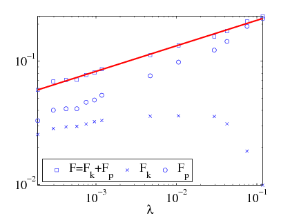
and the variance around mean values. As in the constant-mobility case, the graph of the time-averaged free energy and time-averaged Batchelor scale possess clear scaling laws, while the graph of the mean wavenumber does not. For small , the proxy for bubble radius scales approximately as , suggesting a decay of bubble radius according to the LS exponent. Thus, the analogous result of Section 3.5 is not fortuitous. For large this quantity decays exponentially to zero at a rate (with respect to ) close to that of the constant-mobility system. In each case, the fit of the data is not as good as the constant-mobility case, the computational error being larger here because we have run the simulations at resolution . We present these results in Fig. 3.12.
The results are an exact replica of those for the constant-mobility case. The arrest of bubble growth for small is therefore a genuine phenomenon whose behaviour depends on the LS exponent of the corresponding unstirred dynamics. The mixing at large is identical to that for which the mobility is constant. Thus, while the variable-mobility model is more realistic than its constant-mobility counterpart, their properties with regard to chaotic stirring and eventual mixing are the same.
3.8 Summary
We have shown how, in the presence of an external chaotic stirring, the coarsening dynamics of the Cahn–Hilliard equation are arrested and bubbles form on a particular lengthscale. The system reaches a steady state, characterized by the fluctuation of the free energy , the variance , and the wavenumber around mean values. A measure of the typical bubble size is given by the time average of . For sufficiently large stirring intensities, the bubbles diminish in prominence, to be replaced by filament structures. These are due to the combination of the advection and hyperdiffusion terms in the CH demixing mechanism. In this regime, the concentration tends to homogenize, so that the stirring stabilizes the previously unstable mixed state.
We have explained with a one-dimensional model how this transition arises and how the filament width in the homogeneous regime depends on the Lyapunov exponent of the chaotic flow. This latter investigation exhibits the local superabundance of one of the binary fluid components, which we reject as unreasonable. In the case of no flow this difficulty was overcome by the addition of a variable mobility [8]. However, the quasi-diffusive regime identified in our simulations is robust in the sense that it is present in both the constant- and the more realistic variable-mobility cases. We therefore expect to see this remixing phenomenon in real binary fluids.
Chapter 4 Estimating mixedness in a stirred Cahn–Hilliard fluid
4.1 Overview
In this chapter we study the advective Cahn–Hilliard equation in the passive setting, in the presence of sources and sinks of matter. We focus on the symmetric mixture, which contains equal amounts of each binary fluid component. We have mentioned the often undesirable coarsening tendency of the binary fluid, and the efforts made to suppress it. We therefore introduce a quantitative measure of coarsening suppression by studying the power-mean fluctuation of the concentration about its average value. By fluctuations about the average value, we mean spatial fluctuations around the average spatial concentration (which is zero for a symmetric mixture); we then average these fluctuations over space and time. In effect, we study the time-averaged norm of the concentration. If this quantity is small, the average deviation of the system about the well-mixed state is small, and we therefore use this quantity as a proxy for the level of mixedness of the fluid.
In many applications, the Cahn–Hilliard equation is driven by some external effect, for example, chemically patterned substrates [97], electrically charged media [98], or the subject of this report, stirring. In this chapter, we focus on phase separation in the presence of advection and a source term in the Cahn–Hilliard equation. This source term arises in a number of ways. In [88] it is maintained by thermal diffusion, through the Ludwig–Soret effect [99], in which concentration gradients are induced by imposed temperature gradients. One can also produce concentration gradients by simply injecting matter into the system. The approach we take here is motivated by studies of the advection-diffusion equation [28, 29, 30, 31]. There, the problem is a linear one, and describes miscible liquids, while fluctuations about the mean are measured by the variance or centred second power-mean of the fluid concentration [32, 33]. The variance is reduced by certain stirring mechanisms. By specifying a source term, it is possible to state the maximum amount by which a given flow can reduce the variance, and hence mix the fluid. By quantifying the variance reduction, we can classify flows according to how effective they are at mixing.
4.2 Measures of mixedness
In this section, we introduce the advective Cahn–Hilliard equation with sources and recall some the properties of this equation. We outline the tools and notation we shall use to analyze concentration fluctuations. The results will be valid in any spatial dimension.
We study the advective Cahn–Hilliard equation in the presence of flow, and for prescribed sources and sinks,
| (4.1) |
Here is Cahn–Hilliard diffusion and is the typical thickness of transition zones between phase-separated regions of the binary fluid.
In this chapter we work with a nondimensionalization of Eq. (4.1) that leaves three control parameters in the problem. Therefore, we can unambiguously study limits where control parameters take large or small values. Let be a timescale associated with the velocity , and let be the magnitude of . Let be the magnitude of the source variations and finally, let be a lengthscale in the problem; for example, if the problem is solved in a hypercube with periodic boundary conditions, we take the lengthscale to be the cube length. It is then possible to write down Eq. (4.1) using a nondimensional time and a nondimensional spatial variable ,
and are dimensionless shape functions, , , , and where . As before, the quantity is identified with the ratio , being the ratio of the velocity timescale to the diffusion timescale. Following standard practice, we shall now work with the dimensionless version of the equation, and omit the prime notation. For ease of notation, we shall henceforth take to mean .
We recall the following properties of (4.1) from Ch. 2. These will be useful in what follows.
-
•
If the source is chosen to have spatial mean zero, then the total mass is conserved,
where is the problem domain in dimensions and is its volume. The boundary terms in this equation vanish on choosing no-flux boundary conditions on , or periodic boundary conditions. Here is the outward normal derivative. For simplicity we consider the periodic case, although this is not necessary.
-
•
There is a free-energy functional
(4.2) where is the chemical potential of the system. For a smooth concentration field , the free energy satisfies the evolution equation
and in the absence of sources and stirring decays in time.
To study the spatial fluctuations in concentration, we consider the power means of the quantity ,
| (4.3) |
For a symmetric mixture in which , this is simply
where we have introduced the norm of the concentration, . The quantity is a measure of the magnitude of spatial fluctuations in the concentration about the mean, at a given time. Since we are interested in the ultimate state of the system, we study the long-time average of concentration fluctuations. We therefore focus on the power-mean fluctuations
where is the long-time average
provided the limit exists. We shall repeatedly use the following results for the monotonicity of norms,
| (4.4) |
discussed in Ch. 2.
The Cahn–Hilliard equation and its free energy functional contain high powers of the concentration ( and respectively), and we can therefore estimate for specific -values. In particular, in the following sections, we shall prove the following result in dimensions:
Given a smooth solution to the advective Cahn–Hilliard equation, the long-time average of the free energy exists, and therefore exists, for .
The only constraints we impose on the external forces are that the velocity, its derivatives, and the source term be always and everywhere bounded. We take our result one step further by explicitly evaluating upper and lower bounds for , and this gives a way of quantifying concentration fluctuations in the stirred binary fluid.
4.3 Existence of long-time averages
In this section, we prove a result concerning the existence of the long-time average of the free energy, and of the power means , for .
Given the velocity field , the source , and smooth initial data for the advective Cahn–Hilliard (4.1), the long-time average of the free energy exists, and thus exists, for .
The proof relies on the free-energy evolution equation. Using this law, we find uniform bounds on the finite-time means and , where
Using the monotonicity of norms, the uniform boundedness of , follows, for . The proof proceeds in multiple steps, which we outline below.
Step 1: Analysis of the free-energy evolution equation
Given the conditions on the external forces outlined above, and the results in Ch. 2, there is a unique smooth solution to the advective Cahn–Hilliard equation (4.1), at least for finite times. Thus, we turn to the question of the long-time behaviour of solutions. We exploit the smoothness property of the concentration field in formulating an evolution equation for the free energy. The free energy of the Cahn–Hilliard fluid is
Given the smooth, finite-time solution , we differentiate the functional with respect to time and obtain the relation
using the no-flux or periodic boundary conditions. By averaging this equation over finite times, we obtain the identity
| (4.5) |
We single out the quantity for study. Owing to the nonnegativity of , we have the inequality . Therefore, we need only consider two possible cases: , and . We shall show that is not possible, and in doing so, we shall produce a uniform (-independent) upper bound on .
Let us assume for contradiction that . Then, given any in the range , there is a time such that , for all times . Thus, for times , the time average is strictly positive. Henceforth, the inequality is assumed. Using , Eq. (4.5) becomes
| (4.6) |
As in Sec. 2.6, we use the following string of relations,
where we have used the antisymmetry of the operator to deduce that
for any function . The quadratic form satisfies
which gives rise to the inequality
| (4.7) |
The matrix is the stretching tensor [100], the appearance of which highlights the importance of shear and stretching in the development of the morphology of the concentration field [20].
For each time , we split the chemical potential into a part with mean zero, and a mean component: , where . Then, for any function with spatial mean zero, we have the relation . Using this projection relation, Eq. (4.6) becomes
Owing to the positivity of , we have the inequality
| (4.8) |
Finally, we employ the Poincaré inequality for mean-zero functions on a periodic domain :
| (4.9) |
Combining Eqs. (4.7), (4.8), and (4.9) gives the following inequality:
| (4.10) |
where . There are no angle brackets around the source term because is independent of time.
Step 2: Obtaining a bound on
Step 3: An upper bound on
We have the free energy
Hence,
Time averaging both sides and using the monotonicity of norms (4.4), we obtain the result
Using the bound for in (4.12), this becomes
We therefore have a -independent equation for the upper bound on ,
| (4.13) |
where solves the polynomial
| (4.14) |
The highest power of on the left-hand side is , while the highest power of on the right-hand side is . Thus, this equation always has a positive solution, and moreover this positive solution is unique.
We obtain the following chain of uniform (-independent) bounds. Each bound follows from the previous bounds in the chain, and the first bound follows from Eq. (4.13).
-
•
is uniformly bounded,
-
•
is uniformly bounded,
-
•
is uniformly bounded,
-
•
is uniformly bounded,
-
•
is uniformly bounded,
(4.15)
for all . Owing to the uniformity of these bounds, they hold in the limit . The result implies the existence of a uniform bound for , almost everywhere. Given the differentiability of , this implies that is everywhere uniformly bounded, and thus, , which is a contradiction. Therefore, the only possibility for is that it be zero. It is straightforward to verify that by taking , and making slight alterations in Steps 1–3, the bounds in Eq. (4.15) still hold.
Let us examine the significance of our result. We have shown that for sufficiently regular flows and source terms (specifically, , for all , and ), there is an a priori bound on the free energy . We have shown that the system always reaches a steady state, in the sense that . We have also found an upper bound for the measure of concentration fluctuations, as the unique positive root of the polynomial equation Eq. (4.14). This bound depends only on the source amplitude, the diffusion constant, and the maximum stretching . Using the monotonicity of norms, this number serves also as an upper bound on for . Let us comment briefly on the volume term in the equation . Since this upper bound includes many situations, it must take into account the case where both the velocity and the source vanish. Then as , and by definition, , which is in agreement with Eq. (4.14). These results enhance the existence theory obtained in Sec. 2.6, and give information about the long-time behaviour of solutions.
As mentioned in Ch. 1, it is desirable in many applications to suppress concentration fluctuations, since this leads to a homogeneous mixture. In this report, we use advection as a suppression mechanism, and we would therefore like to know the maximum suppression achievable for a given flow. This inspires us to seek lower bounds on , in addition to the upper bounds found in this section.
4.4 Lower bounds on the concentration fluctuations
In this section we discuss the significance of the lower bound on the measure of concentration fluctuations. Due to the powers of the concentration that appear in the Cahn–Hilliard equation, it is possible to obtain an explicit lower bound for , which we then use to discuss stirring as a mechanism to suppress concentration fluctuations. Using Hölder’s inequality, a flow that suppresses concentration fluctuations in the sense will also suppress them in the sense, for , and thus our discussion of the suppression of concentration fluctuations by stirring is valid in this broader sense.
As discussed in Sec. 5.2, a suitable measure of concentration fluctuations for a symmetric mixture is
where is the concentration of the binary mixture and is its norm. For , this gives the usual variance, used in the theory of miscible fluid mixing [29, 28, 30, 31]. In that case, the choice is a natural one suggested by the linearity of the advection-diffusion equation. In the following analysis of the advective Cahn–Hilliard equation, it is possible to find an explicit lower bound for and we therefore use this quantity to study the suppression of concentration fluctuations due to the imposed velocity field. Given this formula, we can compare the suppression achieved by a given flow with the ideal level of suppression, and decide on the best strategy to homogenize the binary fluid.
To estimate , we take Eq. (2.2), multiply it by an arbitrary, spatially-varying test function , and then integrate over space and time, which yields
| (4.16) |
where is the linear operator . Using the constraint equation (4.16), the monotonicity of norms, and the Cauchy–Schwarz inequality, we obtain the following string of inequalities,
which gives the relation
We study the denominator
where this bound follows from the triangle and Hölder inequalities. Thus we have the result
or
Using the monotonicity of norms (4.4), we recast this inequality as one involving only a single power-mean,
Therefore, we have the following inequality for ,
where
Thus, we obtain a lower bound for the measure of concentration fluctuations,
| (4.17) |
The cubic equation satisfied by has a unique positive root.
To probe the asymptotic forms of (4.17), we rewrite the forcing terms and as an amplitude, multiplied by a dimensionless shape function. Thus,
| , | ||||
| , |
Then for a fixed value of and , and (large stirring), we have , and the lower bound takes the form
On the other hand, for fixed and , and (large diffusion), the lower bound takes the form
It is possible to obtain similar asymptotic expressions for , by minimizing a constrained functional of the concentration. Apart from a volume factor, the asymptotic form of agrees exactly with the asymptotic form of just obtained. The functional to be minimized is
where is a test function and is the Lagrange multiplier for the constraint. This approach has been taken in [30] for the advection-diffusion equation. Setting gives
| (4.18) |
Evaluation of shows that Eq. (4.18) produces a minimum of . Given the expression , the minimum Eq. (4.18) is at large . Substitution of this expression into the constraint
gives , and hence
For fixed and and large , a similar calculation gives
These expressions show that, apart from a volume factor, the lower bounds on the and measures of concentration fluctuations are identical in the physically interesting limits of high stirring strength, or high diffusion. In particular, the expression
indicates that if a flow can be found that saturates the lower bound , the suppression of concentration fluctuations can be enhanced by a factor of at large stirring amplitudes. Such a flow would then be an efficient way of mixing the binary fluid.
4.5 Scaling laws for
In this section we investigate the dependence of the measure of concentration fluctuations on the parameters of the problem, namely the stirring velocity , the source , and the diffusion constant . For simplicity, we shall restrict our interest to a certain class of flows, which enables us to compute long-time averages explicitly.
The lower bound for the measure of concentration fluctuations is the unique positive root of the polynomial
| (4.19) |
where is a test function and
We specialize to velocity fields whose time average has the following properties,
| (4.20) |
The flow is defined on the -torus . A statistically homogeneous and isotropic turbulent velocity field automatically satisfies the relations (4.20), although it is not necessary for to be of this type. The source we consider is monochromatic (that is, it contains contains a single spatial scale) and varies in a single direction,
| (4.21) |
Our choice of velocity field makes the evaluation of particularly easy; it is
In studies of the advection-diffusion equation [30], it is possible to find an explicit test function that sharpens the lower bound on . The procedure for doing this depends on the linearity of the equation. Here, this is not possible, and for simplicity we set . This choice of certainly gives a lower bound for the measure of concentration fluctuations, with the added advantage of enabling explicit computations. Having specified the coefficients of the polynomial in Eq. (4.19) completely, we extract the positive root of this equation, and find the lower bound , as a function of . The results of this procedure are shown in Fig. 4.1.
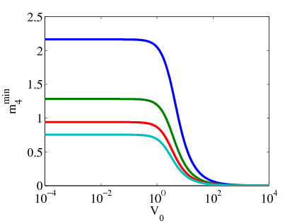
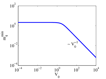
Let us examine briefly the scaling of the upper bound with the problem parameters. The upper bound satisfies the polynomial equation
| (4.22) |
which depends only on the diffusion , the source amplitude , and the maximum stretching . For large , the flow-dependence of the upper bound is . This dependence is verified by obtaining the positive root of Eq. (4.22), which is as a function of . The results are shown in Fig. 4.2.
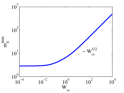
Mixedness at small scales
In the same manner, we find a lower bound for the quantity . A similar gradient norm has arisen in the problem of quantifying mixedness at small scales in the theory of miscible fluids [30]. Using the constraint equation (4.16) again, we find
where . We study the denominator
Using the Gagliardo–Nirenberg–Sobolev inequality on the periodic domain , we obtain
Thus, the denominator is bounded above by
We therefore have the inequality
and hence
| (4.24) |
where
For a velocity field with the time-average relation , this is
This concludes our investigation into lower bounds on the level of mixedness achievable in a stirred, phase-separating fluid. We note briefly that for any nonzero source, the lower bound is nonzero, meaning that no matter how hard one stirs, there will always be some inhomogeneity in the fluid, and this is in fact true for any flow. However, the quantity tells us how much homogeneity we can achieve and is therefore a yardstick for stirring protocols. We use this yardstick to test model flows in the next section.
4.6 Numerical simulations
In this section we solve Eq. (2.2) numerically for two flows, and verify the bounds obtained in Secs. 4.3–4.5. We use the sinusoidal source term in Eq. (4.21) with periodic boundary conditions, and the source scale therefore takes the form , where is the box size and is an integer. We specialize to two dimensions and study two standard flows that are used in the analysis of mixing: the random-phase sine flow of Sec. 3.3, and the constant flow [31].
Random-phase sine flow
The random-phase sine flow is the time-dependent two-dimensional flow
| (4.25) |
where and are phases that are randomized once during each flow period , and where the integer labels the period. The flow is defined on the two-dimensional torus . The time average of this velocity field has the properties listed in Eq. (4.20). We solve Eq. (2.2) with the flow in Eq. (4.25) as in Sec. 3.3. Recall that we used the lattice method for advection [24, 27], which was effective only when the spread of matter due to diffusion is much slower than the spread due to advection, that is, . Thus, as before, we therefore set , while we set . A numerical experiment with shows that gives rise to a morphology that is qualitatively different from the sourceless morphology, and we therefore work with this source amplitude. Finally, following standard practice [16, 20], we choose , the gridsize.
Using this nondimensionalization, and the identity for the sine flow, we recall the large-stirring forms of . For , the lower bound has the form
| (4.26) |
with the power-law relationship , while for the upper bound has the form
| (4.27) |
These scaling results are identical to those for the advection-diffusion problem [28].
Before studying the case with flow, we integrate Eq. (2.2) without flow, to verify the effect of the source.
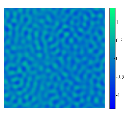
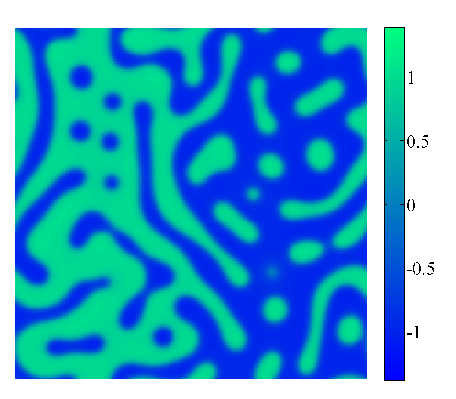
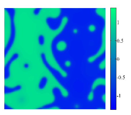
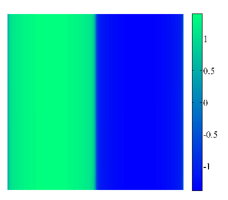
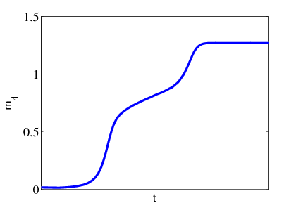
For a sufficiently large source amplitude, the concentration phase separates and forms domains rich in either binary fluid component. These domains are aligned with variations in the source. A steady state is reached and attains a constant value, as seen in Fig. 4.3. On the other hand, for small source amplitudes, we have verified that that the domains do not align with the source, and their growth does not saturate. We do not consider this case here, since we are interested in sources that qualitatively alter the phase separation. These different regimes are discussed in [88].
We consider the case with flow by varying , and find results that are similar to those found in Sec. 3.5, for the same stirring mechanism without sources. For all values of , the concentration reaches a steady state, in which , effectively the pre-averaged form of , fluctuates around a constant value. For small values of , the domain growth is arrested due to a balance between the advection and phase-separation terms in the equation, while for moderate values of , the domains are broken up and a mixed state is obtained. At large values of , the measure of concentration fluctuations saturates: further increases in do not produce further decreases in . At these large values of , the source structure is visible in snapshots of the concentration, as evidenced by Fig. 4.4.
We investigate the dependence of concentration fluctuations on the stirring strength , and show the results in Fig. 4.5. The theoretical upper and lower bounds on depend on and are obtained as as roots of Eqs. (4.19) and (4.22). In the limit of large , these bounds have power-law behaviour, with and , as demonstrated by Eqs. (4.26) and (4.27). The numerical values of are indeed bounded by these limiting values, although the -dependence is not a power law. Instead, the function
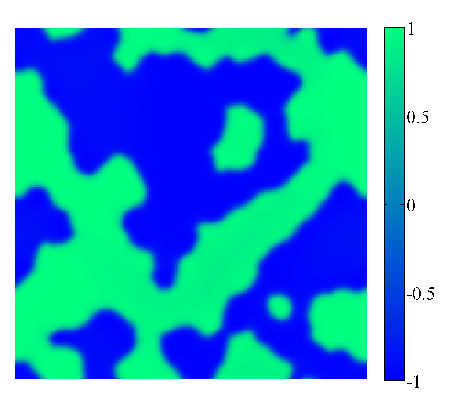
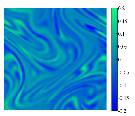
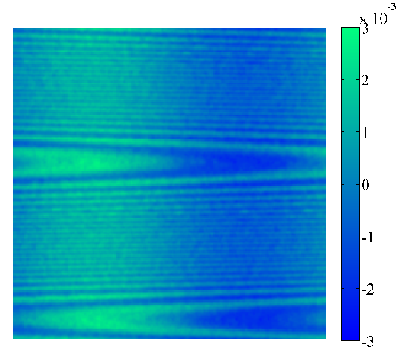
is a nonincreasing function, with a sharp drop occurring in a small range of -values. Thus, the fluid becomes more homogeneous with increasing . We discuss the effect of stirring on the inhomogeneity of the fluid by introducing the notion of mixing efficacy.
We measure the ability of a given stirring protocol to suppress concentration fluctuations by the mixing efficacy. Similar ideas are often applied to the advection-diffusion equation [28, 29, 30, 31]. We define the dimensionless mixing efficacy
For a given flow, the number quantifies the flow’s ability to suppress concentration fluctuations. In a well-mixed flow, the local deviation of away from the mean will be small; a small -value is a signature of a well-mixed flow. We are therefore justified in calling the mixing efficacy. We obtain some control over the mixing efficacy from the inequalities of Secs. 4.2 and 4.4. Based on these inequalities, the mixing efficacy is bounded above and below,
We have plotted the upper and lower bounds on the mixing efficacy for the case of monochromatic sources in Fig. 4.5 (b). The maximum efficacy
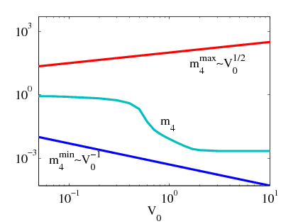
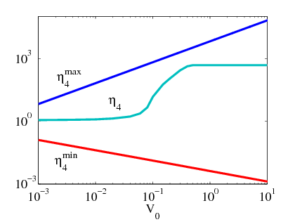
always exceeds unity in this case, which implies the possibility of finding stirring protocols that homogenize the fluid. On the other hand, the minimum efficacy is less than unity, which indicates the possibility of finding stirring protocols that actually enhance concentration fluctuations, and this enhancement depends weakly on the maximum stretching . This latter case is not surprising, given that a uniform shear flow causes the domains of the Cahn–Hilliard fluid to align, rather than to break up. The sine-flow efficacy is a nondecreasing function of the stirring parameter . At small values of , small increases in the vigour of stirring lead to small increases in the mixing efficacy. There is a window of intermediate -values for which the mixing efficacy increases sharply with increasing . At higher values of , the efficiency saturates, so that further increases in the vigour of stirring have no effect on concentration fluctuations. In the saturated case, the concentration field mirrors the structure of the source function, as in Fig. 4.4 (c).
Constant flow
We study the flow , where is a constant. We choose a nondimensionalization that is set by the diffusion time , and obtain the following parametric version of Eq. (2.2),
| (4.28) |
where , , and . We immediately drop the primes from Eq. (4.28). We fix and and vary the flow strength . As in the case of no flow, we choose such that the morpohology is qualitatively different from the sourceless one; in the units used here, we set . This flow does not satisfy the time-correlation relations (4.20), although the maximum stretching has the simple form . The
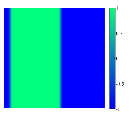
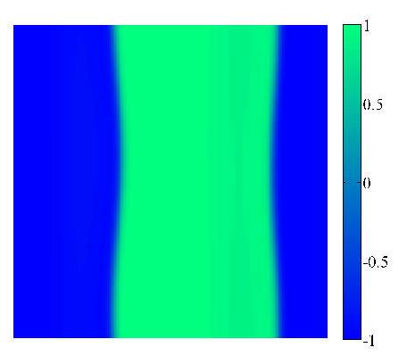
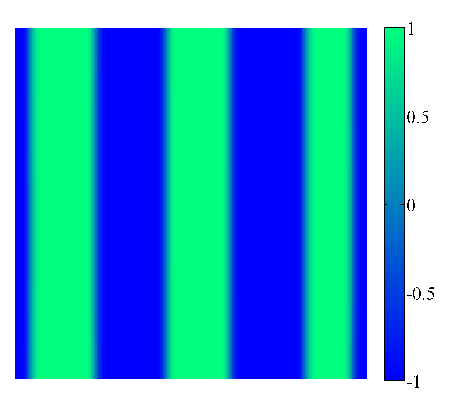
upper bound obtained in Eq. (4.14) is therefore independent of the flow strength.
We solve Eq. (4.28) numerically for various values of and present the results in Fig. 4.6. For small , the morphology of the concentration field is similar to the flowless case seen in Fig. 4.3 (d), except now the domains are uniformly advected in a direction perpendicular to the source variation. The small- case is shown in Fig. 4.6 (a). As increases, the domain boundaries are distorted due to the advection, while for large , the advection is sufficiently strong to precipitate the formation of narrower lamellae, although the domain structure persists.
The measure of mixedness extracted from the numerical simulations is almost constant across the range of stirring parameters , and resides in the range defined by the bounds in Sec. 4.4. For , is slightly smaller than its value at , due to the presence of more interfaces. This difference is small however, and increasing does little to mix the fluid. This is not surprising, given that local shears are necessary to break up domain structures [20], and that such shears are absent from constant flows. What this example shows however, is the difference between a miscible mixture, and a phase-separating mixture. For a diffusive mixture with the sinusoidal source we have studied, the constant flow discussed here is optimal for mixing [31]; for a phase-separating mixture, the constant flow badly fails to homogenize the mixture.
4.7 Summary
We have introduced the advective Cahn–Hilliard equation with a mean-zero driving term as a way of describing a stirred, phase-separating fluid, in the presence of sources and sinks. By specializing to symmetric mixtures, we have studied a more tractable problem, although one with many applications.
Our goal was to investigate stirring protocols numerically and analytically, and to determine the best way to break up the domains in the Cahn–Hilliard fluid and achieve homogenization. To this end, we introduced the measure of concentration fluctuations. Since in a well-mixed fluid, the concentration exhibits small spatial fluctuations about the mean, with better mixing leading to smaller fluctuations, we used as a measure of mixedness or homogeneity. We proved the existence of for long times, for , and obtained a priori upper and lower bounds on , as an explicit function of the imposed flow , and the source .
We compared the level homogeneity achieved by the random-phase sine flow and the constant flow with the lower bound, and found that the sine flow is effective at homogenizing the binary fluid, while the constant flow fails in this task. This is not surprising, since it is known that differential shears are needed to break up binary fluid domains, although it is radically different from the advection-diffusion case, where the constant flow was the optimal mixer. The question of whether or not a flow is a good mixer in this context was discussed using the mixing efficacy, defined in Sec. 4.6. Given such a definition, it is possible to compare stirring protocols and find the optimal protocol for mixing a binary fluid. Our upper bound on the efficacy provides a meaningful notion of this optimality. This result may be useful in applications where the homogenization of a binary fluid is desirable, since we have set a lower limit on precisely how much homogeneity can be achieved.
Chapter 5 Nonlinear dynamics of phase separation in ultra-thin films: Analysis
5.1 Overview
In this chapter we recall the Navier–Stokes Cahn–Hilliard (NSCH) equations derived in Sec. 2.3, shifting focus from the passive tracer, to the active one. We study these equations in the incompressible limit. We shall specialize to thin films, in which the binary liquid forms a thin layer on a substrate. Then, if the vertical gradients are small compared to horizontal ones, a long-wavelength version of the NSCH equations can be obtained, representing a much simplified problem. We present the derivation of these long-wavelength or thin-film Stokes Cahn–Hilliard equations. We analyze these equations and obtain results concerning the existence, regularity, and uniqueness of solutions.
5.2 The thin-film Stokes Cahn–Hilliard equations
In this section we recall the incompressible Navier–Stokes Cahn–Hilliard equations from Sec. 2.3 and discuss the passage from these equations to the long-wavelength approximation in two dimensions. We enumerate the scaling rules necessary to obtain the simplified equations. Finally, we arrive at a set of equations that describe phase separation in a thin film acted on by arbitrary body forces.
The incompressible NSCH equations derived in Sec. 2.3 describe the coupled effects of phase separation and flow in a density-matched binary fluid. If is the fluid velocity and is the concentration of the mixture, where indicates total segregation, then these fields evolve in the following way,
| (5.1a) | |||
| (5.1b) | |||
| (5.1c) | |||
where
| (5.2) |
is the stress tensor, is the fluid pressure, is the body potential and is the constant mixture density. The constant is the kinematic viscosity, , where is the viscosity. Additionally, is a constant with units of , is a constant that gives the typical width of interdomain transitions, and a diffusion coefficient with dimensions .
If the system has a free surface in the vertical or -direction and has infinite or periodic boundary conditions (BCs) in the lateral or -direction, then the vertical BCs we impose are
| (5.3a) | |||
| while on the free surface they are | |||
| (5.3b) | |||
| (5.3c) | |||
| (5.3d) | |||
where is the unit normal to the surface, , is the unit vector tangent to the surface, is the surface coordinate, is the surface tension and is the mean curvature,
This choice of BCs guarantees the conservation of the total mass and volume, respectively
| (5.4) |
Here represents the time-varying domain of integration, whose time dependence is due to the variable nature of the free surface height. Note that in view of the concentration BC (5.3d), the stress BC (5.3b) does not contain or its derivatives.
These equations admit a great simplification if the fluid forms a thin layer of mean thickness , for then the scale of lateral variations is large compared with the scale of vertical variations . This is shown in Fig. 5.1. Specifically, the parameter is small, and after nondimensionalization of Eq. (5.1), we expand its solution in terms of this parameter, keeping only the lowest-order terms. For a review of this method and its applications, see [50]. For simplicity, we work in two dimensions, but the generalization to three dimensions is easily effected.
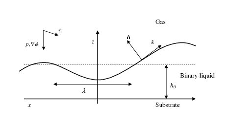
In terms of the small parameter , the equations nondimensionalize as follows. The diffusion timescale is and we choose this to be the unit of time. Then the unit of horizontal velocity is so that , where variables in upper case denote dimensionless quantities. Similarly the vertical velocity is . For the equations of motion to be half-Poiseuille at (in the absence of the backreaction) we choose and . Using these scaling rules, the dimensionless momentum equations are
| (5.5) |
| (5.6) |
where
| (5.7) |
The choice of ordering for the Reynolds number allows us to recover half-Poiseuille flow at . We delay choosing the ordering of the dimensionless group until we have examined the concentration equation, which in nondimensional form is
| (5.8) |
where . By switching off the backreaction in the momentum equations (corresponding to ), we find the trivial solution to the momentum equations, , . The concentration boundary conditions are then on which forces so that the Cahn–Hilliard equation is simply
To make the lubrication approximation consistent, we take
| (5.9) |
We now carry out a long-wavelength approximation to Eq. (5.8), writing , , . We examine the boundary conditions on first. They are on ; on these conditions are simply , while on the surface derivatives are determined by the relations
Thus, the BCs on are simply on , which forces . Similarly, we find , and
In the same manner, we derive the results . Using these facts, equation (5.8) becomes
We now integrate this equation from to and use the boundary conditions
After rearrangement, the concentration equation becomes
where
is the vertically-averaged velocity. Introducing
the thin-film Cahn–Hilliard equation becomes
| (5.10) |
We are now able to perform the long-wavelength approximation to Eqs. (5.5) and (5.6). At lowest order, Eq. (5.6) is
which is simply , and hence
Here
| (5.11) |
is the dimensionless measure of the backreaction strength. Thus, Eq. (5.5) becomes
and using this is
| (5.12) |
At lowest order, the BC (5.3b) becomes
| (5.13) |
where is the dimensionless, spatially-varying surface tension. Combining Eqs. (5.12) and (5.13) yields the relation
Making use of the BC on and integrating again, we obtain the result
| (5.14) |
The vertically-averaged velocity is therefore
Using the standard Laplace–Young free-surface boundary condition, this becomes
where
| (5.15) |
Finally, by integrating the continuity equation in the -direction, we obtain, in a standard way, an equation for free-surface variations,
Let us assemble our results, restoring the lower-case fonts and omitting ornamentation over the nondimensional quantities,
| (5.16a) | |||
| (5.16b) | |||
| where | |||
| (5.16c) | |||
| (5.16d) | |||
and where we have the following nondimensional constants,
These are the thin-film Stokes Cahn–Hilliard (SCH) equations. The integral quantities and defined in Eq. (5.4) are manifestly conserved, while the free surface and concentration are coupled.
We note that the relation is the condition that the mean thickness of the film be much smaller than the transition layer thickness. In experiments involving the smallest film thicknesses attainable ( m) [101], this condition is automatically satisfied. The condition is also realized in ordinary thin films when external effects such as the air-fluid and fluid-substrate interactions do not prefer one binary fluid component or another. In this case, the vertical extent of the domains becomes comparable to the film thickness at late times, the thin film behaves in a quasi two-dimensional way, and the model equations are applicable.
The choice of potential determines the behaviour of solutions. If interactions between the fluid and the substrate and air interfaces are important, the potential should take account of the Van der Waals forces present. A simple model potential is thus
where is the dimensionless Hamakar constant and typically [50]. Here can be positive or negative, with positivity indicating a net attraction between the fluid and the substrate and negativity indicating a net repulsion. This choice of potential can also have a regularizing effect, preventing a singularity or rupture from occurring in Eq. (1.1c).
For (repulsive Van der Waals interaction), the system of equations (1.1c) has a Lyapunov functional , where
and where defines the lateral extent of the system. In this chapter we take to be a periodic domain, which fixes the boundary conditions, although other choices of boundary conditions are possible. By differentiating these expressions with respect to time, we obtain the relation
| (5.17) |
which is nonpositive for nonnegative . This fact holds the key to the analytic results obtained in the next section.
5.3 Existence and regularity of solutions
In this section we prove that solutions to the model equations do indeed exist. We focus on the one-dimensional equation set
| (5.18) |
where
The application we have in mind involves a periodic domain . We shall prove our result for smooth initial conditions,
| (5.19) |
We shall prove that the solutions to this equation pair exist in the strong sense; however, we shall need the following definition of weak solutions:
A pair is a weak solution of Eq. (5.18) if the following integral relations hold,
(5.20) where is any time, and and are arbitrary differentiable test functions that are periodic on and vanish at and .
We address the following statement,
Given the initial data in Eq. (5.19), the equations (5.18) possess a unique strong solution endowed with the following regularity properties:
Recall that the function resides in the class if
The proof is given in the following steps.
5.3.1 Regularization of the problem
We introduce regularized functions and such that
For now we do not specify , although we mention that a suitable choice of will cure the degeneracy of the fourth-order term in the height equation. On the other hand, we require that the function have the following properties:
-
•
, for ,
-
•
, for ,
-
•
,
-
•
has as many derivatives as necessary.
One way of obtaining such a function is to define
| (5.21) |
which is in the variable , and has Lipschitz third derivative; inspection of Eq. (5.18) shows that this degree of smoothness is sufficient to regularize the equations. A sketch of this regularization is shown in Fig. 5.2.
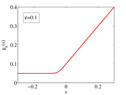
The regularized PDEs we study are thus
| (5.22) |
where
The -equation can also be written as
5.3.2 The Galerkin approximation
We choose a complete orthonormal basis on the interval , with periodic boundary conditions. Let us denote the basis by . We consider the finite-dimensional vector space . For convenience, let us take the ’s to be the eigenfunctions of the Laplacian on with periodic boundary conditions, with corresponding eigenvalues . Moreover, let be the constant eigenfunction. We construct approximate solutions to the PDEs (5.22) as finite sums,
If the (smooth) initial data are given as
then the initial data for the Galerkin approximation are
and the initial data of the Galerkin approximation converge strongly in the norm to the initial data of the unapproximated problem. Thus, there is a such that , everywhere in , for all . Henceforth we work with Galerkin approximations with .
Substitution of into a weak form of the -equation yields
| (5.23) |
where
is the flux for the regularized -equation, and in this chapter, denotes the pairing . This is recast as
where the function depends on
and is locally Lipschitz in its variables. This Lipschitz property arises from the fact that the regularized flux, evaluated at the Galerkin approximation, is a composition of Lipschitz continuous functions, and therefore, is itself Lipschitz continuous.
Similarly, substitution of into the weak form of the -equation yields
| (5.24) |
where
is the flux for the regularized -equation. Rearranging gives
and the left-hand side can be recast in matrix form as , where
which is manifestly symmetric. It is positive definite because given a nonzero vector , we have the relation
which follows from the positivity of the regularized function . We therefore have the following equation for ,
| (5.25) |
Inspecting the expression for , , and , we see that and appear in a (locally) Lipschitz-continuous way in the expression , while owing to the imposed smoothness of , the variables , and appear in a Lipschitz-continuous way in the quantity
The vector can be replaced by the function and thus we obtain a relation
in place of Eq. (5.25), where is Lipschitz. We therefore have a system of Lipschitz-continuous equations
and thus local existence theory guarantees a solution for the ’s and ’s for all times in a finite interval . This solution is, moreover, unique and continuous.
5.3.3 A priori bounds on the Galerkin approximation
We identify the free energy
where . Since the Galerkin approximation satisfies the weak form of the PDEs given in Eqs. (5.23) and (5.24), it is possible to obtain the following free-energy decay law,
| (5.26) |
where . Now given the time continuity of in , and the initial condition (since ), there is a time , such that , and such that for all and all . Therefore, for , and hence
for . Consequently, we obtain the bound , where , and where depends only on the initial conditions. We have Poincaré’s inequality for ,
Now . Inspection of Eq. (5.23) shows that . Thus,
Using the following inequality from Sec. 2.4,
we obtain the bound
and hence . Additionally, the following properties hold:
-
•
The function is Hölder continuous in space, with exponent ,
-
•
,
where these results hold in , and where the constants , , , and are independent of , , , and , and in fact depend only on the functions and .
In order to continue the estimates to the whole interval , we need to prove that almost everywhere (a.e.). If this is true, there is a new interval , , on which a.e., and we can then provide a priori bounds on and on the interval . It is then possible to show that a.e. and thus, by iteration, we extend the proof to the whole interval , and find that a.e. on .
We have the bound
| (5.27) |
where depends only on the initial conditions, and where . We now specify , in more detail. This function satisfies the condition
We take to be as defined previously, while can be regularized as , which is Lipschitz continuous. By defining
we obtain a function that is positive for all , and
Using the boundedness of , and the time continuity of , we employ the Dominated Convergence Theorem,
Similarly, since the constant in the inequality , depends only on the initial data, we extend this last inequality to , and thus is Hölder continuous in space.
In the worst-case scenario, the time is the first time at which touches down to zero, and and we therefore assume for contradiction that , and that elsewhere. Then by the Hölder continuity, for any we have the bound , and thus
Hence,
Thus, the integral can be made arbitrarily large, which contradicts the -independent bound for this quantity, obtained in Eq. (5.27). We therefore have the strong condition that set on which is empty. Iterating the argument, we have the following important result:
The set on which is empty, for .
Using the same argument, we have an estimate on the minimum value of ,
namely,
for all small positive . Thus,
| (5.28) |
a result that depends only on the initial data and . Now, using Eq. (5.28) and the boundedness result
where depends only on the initial data, we obtain a priori bounds on ,
It is also possible to derive a bound on . We have the relation
which gives the inequality Using the Hölder relation , we obtain a quadratic inequality in ,
with solution
as required. From the boundedness of and follows the relation , a result that depends only on the initial conditions. Let us recapitulate these results:
-
•
, is uniformly bounded;
-
•
is uniformly bounded;
-
•
The function is Hölder continuous in space, with exponent ;
-
•
The function is nonzero everywhere and never decreases below a certain value , independent of , , and .
-
•
is uniformly bounded;
-
•
is uniformly bounded;
-
•
The function is Hölder continuous in space, with exponent ,
where these results are independent of , and , and hold for .
5.3.4 Equicontinuity of the Galerkin approximation; convergence of Galerkin approximation
Using Eq. (5.26), we obtain the bound
a bound that is independent of , , and . Since the quantity is bounded above by a constant independent of , , and , we have the following string of inequalities,
and thus
where is independent of , , and . Similarly,
and
where and are independent of , , and . By rewriting the evolution equations as
where , we see that there are uniform bounds for and , which depend only on the initial data and . We mention the following result due Bernis and Friedman [53].
[Bernis and Friedman, 1990] Let be a sequence of functions that weakly satisfy the equation
If is Hölder continuous (exponent ), and if the fluxes satisfy
where is a number independent of the index and the time , then there is a constant , independent of and , such that
for all and in .
We now observe that the fluxes , and satisfy the conditions of this theorem, and thus
The functions and are Hölder continuous (exponent ), for .
We therefore have a uniformly bounded and equicontinuous family of functions . We also have a recipe for constructing a uniformly bounded and equicontinuous approximate solution , in a small interval . The recipe can be iterated step-by-step, and we obtain a uniformly bounded and equicontinuous family of approximate solutions , on , for an arbitrary time . Then, using the Arzelà–Ascoli theorem, we obtain the following convergence result:
There is a subsequence of the family that converges uniformly to a limit , in .
In contrast to Ch. 2, this convergence result is uniform and true everywhere in (uniform strong convergence). We prove several facts about the pair .
Let be the limit of the family of functions constructed in Steps (5.3.1)–(5.3.4). Then the following properties hold for this limit:
- 1.
The functions and are uniformly Hölder continuous in space (exponent ), and uniformly Hölder continuous in time (exponent );
- 2.
The initial condition holds;
- 3.
satisfy the boundary conditions of the original problem (periodic boundary conditions);
- 4.
The derivatives , , , , and are continuous in the set ;
- 5.
The function pair satisfy the following weak form of the PDEs,
where and are suitable test functions.
The statements (1), (2), and (3) are obvious. Now, any pair satisfies the equation set
and from the boundedness of the fluxes and in , it follows that
for a subsequence. Using the regularity theory for uniformly parabolic equations and the uniform Hölder continuity of the ’s, it follows that
The derivatives , , , and are uniformly convergent in any compact subset of .
Thus,
on , and therefore Claims (4) and (5) follow.
5.3.5 Convergence of regularized problem, as
The result in Step (5.3.4) produced a solution to the regularized problem. Due to the result
| (5.29) |
independent of , the argument of Step (5.3.4) can be recycled to produce a solution to the unregularized problem. This solution is constructed as a limit , and the results of the theorem in Step (5.3.4) apply again to . The result (5.29) applies to constructed as , and thus all the derivatives , , , , and are continuous on the whole space and therefore, the weak solution is in fact a strong one.
5.3.6 Regularity properties of the solution
Using a bootstrap argument, we show that the solution belongs to the regularity classes and . From Step (5.3.3) it follows immediately that
with time-independent bounds. Thus, using Poincaré’s inequality, it follows that and, moreover,
From Step (5.3.4), it follows that and belong to the regularity class , and hence , . The functions , , and take the form
and
respectively. The following results will help us in our demonstration,
-
•
We shall use the boundedness of ,
and the boundedness of , .
-
•
Since , it follows that , by Poincaré’s inequality.
-
•
From this it follows that is in the class .
-
•
We have the inequality
and thus .
-
•
Similarly, since , we have the result .
Now inspection of shows that is in , from which follows the result . By repeating the same argument, we find that . We also have the result that is almost always bounded. To show that , we take the evolution equation for , multiply it by , and integrate, obtaining
where . The time integral of the first term on the left-hand side of this equation is obviously bounded in time. Let us examine the time integral of the second term,
The third term on the left-hand side is despatched with in a similar way, so that . We have now shown that
Using this result, together with the previous facts gathered together in this section, it is readily shown that
And finally, using this result, it follows that
For example,
This bound, together with the result , implies that
Similarly,
Hence , and by symmetry, . Since
is in , it follows that is in this class too. A similar argument holds for . Thus, the solution belongs to the following regularity class:
| (5.30) |
Extra regularity is obtained by writing the equation pair as
where
for any , and where and belong to the class . By multiplying the height and concentration equations by and respectively, and by integrating over space and time, it is readily shown that
and hence
from which follows the regularity result
| (5.31) |
5.3.7 Uniqueness of solutions
Let us consider two solution pairs and and form the difference . Given the initial conditions , we show that for all time, that is, that the solution we have constructed is unique. We observe that that the equation for the difference can be written in the form
| (5.32) |
where , and where . Thus, using the semigroup theory of Sec. 2.5, we find that Eq. (5.32) has a unique solution. Since satisfies Eq. (5.32), and since , it follows that for all times .
It is now possible to formulate an equation for the difference by subtracting the evolution equations of and from one another, mindful that . We multiply the resulting equation by and integrate over space, obtaining the result
Using the lower bound on and Young’s first inequality, this equation is transformed into an inequality,
where , , and are arbitrary positive constants. By choosing , the inequality simplifies,
which in turn reduces to
where is another positive constant. We integrate over the time interval , and use the fact that to obtain the string of inequalities
The Poincaré inequality can be combined with the one-dimensional differential inequalities discussed in Ch. 2 to yield the relation , where is some mean-zero function and is an -independent constant. We therefore arrive at the inequality
Using the results of Sec. 5.3.6, it is readily shown that , and that the functions and belong to the class . By choosing sufficiently small, it is possible to impose the inequality
which in turn forces , and hence the solution is unique.
5.4 Summary
In this chapter we have switched focus from the passive to the active tracer. The jump in complexity is significant, and involves the Navier–Stokes Cahn–Hilliard equations. We focus on the case where the active system forms a thin layer on a substrate, and obtain simplified thin-film Stokes Cahn–Hilliard equations that are valid when the system’s vertical gradients are small compared to the those in the lateral directions. We analyze these equations in one lateral dimension, using the tools developed in Ch. 2, and prove existence, regularity, and uniqueness results for the equations. While this analysis yields many precise results, it is unable to provide qualitative information about the solutions, in particular the effect of the backreaction on the concentration and free surface height, and we therefore turn to numerical simulations in the next chapter.
Chapter 6 Nonlinear dynamics of phase separation in thin films: Qualitative features
6.1 Overview
We take the thin-film Stokes Cahn–Hilliard (SCH) equations in two and three dimensions as a starting point and investigate their qualitative features. By inspection of Eqs. (5.16d), we can write down a three-dimensional set of SCH equations for the free surface , and for the phase-separating concentration field , and it is these we shall study in this chapter.
| (6.1a) | |||
| (6.1b) | |||
| where | |||
| (6.1c) | |||
| (6.1d) | |||
We have used the derivative operator in the lateral directions, , and have introduced the following nondimensional constants,
where is the ratio of the horizontal to the vertical lengthscales, assumed to be small. In Sec. 6.2 we shall study the equilibrium version of these equations and, inspired by Sec. 3.6, we shall reduce this problem to a boundary-value problem. In Sec. 6.3 we shall carry out simulations of the equations in three dimensions and study mechanisms for controlling the phase separation. Crucially, we find that these mechanisms depend on the value of the backreaction strength, and we discuss this fact in the context of microfabrication applications.
6.2 Equilibrium solutions of the model equations
In this section we discuss equilibrium solutions of the model equations (6.1d). We use this knowledge to show that in the presence of a Van der Waals regularizing potential, the system exhibits the spinodal instability with an ultimate state of phase separation and a free-surface height slaved to the concentration field. For simplicity, in this section we shall restrict to one lateral dimension.
Let us set and . We first of all investigate the stability criteria for the constant solution to Eq. (6.1d) by identifying small deviations away from the base state, , . Insertion of this ansatz into Eq. (6.1d) gives
| (6.2) |
The system is stable to perturbations in the height field if . For , the height field will rupture in finite time [50, 102]. For however, the spinodal instability is accessible independently of the sign of , which suggests that a critical mixed state will phase separate in a manner similar to the classical Cahn–Hilliard fluid, as described in Sec. 2.2.
We are interested in the interplay between concentration gradients and the height profile at late times and so we set and study the system in equilibrium, in one dimension. By inspection of Eq. (6.1d), the equilibrium conditions are , which gives equations
| (6.3a) | |||
| (6.3b) |
where we have enforced the boundary conditions , and have rescaled lengths by .
For the case and , Eq. (6.3b) has an asymptotic solution. We find the -equation
| (6.4) |
Hence, the -equation is
| (6.5) |
For small , the solution is and hence
| (6.6) |
Thus, in this limiting case, the height profile is approximately constant () except in the transition region of the concentration field, where the height profile possesses a valley.
For nonzero surface tension, two parameters characterize the problem, for now the equations are
| (6.7a) | |||
| (6.7b) |
the two independent parameters being and . In Fig. 6.1 we present numerical solutions exhibiting the dependence of the solutions on these parameters. As before, the height field possesses peaks and valleys, where the valleys occur in the transition region of concentration. While the valley increases in depth for large , rupture never takes place. This result follows
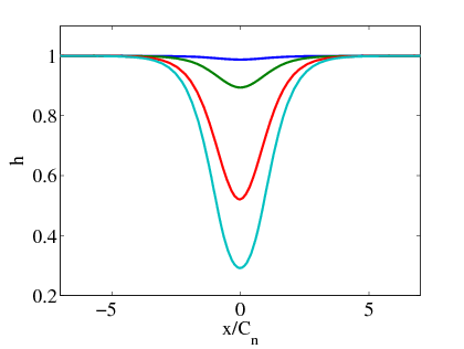
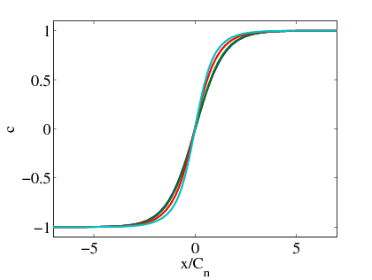
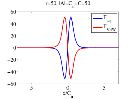
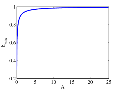
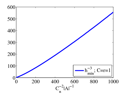
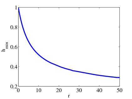
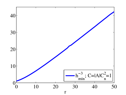
from the inequality , since is a local minimum. Thus, from Eq. (6.7b) we obtain the bound
| (6.8) |
The repulsive Van der Waals potential therefore has a regularizing effect on the solutions. We carried out a further numerical integration to find the general dependence of the magnitude of the dip on the parameters of Eq. (6.7b). There is no clear scaling law for this dependence, although the approximate rule is evidenced by Fig. 6.2, a relationship that is exact when , as seen in Eq. (6.4). Thus, we have characterized the equilibrium solution as fully as possible. We now consider the physical meaning of these results.
The formation of the valley in the height field has the physical interpretation of a balance between the Van der Waals and backreaction effects. From Fig. 6.1 (c) we see that the backreaction or capillary force and the Van der Waals force have opposite sign. The repulsive Van der Waals force acts like a nonlinear diffusion and inhibits rupture, and therefore promotes rupture, a result seen in experiments [39]. The valley in the height field therefore represents a balance between the smoothening and rupture-inducing effects.
We compare the no-rupture condition in Eq. (6.8) with the analytical results obtained in Ch. 5. In terms of the physical parameters of the system, the no-rupture condition of Ch. 5 is
where , and . The function has no explicit -dependence: although depends on , it is possible to find initial data to remove this dependence. We show a representative plot of in Fig. 6.3. Although a comparison between Fig. 6.2 and Fig. 6.3 is not exact, since the boundary conditions and domains are different in both cases, we see that the shape of the bound in Fig. 6.2 is different from that in Fig. 6.3. Since the bound in Fig. 6.2 is obtained from numerical simulations, and is intuitively correct, we conclude that it has the correct shape and that the bound of Fig. 6.3, while mathematically indispensable, is not sharp enough to be useful in determining the parametric dependence of the dip in free-surface height.
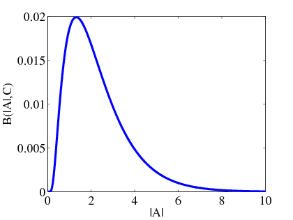
The procedure of identifying a phase-separating instability and studying non-trivial equilibrium solutions is recurrent in Cahn–Hilliard dynamics, and is discussed in Ch. 2. In that case, the nontrivial one-dimensional equilibrium solution hints at the late-time solution in several dimensions. Indeed, the one-dimensional antikink solution suggests that the late-time solution in several dimensions consists of domains with transition regions of the same width as the antikink width. Thus, we expect the equilibrium solution in Fig. 6.1 to reflect the late-time structure of a general phase-separating fluid in a thin film. This is found to be the case in one-dimensional, time-dependent numerical simulations, of which Fig. 6.4 is an example; here the concentration forms domains , separated by smooth transition regions, while the free-surface height forms peaks and valleys, with valleys occurring in the transition regions. The flatness of the peaks depends on the Van der Waals parameter , with large producing flat peaks, while the depth of the valleys depends on the value of the backreaction strength . The periodicity in Fig. 6.4 is due to the periodicity of the initial conditions, in particular the period-four initial condition for the height field. Purely random initial conditions give rise to a similar but aperiodic pattern of domains, peaks, and valleys.
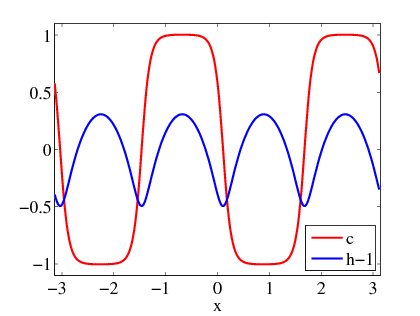
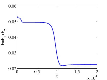
We have found by one-dimensional calculations, that the ultimate state of the equation system Eq. (1.1c) is a concentration field comprising domains, with a height profile that dips at domain boundaries. In order to pursue this claim further, and to examine the dynamics of domain growth, we turn to simulations in two dimensions.
6.3 Solutions in two dimensions
In this section we outline a numerical method for the two-dimensional thin-film Cahn–Hilliard equations and apply it in two distinct cases: constant surface tension only, and spatially-varying surface tension (or applied tangential stress). In each case, the regularizing Van der Waals potential is included to avoid film rupture. The introduction of appropriate structure functions enables us to measure the lengthscales of the concentration morphology.
To measure the typical scale of the domains we introduce a structure function in what follows. Because the concentration field is dependent only on the lateral coordinates and , we work in two dimensions only. Thus, as in Sec. 3.2 a measure of the correlation of concentration between two neighbouring points in Fourier space is given by the expression
where is the box size, and where denotes the spatial average. We normalize this function and compute its spherical average to obtain the structure function
where the spherical average any function is defined as
Hence is the spherical average of the Fourier coefficient . Thus we identify the dominant lengthscale with the reciprocal of the most important -value, defined as the first moment of the distribution ,
| (6.9) |
In performing the spherical average, we have assumed that the system is isotropic. If the isotropy is broken, for example, by the presence of an external shear flow, then a vector-valued measure of the domain lengthscales is given by
Using the initial conditions and the scale analysis we have outlined, we carry out the simulations for a variety of external conditions.
Numerical method
To simulate the thin-film SCH equations (6.1d), we use a semi-implicit finite-difference algorithm in two dimensions, although here we sketch the method in one dimension only. The height field is updated first, using semi-implicit finite differences [103]. The height field of Eq. (1.1c) is discretized in time as follows,
| (6.10) |
where
contains third-order derivatives and lower. Equation (6.10) is solved for using the Newton method for root-finding. Using the updated value of the height, we update the concentration, making use of the following discretization in time,
| (6.11) |
where
contains third-order derivatives and lower. Here is the velocity and is the chemical potential, defined in Sec. 5.2. Equation (6.11) is solved using a spectral method [5].
We solve the equations on a square grid with a timestep of , and the results do not change markedly upon increasing the resolution or decreasing the timestep. Following standard practice [16, 20, 71], the Cahn number is taken to be so that the transition region is just barely resolved. The boundary conditions are periodic in the lateral directions. The initial condition for the height field is a sinusoidal perturbation while the concentration field is given a random perturtion about zero. In contrast to the usual Cahn–Hilliard equation [71] however, the zero spatial mean of the concentration field does not persist, since it is the quantity , not that is conserved.
Constant surface tension
We let , and study the velocity field
| (6.12) |
We carry out simulations according to the scheme discussed above and find that the system evolves towards towards its late-time configuration in the following way. At early times, domains of like concentration start to form,
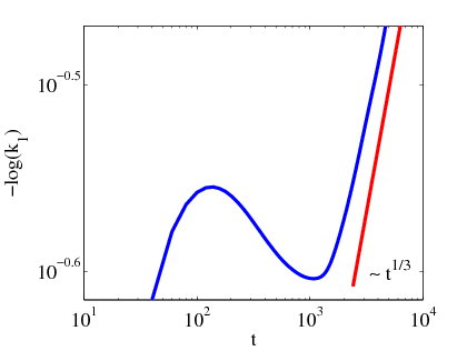
while the initial configuration of the free surface is destroyed due to nonlinear diffusive effects in the height equation. At later times, the domains continue to form and then to grow, while the free-surface height becomes slaved to the concentration field. That is, the spatial and temporal variations of the free surface depend on the concentration level. The free-surface height possesses local maxima in regions where domains of concentration have formed (peaks) while at the transition between domains of different binary fluid components, the free-surface height decreases markedly (valleys), as in the one-dimensional simulations of Sec. 6.2. The location of the surface peaks over the concentration domains has been seen in experiments involving polymeric thin films [104]. As in the case of ordinary Cahn–Hilliard dynamics, the late-time configuration selected is the one that tends to minimize the free energy. Now the free energy has the form
with , and the dynamics outlined do indeed decrease this free energy.
We characterize the growth of the domains by examining the function in Fig. 6.5. After transient effects have passed, the lengthscale
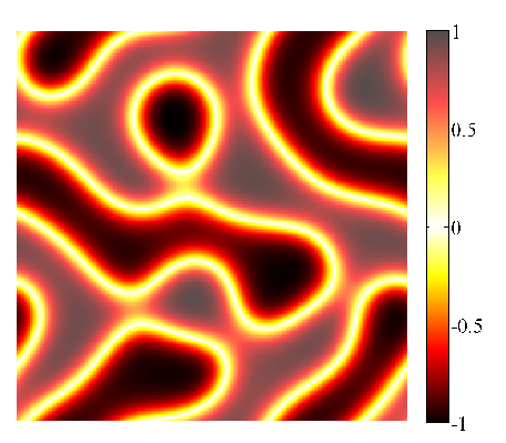
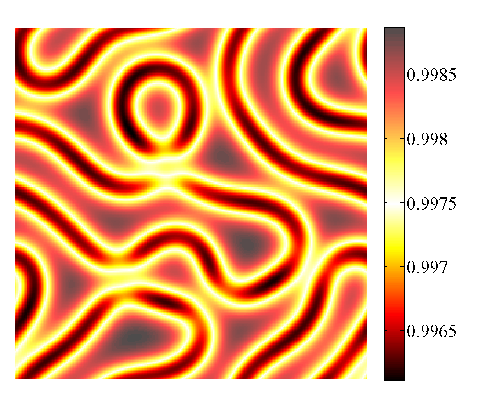
grows approximately as , which is the Lifshitz–Slyozov growth rate for phase separation in the absence of flow [48]. Several numerical simulations with different values of , , and , indicate that the scaling law is independent of these parameters. A better estimate of the growth law could be obtained by increasing the resolution, although this is computationally costly. However, the qualitative features of the system are well described by low-resolution simulations. The recovery of the growth law demonstrates that the Lifshitz–Slyozov mechanism of evaporation-condensation dominates over other effects, such as viscosity-driven phase separation [4]. This is not surprising, since the timescale that determined the asymptotic ordering in the derivation of Eq. (1.1c) was the diffusion time . In this sense, our model equations demonstrate the importance of variations in the free-surface height, rather than hydrodynamics. At very late times, the scaling rules are spoiled by finite-size effects.
Variable surface tension
We let , is a dimensionless amplitude, is the spatial scale of the surface tension variation, and is an integer. Then the velocity that drives the system becomes
| (6.13) |
By inspection of Eq. (5.3b), this velocity field may also be obtained by imposing a shear stress at the surface, provided . The imposed shear stress acts as a driving force.
This choice of velocity field leads to control of phase separation in the following manner. For small values of the backreaction strength, with , the height field quickly aligns with the surface tension profile as in Fig. 6.9,
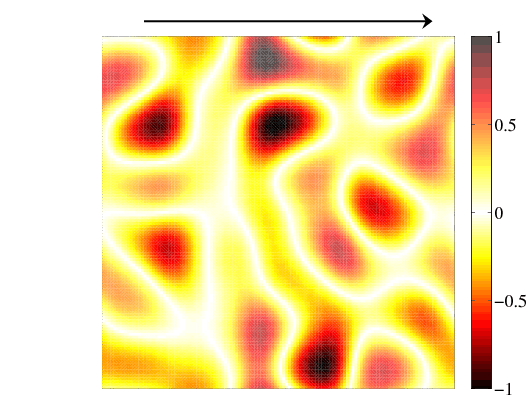
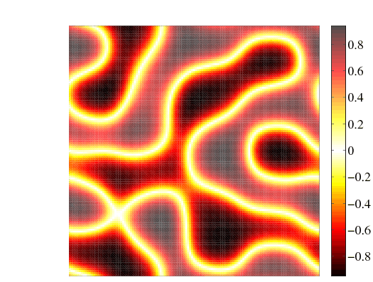
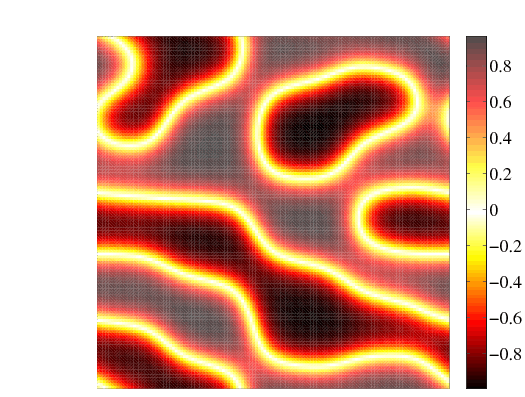
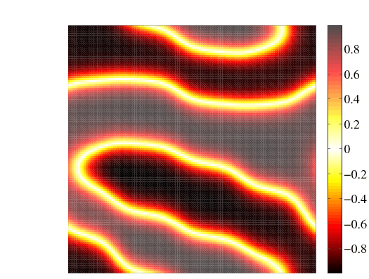
since the strong effect of the Van der Waals diffusion destroys the unforced part of . At the same time, the concentration field begins to form domains. At later times, when , the domains align with the gradient of the forcing term. The growth of the domains continues in this direction and is arrested (or slowed down considerably) in the direction perpendicular to the forcing. The domains are string-like, with kinks occurring along lines where is minimized, as evidenced by Fig. 6.7. The decay of and is shown in Fig. 6.10. It is not clear whether the decay of is arrested or continues slowly, and we do not report the decay rate here.
For moderate values of the backreaction strength with , the height field again assumes a profile aligned with the surface tension, while domains of concentration now align in a direction perpendicular to the forcing gradient. Domain growth
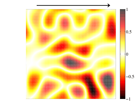
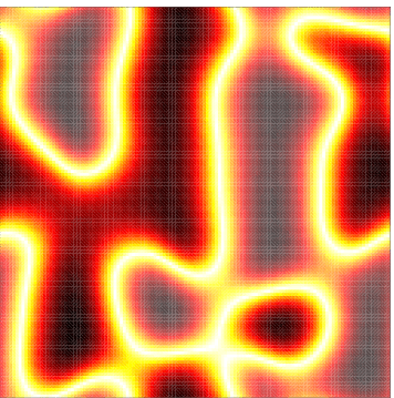
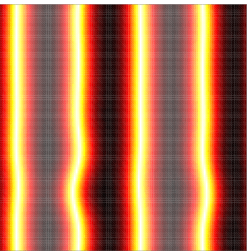
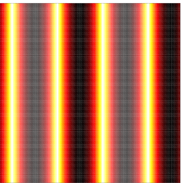
continues in the perpendicular direction and is arrested in the direction of the driving-force gradient. A pattern of string-like domains emerges, with domain boundaries forming along lines where both and are maximized. Eventually, the domain boundaries align perfectly with the surface tension maxima, as evidenced in Fig. 6.8.
The control of phase separation therefore depends crucially on the backreaction. This result is amplified by the existence of a no-rupture condition only for the case, where there is no backreaction. This condition relies on the alignment of the height and surface tension profiles, which is exact
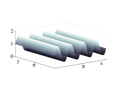
only when the backreaction is zero. Then at late times, the system evolves towards equilibrium and is described by the steady state , which by the alignment property reduces to the one-dimensional equation
| (6.14) |
By multiplying both sides of the expression by , differentiating and then evaluating the result at , a coincident minimum of height and surface tension, we obtain the condition
Since is a minimum of height, , which prevents from being zero. On the other hand, for and sufficiently large, the alignment of height and surface tension profiles is not exact, the reduction of the steady-state condition to Eq. (6.14) is no longer possible, and our calculation fails. In that case, simulations show that the film ruptures in finite time.
We have outlined, by numerical simulations and calculations, three possible outcomes for the phase separation, depending on the backreaction
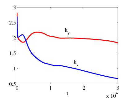
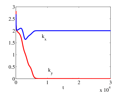
strength . For , the concentration forms string-like domains, aligned with the applied force. For the concentration forms domains that align perfectly in a direction perpendicular to the applied force, while for , the forcing causes the film to rupture. Loosely speaking, the different regimes occur because for the concentration field couples to the gradient , while for , the concentration field couples to the patterned surface tension . Thus, the interfacial tension or backreaction can therefore be tuned to achieve the desired outcome.
6.4 Summary
We have derived a thin-film model of phase separation based on the NSCH equations, in which the reaction of concentration gradients on the flow is important. We have used this model to give a qualitative picture of the features of phase separation in real thin films, in particular the tendency of concentration gradients to promote rupture in the film, and to produce peaks and valleys in the free surface that mirror the underlying domain morphology. We have found that in the presence of a unidirectional sinusoidal variation in surface tension, the strength of the backreaction determines the direction in which the domains align. This result could prove useful in microfabrication applications where control of phase separation is required [37].
Because the lubrication model suppresses vertical variations in the concentration field, we are limited to the case where the binary fluid components interact identically with the boundaries at the substrate and free surface. However, the model quite generally gives an accurate description of surface roughening arising from Van der Waals forces. More detailed models based on this approach, involving different boundary conditions that better reflect wetting behaviour and a concentration-dependent Hamakar coefficient, could capture a wider range of thin-film behaviour, although the tradeoff could be a loss of mathematically interesting features, such as the Lyapunov functional.
Chapter 7 Singular solutions of aggregation equations
7.1 Overview
In this chapter we introduce a generalized gradient flow equation that serves as a bridge from the Cahn–Hilliard theory we have discussed, to models of aggregation that are currently used in nanoscale physics. We then focus on a particular aggregation model that describes a nonlocal magnetic system and admits singular solutions that emerge from smooth initial data. The magnetic system comprises a Gilbert-type equation for an orientation vector, and a scalar density equation. We study the uncoupled Gilbert-type equation and find that the evolution depends strongly on the lengthscales of the nonlocal effects. We then pass to a coupled density-magnetization model and perform a linear stability analysis, noting the effect of the lengthscales of nonlocality on the system’s stability properties. We carry out numerical simulations of the coupled system and find that singular solutions emerge from smooth initial data. The singular solutions represent a collection of interacting particles (clumpons). By restricting ourselves to the two-clumpon case, we are reduced to a two-dimensional dynamical system that is readily analyzed, and thus we classify the different clumpon interactions possible.
7.2 Gradient flow, variable mobility, and nonlocality
In this section we introduce a generalized aggregation equation that includes the Cahn–Hilliard, Keller–Segel, and (scalar) Holm–Putkaradze equations as special cases.
Recall that the Cahn–Hilliard equation for an order parameter is derived from the gradient of a free-energy functional in dimensions,
where is a potential with two stable minima. In the previous chapters, we chose the double-well potential , and this choice simplified the analysis of the model. However, any potential with two stable minima and one unstable maximum will do. Therefore, in this chapter, we choose to work with the so-called double-obstacle potential
where is a positive parameter and the function is minus the system’s entropy density. Recall that the quartic double well was invariant under the component relabelling transformation . The logarithmic double well function has a similar symmetry: it is invariant under the relabelling transformation . We can now write down the Cahn–Hilliard equation in nonlocal form,
where is the kernel whose Fourier transform is
It is possible to prescribe a different kernel: other choices can lead to anisotropic or nonlocal interactions between fluid particles. Let us therefore examine the possibility of nonlocal interactions, and leave the kernel unspecified. We shall, however, restrict to central interactions, . The free energy functional is thus
| (7.1) |
As discussed in Ch. 2, the simplest rotationally-invariant, mass-preserving evolution equation that decreases this free energy is the gradient flow equation
where is a nonnegative function called the mobility and is the chemical potential. This evolution decreases the free energy:
The mobility function controls the strength of the particle diffusion and depends on the local density of the fluid. If the evolution is to respect the component relabelling symmetry, then the mobility must be a function of the combination . The simplest possible choice of mobility is thus
The evolution of the system preserves the positivity of this function because the energy cost of attaining the either of the states is infinite, as expressed in Eq. (7.1).
The nonlocal Cahn–Hilliard concentration for the concentration is thus
| (7.2) |
By specifying a particular kernel, or by modifying the mobility, we recover a number of models of aggregation. In particular,
-
•
If the Fourier transform of the kernel is , we recover the Cahn–Hilliard equation with the double-obstacle potential and variable mobility;
-
•
If the Fourier transform of the kernel is , where is the lengthscale of the potential energy , that is, if is the kernel of the Helmholtz operator , we recover the regularized Keller–Segel equation***The regularized Keller–Segel equation is discussed in Appendix B;
-
•
If is any nonlocal kernel, , and the mobility is replaced with , where is the smoothened density
we obtain the scalar Holm–Putkaradze model [38].
The scalar Holm–Putkaradze model was introduced in [38, 66] and describes the evolution of a single scalar density. In particular, given the (negative) free energy
the model admits singular solutions that emerge from smooth initial data. The singular solutions satisfy a set of ordinary differential equations. The model can therefore be used to describe self-assembly in nanoscale physics, in which atoms or molecules aggregate to from larger, mesoscale structures with particle-like properties. These particles are governed by the ordinary differential equations to which the aggregation equation reduces. The aggregation equation (7.2) that we have formulated thus provides a bridge from the Cahn–Hilliard theory we have discussed, to this more recent application in nanoscale physics. The authors Holm, Putkaradze, and Tronci have extended this model to a coupled scalar-vector system in [62], although they simply formulate the equations, and do not examine the properties of the model in any detail. Therefore, using the numerical tools that we have developed, and our knowledge of aggregation through energy minimization, we turn to this coupled scalar-vector system, and provide qualitative and quantitative descriptions of its behaviour.
We treat the initial state of the system as a continuum, a good approximation in nanophysics applications [105]. One realization of this problem is in nanoscale magnetic systems, in which particles with a definite magnetic moment collapse and form mesoscale structures, that in turn have a definite magnetic moment. Thus, in this chapter we refer to the orientation vector in our continuum picture as the magnetization.
7.3 The nonlocal Gilbert equation
In this section we study a magnetization equation that in form is similar to the Gilbert equation, that is, the Landau–Lifshitz–Gilbert equation in the over-damped limit [106, 107]. The equation we focus on incorporates nonlocal effects, and was introduced in [62]. We study the evolution and energetics of this equation, and examine the importance of the problem lengthscales in determining the evolution.
We study the following nonlocal Gilbert (NG) equation
| (7.3) |
where the magnetization vector , its smoothened version , and the variational derivative are functions of the form
The smoothened magnetization is defined as
and is prescribed as follows,
The smoothened magnetization and the force can be computed using the theory of Green’s functions. In particular,
Here denotes the convolution of functions, and the kernel satisfies the equation
| (7.4) |
The function is the Dirac delta function. Equation (7.4) is solved subject to conditions imposed on the boundary of the domain . In this chapter we shall work with a periodic domain or , although other boundary conditions are possible. Since , is a simultaneous eigenfunction of the operators and , equation (7.3) has a family of nontrivial equilibrium states given by
where is a constant vector, is some wavenumber, and is a constant phase. The derivation of this solution is subject to the boundary conditions discussed in Sec. 7.4.
By setting and replacing with , we recover the more familiar Landau–Lifshitz–Gilbert equation, in the overdamped limit [106],
| (7.5) |
Equation (7.3) possesses several features that will be useful in understanding the numerical simulations. There is an energy functional
| (7.6) |
which evolves in time according to the relation
| (7.7) | |||||
This is not necessarily a nonincreasing function of time, although setting gives
| (7.8) | |||||
where is the angle between and . In the special case when , we therefore expect to be a nonincreasing function of time. On the other hand, inspection of Eq. (7.7) shows that as , the energy tends to a constant. Additionally, the magnitude of the vector is conserved. This can be shown by multiplying Eq. (7.3) by , and by exploiting the antisymmetry of the cross product. Thus, we are interested only in the orientation of the vector ; this can be parametrized by two angles on the sphere:
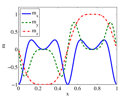
the azimuthal angle , and the polar angle , where
| (7.9) |
and where , and .
We carry out numerical simulations of Eqs. (7.3) and (7.5) on a periodic domain , and outline the findings in what follows. Motivated by the change of coordinates (7.9), we choose the initial data
| (7.10) |
where and are integers. These data are shown in Fig. 7.1.
Case 1: Numerical simulations of Eq. (7.5). Equation (7.5) is usually solved by explicit or implicit finite differences [107]. We solve the equation by these methods, and by the explicit spectral method [5]. The accuracy and computational cost is roughly the same in each case, and for simplicity, we therefore employ explicit finite differences; it is this method we use throughout the chapter. Given the initial conditions (7.10), each component of the magnetization tends to a constant, the energy
decays with time, and retains its initial value . After some transience, the decay of the energy functional becomes exponential in time. These results are shown in Fig. 7.2
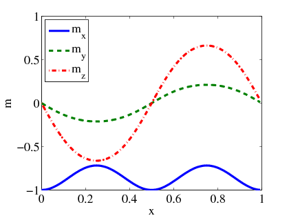

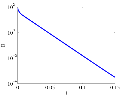
Case 2: Numerical simulations of Eq. (7.3) with . Given the smooth initial data (7.10), in time each component of the magnetization decays to zero, while the energy
tends to a constant value. Given our choice of initial conditions, the energy in fact increases to attain this constant value. Again the quantity stays constant. These results are shown in Fig. 7.3. We find similar results when we set .
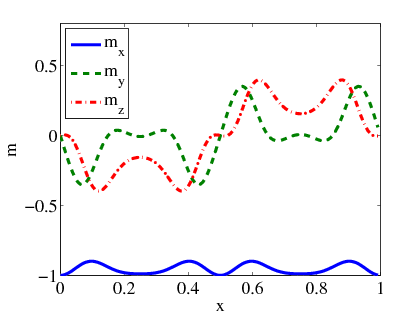
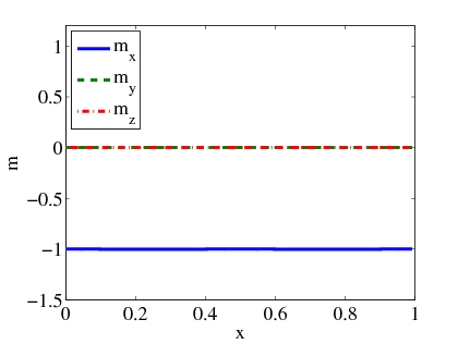
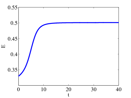
Case 3: Numerical simulations of Eq. (7.3) with . Given the smooth initial data (7.10), in time each component of the magnetization develops finer and finer scales. The development of small scales is driven by the decreasing nature of the energy functional, which decreases as power law at late times, and is reflected in snapshots of the power spectrum of the magnetization vector, shown in Fig. 7.4. As the system evolves, there
| Case | Lengthscales | Energy | Outcome as | Linear Stability |
|---|---|---|---|---|
| , | ||||
| (1) | Decreasing | Constant state | Stable | |
| (2) | Increasing | Constant state | Stable | |
| Development of finer | ||||
| (3) | Decreasing | and finer scales | Unstable |
is a transfer of large amplitudes to higher wavenumbers. This transfer slows down at late times, suggesting that the rate at which the solution roughens tends to zero, as . The evolution preserves the symmetry of the magnetization vector under parity transformations. This is seen by comparing Figs. 7.1 and 7.4. The energy is a decaying function of time, while the quantity stays constant. We find similar results for the case when .
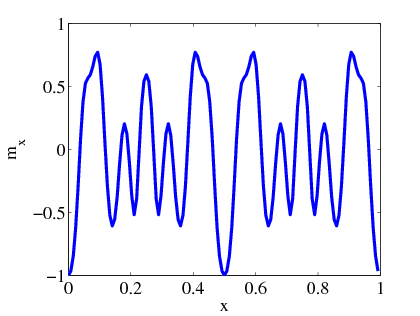
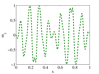
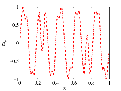
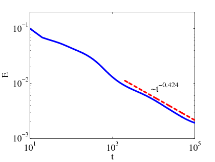
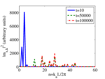
These results can be explained qualitatively as follows. In Case (1), the energy functional exacts a penalty for the formation of gradients. The energy decreases with time and the system evolves into a state in which no magnetization gradients are present, that is, a constant state. On the other hand, we have demonstrated that in Case (2), when , the energy increases to a constant value. Since in the nonlocal model, the energy functional represents the cost of forming smooth spatial structures, an increase in energy produces a smoother magnetization field, a process that continues until the magnetization reaches a constant value. Finally, in Case (3), when , the energy functional decreases, and this decrease corresponds to a roughening of the magnetization field, as seen in Fig. 7.4. In Sec. 7.4 we shall show that Case (2) is stable to small perturbations around a constant state, while Case (3) is unstable. These results are summarized in Table 7.1.
The solutions of Eqs. (7.3) and (7.5) do not become singular. This is not surprising: the manifest conservation of in Eqs. (7.3) and (7.5) provides a pointwise bound on the magnitude of the solution, preventing blow-up. Any addition to Eq. (7.3) that breaks this conservation law gives rise to the possibility of singular solutions, and it is to this possility that we now turn.
7.4 Coupled density-magnetization equations
In this section we study a coupled density-magnetization equation pair that admit singular solutions. We investigate the linear stability of the equations and examine the conditions for instability. We find that the stability or otherwise of a constant state is controlled by that state’s magnetization and density, and by the relative magnitude of the problem lengthscales. Using numerical and analytical techniques, we investigate the emergence and self-interaction of singular solutions.
The equations we study are as follows,
| (7.11a) | |||
| (7.11b) |
where we set
and, as before,
The order parameter has the interpretation of a particle density, while the orientation vector has the interpretation of a local magnetization field. These equations have been introduced by Holm, Putkaradze and Tronci in [62], using a kinetic-theory description. The density and the magnetization vector are driven by the velocity
| (7.12) |
The velocity advects the ratio by
We have the system energy
| (7.13) |
and, given a nonnegative density, the second term is always nonpositive. This represents an energy of attraction, and we therefore expect singularities in the magnetization vector to arise from a collapse of the particle density due to the ever-decreasing energy of attraction. There are three lengthscales in the problem that control the time evolution: the ranges and of the potentials in Eq. (7.13), and the smoothening length .
Linear stability analysis
We study the linear stability of the constant state . We evaluate the smoothened values of this constant solution as follows,
For periodic or infinite boundary conditions, the constants and are in fact zero and thus
| (7.14) |
and similarly . The result (7.14) guarantees that the constant state is indeed a solution of Eq. (7.11b).
We study a solution , which represents a perturbation away from the constant state. By assuming that and are initially small in magnitude, we obtain the following linearized equations for the perturbation density and magnetization,
| (7.15) | |||
For we may choose two unit vectors and such that , and form an orthonormal triad (that is, we have effected a change of basis). We then study the quantities , , and , where
We obtain the linear equations
By focussing on a single-mode disturbance with wavenumber we obtain the following system of equations
with eigenvalues
| (7.16) |
The eigenvalues are the growth rate of the disturbance [108]. There are two routes to instability, when , or when . The first route leads to an instability when
while the second route leads to instability when
We have plotted the growth rates for the case when , and compared the theory with numerical simulations. There is excellent agreement at low wavenumbers, although the numerical simulations become less accurate at high wavenumbers. This can be remedied by increasing the resolution of the simulations. These plots are shown in Figs. 7.5 and 7.6.
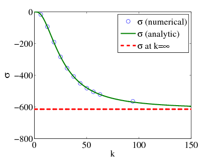
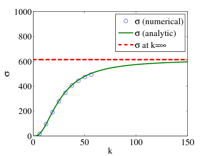
The growth rates are parabolic in at small ; saturates at large , while attains a maximum and decays at large . The growth rates can be positive or negative, depending on the initial configuration, and on the relationship between the problem lengthscales. In contrast to some standard instabilities of pattern formation (e.g. Cahn–Hilliard (Sec. 2.2) or Swift–Hohenberg [109]), the -unstable state becomes more unstable at higher wavenumbers (smaller scales), thus preventing the ‘freezing-out’ of the instability by a reduction of the box size [110]. The growth at small scales is limited,
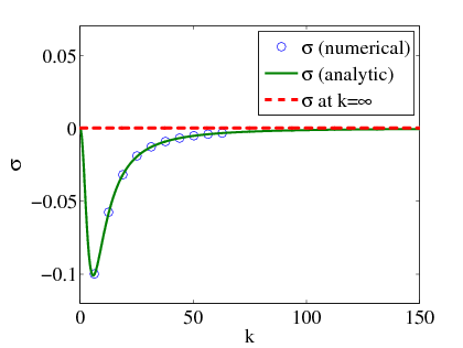
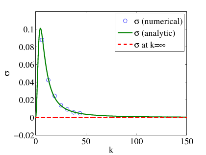
however, by the saturation in as . Heuristically, this can be explained as follows: at higher wavenumber, the disturbance gives rise to more and more peaks per unit length. This makes merging events increasingly likely, so that peaks combine to form larger peaks, enhancing the growth of the disturbance.
Recall in Sec. 7.3 that the different behaviours of the magnetization equation (7.3) are the result of a competition between the lengthscales and . For the initial (large-amplitude) disturbance tends to a constant, while for the initial disturbance develops finer and finer scales. In this section, we have shown that the coupled density-magnetization equations are linearly stable when , while the reverse case is unstable. In contrast to the first route to instability, the growth rate , if positive, admits a maximum. This is obtained by setting . Then the maximum growth rate occurs at a scale
Thus, the scale at which the disturbance is most unstable is determined by the geometric mean of and . Given a disturbance with a range of modes initially present, the instability selects the disturbance on the scale . This disturbance develops a large amplitude and a singular solution subsequently emerges. It is to this aspect of the problem that we now turn.
Singular solutions
In this section we show that a finite weighted sum of delta functions satisfies the partial differential equations (7.11b). Each delta function has the interpretation of a particle or clumpon, whose weights and positions satisfy a finite set of ordinary differential equations. We investigate the two-clumpon case analytically and show that the clumpons tend to a state in which they merge, diverge, or are separated by a fixed distance. In each case, we determine the final state of the two clumpons’ relative orientation.
To verify that singular solutions are possible, let us substitute the ansatz
| (7.17) |
into the weak form of equations (7.11b). Here we sum over the different components of the singular solution (which we call clumpons). In this section we work on the infinite domain . The weak form of the equations is obtained by testing Eqs. (7.11b) with once-differentiable functions and ,
| (7.18a) | |||
| (7.18b) |
Substitution of the ansatz (7.17) into the weak equations (7.18b) yields the relations
| (7.19) |
where and are obtained from the ansatz (7.17) and are evaluated at . Note that the density weights and the magnitude of the weights remain constant in time.
We develop further understanding of the clumpon dynamics by studying the two-clumpon version of Eqs. (7.19). Since the weights , , , and are constant, two variables suffice to describe the interaction: the relative separation of the clumpons, and the cosine of the angle between the clumpon magnetizations, . Using the properties of the kernel , , we derive the equations
| (7.20a) | |||
| (7.20b) |
where , , and are constants. In this framework, is the Green’s function of the Helmholtz operator , . Equations (7.20b) form a dynamical system whose properties we now investigate using phase-plane analysis [111]. We note first
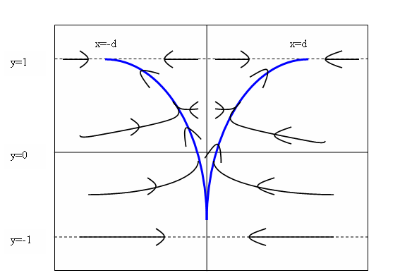
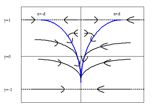
of all that the region of the phase plane is forbidden, since the -component of the vector field vanishes at . The vertical lines and are equilibria, although
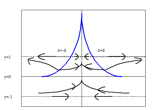
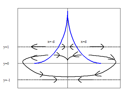
their stability will depend on the value of the parameters . The curve across which changes sign is called the nullcline. This is given by
which on the domain takes the form
Several qualitatively different behaviours are possible, depending on the
| Case | vs. | vs. | Equilibria | Flow |
|---|---|---|---|---|
| ; | Flow into and | |||
| (1) | ; | |||
| Flow into and | ||||
| (2) | ; | |||
| ; | Flow into | |||
| (3) | ; | and | ||
| ; | Flow into | |||
| (4) | ; | and |
magnitude of the values taken by the parameters . Here we outline four of these behaviour types.
-
•
Case 1: The lengthscales are in the relation , and . The nullcline is shown in Fig. 7.7. There is flow into the fixed points , and into the line , while is a nondecreasing function of time, which follows from Eq. (7.20b). The ultimate state of the system is thus , (alignment), or (merging). In the latter case the final orientation is given by the integral of Eq. (7.20b),
(7.21) -
•
Case 2: The lengthscales are in the relation , , and the nullcline is the same as Case (2). All flow along the line is directed towards the fixed points . All other initial conditions flow into the line , since is now a nonincreasing function of time. The ultimate state of the system is thus , (alignment), or (merging). In the latter case the final orientation is given by the formula (7.21).
-
•
Case 3: The lengthscales are in the relation and . The nullcline is shown in Fig. 7.8. Inside the region bounded by the line and the nullcline, the flow is into the line (merging), and the fixed points are unstable. The flow below the line is towards the line . Outside of these regions, however, the flow is into the lines , which shows that for a suitable choice of parameters and initial conditions, the clumpons can be made to diverge.
-
•
Case 4: The lengthscales are in the relation and , and the nullcline is the same as Case (3). The quantity is a nonincreasing function of time. All flow along the line is directed away from the fixed points and is into the fixed points , or . All other initial conditions flow into , although initial conditions that start above the curve formed by the nullcline flow in an arc and eventually reach a fixed point .
We summarize the cases we have discussed in Table 7.2. Using numerical simulations of Eqs. (7.20b), we have verified that Cases (1)–(4) do indeed occur. The list of cases we have considered is not exhaustive: depending on the parameters , , and , other phase portraits may arise. Indeed, it is clear from Fig. 7.7 that through saddle-node bifurcations, the fixed points may disappear, or additional fixed points may appear. Our analysis shows, however, that it is possible to choose a set of parameters such that two clumpons either merge, diverge, or are separated by a fixed distance.
Numerical Simulations
To examine the emergence and subsequent interaction of the clumpons, we carry out numerical simulations of Eq. (7.11b) for a variety of initial conditions. We use an explicit finite-difference algorithm with a small amount of artifical diffusion. We solve the following weak form of Eq. (7.11b), obtained by testing Eq. (7.18b) with ,
where and is the unit vector in the direction. We work on a periodic domain , at a resolution of gridpoints; going to higher resolution does not noticeably increase the accuracy of the results.
The first set of initial conditions we study is the following,
| (7.22) |
where , , and are random phases in the interval , and is the fundamental wavenumber. The initial conditions for the magnetization vector are chosen to represent the lack of a preferred direction in the problem. The time evolution of equations (7.11b) for this set of initial conditions is shown in Fig. 7.9. After a short time, the initial data become singular, and subsequently, the solution can be represented as a sum of clumpons,
Here is the number of clumpons present at the singularity time. This number corresponds to the number of maxima in the initial density profile. The forces exerted by each clumpon on the other balance because of the effect of the periodic boundary conditions. Indeed, any number of equally-spaced, identical, interacting particles arranged on a ring are in equilibrium, although this equilibrium is unstable for an attractive force. Thus, at late times, the clumpons are stationary, while the magnetization vector shows alignment of clumpon magnetizations.
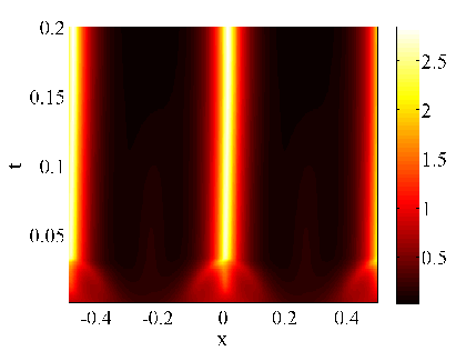
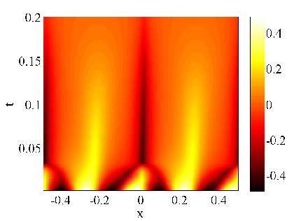
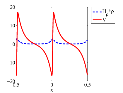
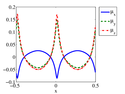
We gain further understanding of the formation of singular solutions by studying the system velocity just before the onset of the singularity. This is done in Fig. 7.10. Figure 7.10 (a) shows the development of the two clumpons from the initial data. Across each density maximum, the velocity has the profile , where is an increasing function of time. This calls to mind the advection problem for the scalar , studied by Batchelor in the context of passive-scalar mixing [92]
Given initial data , the solution evolves in time as
so that gradients are amplified exponentially in time,
in a similar manner to the problem studied.
The evolution of the set of initial conditions (7.22) has therefore demonstrated the following: the local velocity is such that before the onset of the singularity, matter is compressed into regions where is large, to such an extent that the matter eventually accumulates at isolated points, and the singular solution emerges. Moreover, the density maxima, rather than the magnetization extrema, drive the formation of singularities. This is not surprising, given that the attractive part of the system’s energy comes from density variations.
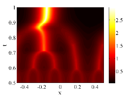
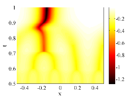
To highlight the interaction between clumpons, we examine the following set of initial conditions,
| (7.23) |
where is the fundamental wavenumber. Since this set of initial conditions contains a large number of density maxima, we expect a large number of closely-spaced clumpons to emerge, and this will illuminate the clumpon interactions. The time evolution of equations (7.11b) for this set of initial conditions is shown in Fig. 7.11. As before, the solution becomes singular after a short time, and is subsequently represented by a sum of clumpons,
Here is the number of clumpons at the singularity time. This number corresponds to the number of maxima in the initial density profile. As before, this configuration of equally spaced, identical clumpons is an equilibrium state, due to periodic boundary conditions. Therefore, once the particle-like state has formed, we impulsively shift the clumpon at by a small amount, and precipitate the merging of clumpons. The eight clumpons then merge repeatedly until only a single clumpon remains. The tendency for the clumpons to merge is explained by the velocity , which changes sign across a clumpon. Thus, if a clumpon is within the range of the force exerted by its neighbours, the local velocity, if unbalanced, will advect a given clumpon
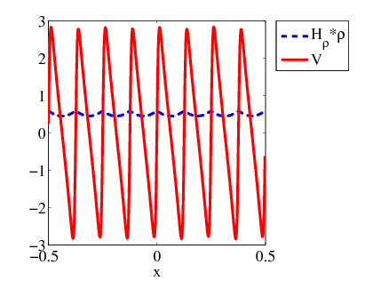
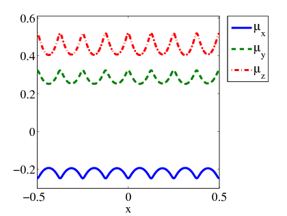
in the direction of one of its neighbours, and the clumpons merge. This process is shown in Fig. 7.13.
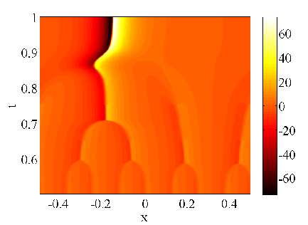
7.5 Summary
We have investigated the nonlocal Gilbert (NG) equation introduced by Holm, Putkaradze, and Tronci in [62] using a combination of numerical simulations and simple analytical arguments. The NG equation contains two competing lengthscales of nonlocality: there is a lengthscale associated with the range of the interaction potential, and a lengthscale that governs the smoothened magnetization vector that appears in the equation. When all initial configurations of the magnetization tend to a constant value, while for the initial configuration of the magnetization field develops finer and finer scales. These two effects are in balance when , and the system does not evolve away from its initial state. Furthermore, the NG equation conserves the norm of the magnetization vector , thus providing a pointwise bound on the solution and preventing the formation of singular solutions.
To study the formation of singular solutions, we couple the NG equation to a scalar density equation. Associated with the scalar density is a negative energy of attraction that drives the formation of singular solutions and breaks the pointwise bound on the . Three lengthscales of nonlocality now enter into the problem: the range of the force associated with the scalar density, the range of the force due to the magnetization, and the smoothening length. As before, the competition of lengthscales is crucial to the evolution of the system; this is seen in the linear stability analysis of the coupled equations, in which the relative magnitude of the lengthscales determines the stability or otherwise of a constant state.
Using numerical simulations, we have demonstrated the emergence of singular solutions from smooth initial data, and have explained this behaviour by the negative energy of attraction produced by the scalar density. The singular solution consists of a weighted sum of delta functions, given in Eq. (7.17), which we interpret as interacting particles or clumpons. The clumpons evolve under simple finite-dimensional dynamics. We have shown that a system of two clumpons is governed by a two-dimensional dynamical system that has a multiplicity of steady states. Depending on the lengthscales of nonlocality and the clumpon weights, the two clumpons can merge, diverge, or align and remain separated by a fixed distance.
Chapter 8 Conclusions
The advective Cahn–Hilliard equation, describing the twin effects of advection and phase separation, has been the subject of this report. We have considered cases with and without feedback from concentration gradients into the advecting flow field.
In Ch. 2 we introduced the theory necessary for the report, and one new result: an existence theory for the passively-advected Cahn–Hilliard equation. Although an important exercise, such existence theories generally tell us no more than the regularity class to which the solution belongs. Therefore, we resorted to numerical simulations in Ch. 3, considering phase separation in the presence of a passive, chaotic flow. We characterized the model random-phase sine flow by its Lyapunov exponent and correlation length. We quantified the phase separation using the morphology, lengthscales, and probability distribution function of the concentration field. We showed how a chaotic flow will not only arrest the growth of the phase-separated domain structure, but will lead to remixing of the binary fluid. We highlighted the importance of this result in applications where the coarsening tendency of the binary fluid is undesirable.
Continuing in this vein, in Ch. 4 we defined what it means for a symmetric binary fluid to be well mixed and, given a smooth stirring velocity, and sources and sinks, we obtained very precise bounds on the level of mixedness achievable by the flow. The question then arises, given a certain source term, is there a best flow for mixing a binary fluid? Unlike in the theory of miscible liquids, we could not give a complete answer, but noted that the random-phase sine flow of Ch. 3 is efficacious, but not necessarily optimal, at mixing.
In Ch. 5, we switched focus to the active Cahn–Hilliard equation, which is coupled to the Navier–Stokes equations. By specializing to the case where the binary fluid forms a thin layer on a substrate, it was possible to obtain new, coupled equations, describing the coevolution of the film’s free-surface height and the fluid concentration, the so-called Stokes Cahn–Hilliard equations. Since we were interested in the late-time behaviour of the system, we focussed on the cases where film rupture was impossible, by introducing a repulsive Van der Waals force. In that case, we obtained existence, regularity, and uniqueness results for solutions to the Stokes Cahn–Hilliard equations in two dimensions, and then passed over to numerical simulations in two and three dimensions in Ch. 6. The most salient result of this chapter was obtained by applying a spatially-varying surface tension across the film. Then, for moderate backreaction strengths, the binary fluid domains aligned with the direction of this variation, while for zero backreaction, the domains aligned in the perpendicular direction. This surprising result highlights the importance of coupled models, and gives a means of controlling phase separation.
In Ch. 7 we formulated a general theory of aggregation equations that includes as special cases the Cahn–Hilliard, Keller–Segel, and (scalar) Holm–Putkaradze equations. Motivated by this link between the theory we have developed and the nanoscale physics described by the Holm–Putkaradze equation, we studied a coupled vector-scalar system of aggregation equations that describes the formation of magnetic nanoparticles. Although this system was introduced by Holm, Putkaradze, and Tronci in [62], its properties had yet to be studied. Therefore, using numerical and analytical techniques, we highlighted the competition of lengthscales in a purely magnetic system, and demonstrated that singular solutions are never possible in such a model. By passing to the coupled vector-scalar model, we demonstrated the emergence of singular solutions from smooth initial data. We obtained a set of ordinary differential equations satisified by the discrete elements of the singular solution (clumpons). By focussing on the two-clumpon case, we showed rigorously that the two clumpons can merge, diverge, or align and remain at a fixed distance. We thus gave a full characterization of the Holm–Putkaradze–Tronci model of nanomagnetic particles.
There are many avenues for future work. The advective Cahn–Hilliard equation could be used to give a full picture the breakup and coalescence of droplets with high surface tension, an area in which there are many experiments but little theory, while more work could be done in finding an optimal flow for mixing the binary fluid. Computational topology [112] could be used to give an extra dimension to the characterization of concentration morphology in the presence of flow. On the other hand, more experiments on and modelling of the thin-film problem would shed further light on this aspect of NSCH dynamics. The relevance of Cahn–Hilliard and thin-film type equations to the theory of self-assembly could be probed further. It is the author’s hope to work on at least some of these problems in the future.
Bibliography
- [1] M. Lipman. Ireland: land of charm, humour, breathtaking vistas… and delicious homemade mayonnaise? The Guardian, 21st August 2006.
- [2] J. W. Cahn and J. E. Hilliard. Free energy of a nonuniform system. I. Interfacial energy. J. Chem. Phys, 28:258–267, 1957.
- [3] A. Karim, J. F. Douglas, L. P. Sung, and B. D. Ermi. Self-assembly by phase separation in polymer thin films. Encyclopedia of Materials: Science and Technology, page 8319, 2002.
- [4] A. J. Bray. Theory of phase-ordering kinetics. Adv. Phys., 43:357–459, 1994.
- [5] J. Zhu, L. Q. Shen, J. Shen, V. Tikare, and A. Onuki. Coarsening kinetics from a variable mobility Cahn–Hilliard equation: Application of a semi-implicit Fourier spectral method. Phys. Rev. E, 60:3564–3572, 1999.
- [6] C. M. Elliott and S. Zheng. On the Cahn–Hilliard equation. Arch. Rat. Mech. Anal., 96:339–357, 1986.
- [7] H. Gajewski and K. Zacharias. On a nonlocal phase separation model. J. Math. Anal. Appl., 286:11–31, 2003.
- [8] C. M. Elliott and H. Garcke. The Cahn–Hilliard equation with degenerate mobility. SIAM J. Math. Anal., 27:403–423, 1996.
- [9] Z. Shou and A. Chakrabarti. Ordering of viscous liquid mixtures under a steady shear flow. Phys. Rev. E, 61:R2200, 2000.
- [10] L. Berthier. Phase separation in a homogeneous shear flow: Morphology, growth laws, and dynamic scaling. Phys. Rev. E, 63:051503, 2001.
- [11] T. Hashimoto, K. Matsuzaka, and E. Moses. String phase in phase-separating fluids under shear flow. Phys. Rev. Lett., 74:126, 1995.
- [12] A. J. Bray. Coarsening dynamics of phase-separating systems. Phil. Trans. R. Soc. Lond., 361:781–792, 2003.
- [13] H. Aref. Stirring by chaotic advection. J. Fluid Mech., 143:1–21, 1984.
- [14] Jean-Pierre Eckmann and David Ruelle. Ergodic theory of chaos and strange attractors. Rev. Mod. Phys., 57(3):617–656, July 1985.
- [15] Stephen Wiggins. Introduction to Applied Dynamical Systems and Chaos. Springer-Verlag, New York, second edition, 2003.
- [16] L. Berthier, J. L. Barrat, and J. Kurchan. Phase separation in a chaotic flow. Phys. Rev. Lett., 86:2014–2017, 2001.
- [17] A. M. Lacasta, J. M. Sancho, and F. Sagues. Phase separation dynamics under stirring. Phys. Rev. Lett., 75:1791, 1995.
- [18] G. I. Taylor. Diffusion by continuous movement. Proc. London Math. Soc., 20:196–212, 1921.
- [19] J. Lowengrub and L. Truskinowsky. Quasi-incompressible Cahn–Hilliard fluids and topological transitions. Proc. R. Soc. Lond. A, 454:2617–2654, 1998.
- [20] S. Berti, G. Boffetta, M. Cencini, and A. Vulpiani. Turbulence and coarsening in active and passive binary mixtures. Phys. Rev. Lett., 95:224501, 2005.
- [21] D. J. Pine, N. Easwar, J. V. Maher, and W. I. Goldburg. Turbulent suppression of spinodal decomposition. Phys. Rev. A, 29:308, 1984.
- [22] C. K. Chan, W. I. Goldburg, and J. V. Maher. Light-scattering study of a turbulent critical binary mixture near the critical point. Phys. Rev. A, 35:1756, 1987.
- [23] D. G. A. L. Aarts, R. P. A. Dullens, and H.N.W. Lekkerherker. Interfacial dynamics in demixing systems with ultralow interfacial tension. New J. Phys., 7:14, 2005.
- [24] R. T. Pierrehumbert. Tracer microstructure in the large-eddy dominated regime. Chaos, Solitons and Fractals, 4:1091–1110, 1994.
- [25] T. M. Antonsen, Jr., Z. Fan, E. Ott, and E. Garcia-Lopez. The role of chaotic orbits in the determination of power spectra. Phys. Fluids, 8:3094–3104, 1996.
- [26] Z. Neufeld. Excitable media in a chaotic flow. Phys. Rev. Lett., 87:108301, 2001.
- [27] R. T. Pierrehumbert. Lattice models of advection-diffusion. Chaos, 10:61–74, 2000.
- [28] J.-L.Thiffeault, C. R. Doering, and J. D. Gibbon. A bound on mixing efficiency for the advection-diffusion equation. J. Fluid Mech., 521:105–114, 2004.
- [29] T. A. Shaw, J.-L. Thiffeault, and C. R. Doering. Stirring up trouble: Multi-scale mixing measures for steady scalar sources. Physica D, 231:143–164, 2007.
- [30] J.-L. Thiffeault and C. Doering. Multiscale mixing efficiency for steady sources. Phys. Rev. E, 74:025301(R), 2006.
- [31] J.-L. Thiffeault and G. Pavliotis. Optimizing the source distribution in fluid mixing. J. Fluid Mech., 2007. In Submission; Eprint: arXiv:physics/0703135.
- [32] P.V. Danckwerts. The definition and measurement of some characteristics of mixtures. Appl. Sci. Res. A, 3:279, 1952.
- [33] A. C. Edwards, W. D. Sherman, and R. E. Breidenthal. Turbulent mixing in tubes with transverse injection. AIChE J., 31:516, 1985.
- [34] D. L. Smith. Thin-Film Deposition: Principles and Practice. McGraw Hill, New York, 1995.
- [35] K. Mertens, V. Putkaradze, D. Xia, and S.R. Brueck. Theory and experiment for one-dimensional directed self-assembly of nanoparticles. J. App. Phys., 98:034309, 2005.
- [36] D. Xia and S. Brueck. A facile approach to directed assembly of patterns of nanoparticles using interference lithography and spin coating. Nano Letters, 4:1295, 2004.
- [37] G. Krausch, E. J. Kramer, M. H. Rafailovich, and J. Sokolov. Self-assembly of a homopolymer mixture via phase separation. Appl. Phys. Lett., 64:2655, 1994.
- [38] D. D. Holm and V. Putkaradze. Aggregation of finite size particles with variable mobility. Phys. Rev. Lett., 95:226106, 2005.
- [39] H. Wang and R. J. Composto. Thin film polymer blends undergoing phase separation and wetting: identification of early, intermediate, and late stages. J. Chem. Phys., 113:10386, 2000.
- [40] H. Chung and R.J. Composto. Breakdown of dynamic scaling in thin film binary liquids undergoing phase separation. Phys. Rev. Lett., 92:185704–1, 2004.
- [41] W. Wang, T. Shiwaku, and T. Hashimoto. Phase separation dynamics and pattern formation in thin films of a liquid crystalline copolyester in its biphasic region. Macromolecules, 36:8088, 2003.
- [42] J. Klein, H. Hoppe, and M. Heuberger. Self-similarity and pattern selection in the roughening of binary liquid films. Phys. Rev. Lett., 86:4863, 2001.
- [43] S. K. Das, S. Puri, J. Horbach, and K. Binder. Kinetics of phase separation in thin films: Simulations for the diffusive case. Phys. Rev. E, 72:061603, 2005.
- [44] S. Puri and K. Binder. Surface-directed phase separation with off-critical composition: Analytical and numerical results. Phys. Rev. E, 66:061602, 2002.
- [45] S. Puri and K. Binder. Power laws and crossovers in off-critical surface-directed spinodal decomposition. Phys. Rev. Lett., 86:1797, 2001.
- [46] Puri S., K. Binder, and H. L. Frisch. Surface effects on spinodal decomposition in binary mixtures: The case with long-ranged fields. Phys. Rev. E, 56:6991, 1997.
- [47] Puri S. and K. Binder. Surface-directed spinodal decomposition in a thin-film geometry: A computer simulation. J. Stat. Phys., 77:145, 1994.
- [48] I. M. Lifshitz and V. V. Slyozov. The kinetics of precipitation from supersaturated solid solutions. J. Chem. Phys. Solids, 19:35–50, 1961.
- [49] V. A. Parsegian. Van der Waals Forces. Cambridge University Press, New York, 2001.
- [50] A. Oron, S. H. Davis, and S. G. Bankoff. Long-scale evolution of thin liquid films. Rev. Mod. Phys., 69:931, 1997.
- [51] A. L. Bertozzi and M. Pugh. The lubrication approximation for thin viscous films: regularity and long-time behaviour of weak solultions. Comm. Pure Appl. Math., XLIX:85, 1996.
- [52] A. L. Bertozzi and M. C. Pugh. Long-wave instabilities and saturation in thin film equations. Comm. Pure Appl. Math., LI:0625, 1998.
- [53] F. Bernis and A. Friedman. Higher order nonlinear degenerate parabolic equations. J. Differential Equations, 83:179–206, 1990.
- [54] T. G. Myers. Thin films with high surface tension. SIAM Review, 40:441, 1998.
- [55] R. S. Laugesen and M. C. Pugh. Heteroclinic orbits, mobility parameters and stability for thin film type equations. J. Differential Equations, 95:1–29, 2002.
- [56] S. Wieland and H. Garcke. Surfactant spreading on thin viscous films: Nonnegative solutions of a coupled degenerate system. SIAM J. Math. Anal., 37:2025, 2006.
- [57] F. A. Denis, P. Hanarp, D. S. Sutherland, and Y. F. Dufrêne. Fabrication of nanostrucutred polymer surfaces using colloidal lithography and spin-coating. Nano Lett., 2:1419–1425, 2002.
- [58] J. G. C. Veinot, H. Yan, S. M. Smith., J. Cui, Q. Huang, and T. J. Marks. Fabrication and properties of organic light-emitting “nanodiode” arrays. Nano Lett., 2:333–335, 2002.
- [59] R. Möller, A. Csáki, J. M. Köhler, and W. Fritzsche. Electrical classification of the concentration of bioconjugated metal colloids after surface adsorption and silver enhancement. Langmuir, 17:5426–5430, 2001.
- [60] J. E. G. J. Wijnhoven and W. L. Vos. Preparation of photonic crystals made of air spheres in titania. Science, 281:802–804, 1998.
- [61] E. Wolf. Nanophysics and Nanotechnology. Wiley-VCH, Weinheim, 2004.
- [62] D. D. Holm, V. Putkaradze, and C. Tronci. Double bracket dissipation in kinetic theory for particles with anisotropic interactions. In Proceedings of the Summer School and Conference on Poisson Geometry, 2007. In Submission; Eprint: arXiv:0707.4204.
- [63] D. D. Holm, V. Putkaradze, and C. Tronci. Geometric dissipation in kinetic equations. C. R. Math. Acad. Sci. Paris, Ser. I 345:297–302, 2007.
- [64] D. D. Holm, V. Putkaradze, and C. Tronci. Geometric evolution equations for order parameters. Physica D, 2007. In Submission; Eprint: arXiv:0704.2369.
- [65] D. D. Holm and V. Putkaradze. Formation and evolution of singularities in anisotropic geometric continua. Physica D, 235:33–47, 2007.
- [66] D. D. Holm and V. Putkaradze. Clumps and patches in self-aggregation of finite size particles. Physica D, 220:183–196, 2006.
- [67] S. Chandrasekhar. An Introduction to the Theory of Stellar Structure. Dover, New York, 1939.
- [68] E. F. Keller and L. A. Segel. Initiation of slime mold aggregation viewed as an instability. J. Theoret. Biol., 26:399–415, 1970.
- [69] S. A. Levin and L. A. Segel. Pattern generation in space and aspect. SIAM Review, 27:45–67, 1985.
- [70] C. M. Topaz, A. L. Bertozzi, and M. A. Lewis. A nonlocal continuum model for biological aggregation. Bulletin of Mathematical Biology, 68:1601–1623, 2006.
- [71] L. Ó Náraigh and J.L. Thiffeault. Bubbles and Filaments: Stirring a Cahn–Hilliard Fluid. Phys. Rev. E, 75:016216, 2007.
- [72] L. Ó Náraigh and J.-L. Thiffeault. Bounds on the mixing enhancement for a stirred binary fluid. Physica D, 2007. In submission; Eprint: arXiv:0709.1747.
- [73] L. Ó Náraigh and J.-L. Thiffeault. Dynamical effects and phase separation in thin films. Phys. Rev. E, 76:035303(R), 2007.
- [74] D. D. Holm, C. Tronci, and L. Ó Náraigh. Emergent singular solutions of non-local density-magnetization equations in one dimension. Phys. Rev. E, 2007. In submission; Eprint: arXiv:0711.2177.
- [75] C. Kittel. Introduction to Solid State Physics. Wiley, New York, seventh edition, 1996.
- [76] D. S. Cohen and J. D. Murray. A generalized diffusion model for growth and dispersal in a population. J. Math. Biology, 12:237, 1981.
- [77] C. B. P. Finn. Thermal Physics. CRC Press, second edition, 1993.
- [78] H. Furukawa. Spinodal decomposition of two-dimensional fluid mixtures: A spectral analysis of droplet growth. Phys. Rev. E, 61:1423–1431, 1999.
- [79] K. R. Elder, T. M. Rogers, and R. C. Desai. Early stages of spinodal decomposition for the Cahn–Hilliard–Cook model of phase separation. Phys. Rev. B, 38:4725, 1988.
- [80] A. J. Bray. Renormalization-group approach to domain-growth scaling. Phys. Rev. B, 41:6724, 1990.
- [81] L. D. Landau and E. M. Lifshitz. Mechanics. Butterworth-Heinemann, Oxford, third edition, 2001.
- [82] L. V. Kantorovich. Functional Analysis. Pergamon press, Oxford, second edition, 1982.
- [83] R. A. Adams. Sobolev Spaces. Academic Press, New York, 1975.
- [84] G. R. Sell and Y. You. Dynamics of Evolutionary Equations. Springer, New York, 2002.
- [85] C. R. Doering and J. D. Gibbon. Applied Analysis of the Navier–Stokes Equations. Cambridge University Press, Cambridge, 1995.
- [86] M. E. Taylor. Partial Differential Equations III. Springer, New York, 1996.
- [87] D. Henry. Geometric Theory of Semilinear Parabolic Equations. Springer–Verlag, Berlin, 1981.
- [88] A. P. Krekhov and L. Kramer. Phase separation in the presence of spatially periodic forcing. Phys. Rev. E, 70:061801, 2004.
- [89] P. Tong, W. I. Goldburg, J. Stavans, and A. Onuki. Temporal fluctuations in a turbulently stirred binary liquid mixture. Phys. Rev. Lett., 62:2668, 1989.
- [90] A. Chakrabarti, R. Toral, and J. D. Gunton. Late-stage coarsening for off-critical quenches: Scaling functions and the growth law. Phys. Rev. E, 47:3025–3038, 1993.
- [91] J. M. Finn and E. Ott. Chaotic flows and fast magnetic dynamos. Phys. Fluids, 31:2992, 1988.
- [92] G. K. Batchelor. Small-scale variation of convected quantities like temperature in turbulent fluid: Part 1. General discussion and the case of small conductivity. J. Fluid Mech., 5:113–133, 1959.
- [93] A. D. Polyanin. Handbook of Exact Solutions for Ordinary Differential Equations. CRC Press, Boca Raton, FL, second edition, 2003.
- [94] R. Wong. Asymptotic Approximation of Integrals. Cambridge University Press, Cambridge, second edition, 2001.
- [95] J. S. Langer, M. Bar-on, and H. D. Miller. New computational method in the theory of spinodal decomposition. Phys. Rev. A, 11:1417–1429, 1975.
- [96] A. J. Bray and C. L. Emmott. Lifshitz-Slyozov scaling for late-stage coarsening with an order-parameter dependent mobility. Phys. Rev. B, 52:R685, 1995.
- [97] Z. Suo and W. Lu. Forces that drive nanoscale self-assembly on solid surfaces. J. Nano. Res., 2:333, 2000.
- [98] Wei Lu and David Salac. Patterning multilayers of molecules via self-organization. Phys. Rev. Lett., 94:146103, 2005.
- [99] W. L. Craig, S. Danworaphong, and G. J. Diebold. Thermal diffusion in a sinusoidal temperature field. Phys. Rev. Lett., 92:125901, 2004.
- [100] J. M. Ottino. The Kinematics of Mixing: Stretching, Chaos, and Transport. Cambridge University Press, Cambridge, 1989.
- [101] L. Sung, A. Karim, J.F. Douglas, and C.C. Han. Dimensional crossover in the phase separation kinetics of thin polymer blend films. Phys. Rev. Lett., 76:4368, 1996.
- [102] S. H. Davis. Interfacial fluid dynamics. In Perspectives in Fluid Dynamics, page 1, 2000.
- [103] G. Grun, M. Lenz, and M. Rumpf. A finite volume scheme for surfactant driven thin film flow. In Proceedings of the Third International Symposium on Finite Volumes for Complex Applications, page 8319, 2002.
- [104] K. D. Jandt, J. Heier, F. S. Bates, and E. J. Kramer. Transient surface roughening of thin films of phase separating polymer mixtures. Langmuir, page 3716, 1996.
- [105] M. G. Forest, R. Zhou, and Q. Wang. Nano-rod suspension flows: A 2D Smoluchowski–Navier–Stokes solver. IJNAM, 4:478–488, 2007.
- [106] T. L. Gilbert. A phenomenological theory of damping in ferromagnetic materials. IEEE Trans. Magn., 40:3443–3449, 2004. The original paper in Phys. Rev. Lett., 100:1243-1255 (1955) does not appear to be available in electronic form.
- [107] E. Weinan and W. Xiao-Ping. Numerical methods for the Landau–Lifshitz equation. SIAM J. Numer. Anal., 38:1647–1665, 2000.
- [108] S. Chandrasekhar. Hydrodynamic and Hydromagnetic Stability. Dover, New York, 1961.
- [109] J. Garcia-Ojalvo and J. Sancho. Noise in Spatially Extended Systems. Springer, New York, 1999.
- [110] M. Argentina, M. G. Clerc, R. Rojas, and E. Tirapegui. Coarsening dynamics of the one-dimensional Cahn–Hilliard model. Phys. Rev. E, 71:046210, 2005.
- [111] S. H. Strogatz. Nonlinear Dynamics and Chaos. Perseus Books Group, New York, 2001.
- [112] M. Gameiro, K. Mischaikow, and T. Wanner. Evolution of pattern complexity in the Cahn–Hilliard theory of phase separation. Acta Materialia, 53:693, 2004.
- [113] P. H. Chavanis. Phase separation of bacterial colonies in a limit of high degradation. Analogy with Jupiter’s great red spot. Eur. Phys. J., 54:525, 2006.
- [114] D. Horstmann. From 1970 until present: the Keller–Segel model in chemotaxis and its consequences. Technical report, Max Planck Institute, Leipzig, 2003.
Chapter A The integral
We compute the integral
| (A-1) |
Making the substitution , we have,
where and are the beta and gamma functions respectively. Using the standard identities
where is the Euler–Mascheroni constant, the integral becomes
| (A-2) |
Chapter B The regularized Keller–Segel equation
The authors Keller and Segel introduced their eponymous equation in a celebrated paper that describes the aggregation of the slime mould Dictyostelium discoideum [68]. Here we outline the derivation of a regularized Keller–Segel equation. This particular model has been considered by previous authors [113], and general discussions of the Keller–Segel model are given in [69, 114].
The Keller–Segel equation is an equation for the density of a biological population that evolves in time through self-advection and diffusion,
where is the motion of individual elements due to gradients in the concentration field . This velocity equation can be thought of as a Darcy’s Law for a potential , although in a biological context, it represents the tendency of the population to move towards regions rich in the chemical whose concentration is . In the situation described by Keller and Segel, the chemical is in fact produced by individual elements in the population. That is, an element of the population produces a chemical that attracts its neighbours, which are then advected towards the producer. This is encoded in the concentration equation
where the function is a growth law, here taken to be . Thus, the concentration degrades linearly (in time) of its own accord, but increases in the presence of a finite population . In many applications, this concentration field relaxes quickly to a value for which and hence
or
We now examine a Keller–Segel model with a velocity field so that the elements of the population do not move once a maximum density is attained; this takes into account the finite size of the individual elements of the population. This approach has been used in several studies (see, for example, reference [113]), and is known to prevent the formation of delta-function singularities that would otherwise occur in the density field . To find out what the appropriate free-energy functional should be, let us work backwards from the evolution equation,
Let us take and to be constants. Then,
| (B-1) | |||||
Where we have identified the chemical potential
and the mobility . The free energy is thus
with
Let us take and , , and . Then the model is
| (B-2) |
which in form is similar to the Cahn–Hilliard equation with double-obstacle potential and variable mobility