Ellipsoidal collapse and the redshift space probability distribution function of dark matter

Abstract

We use the physics of ellipsoidal collapse to model the probability distribution function of the smoothed dark matter density field in real and redshift space. We provide a simple approximation to the exact collapse model which shows clearly how the evolution can be thought of as a modification of the spherical evolution model as well as of the Zeldovich Approximation (Zel’Dovich, 1970). In essence, our model specifies how the initial smoothed overdensity and shear fields can be used to determine the shape and size of the region at later times. We use our parametrization to extend previous work on the real-space PDF so that it predicts the redshift space PDF as well. Our results are in good agreement with measurements of the PDF in simulations of clustering from Gaussian initial conditions down to scales on which the rms fluctuation is slightly greater than unity. We also show how the highly non-Gaussian non-linear redshifted density field in a numerical simulation can be transformed so that it provides an estimate of the shape of the initial real-space PDF. When applied to our simulations, our method recovers the initial Gaussian PDF, provided the variance in the nonlinear smoothed field is less than 4.

1 Introduction

The probability distribution function (hereafter PDF; some authors prefer to call this the probability density function) specifies the probability that a randomly placed cell of specified size and shape contains a certain specified density. As gravitational instability alters the spatial distribution of dark matter, the PDF of the dark matter density field evolves. Broadly speaking, there are two approaches to modeling this evolution: one is to study the evolution of the lower order moments of the PDF, and the other studies the shape of the PDF in its entirety.

Typically, the first approach attempts to describe the evolution exactly, using methods derived from perturbation theory, but then the PDF is often computed approximately, upon truncating higher order terms in the perturbation theory (Bernardeau, 1994; Scoccimarro & Frieman, 1999; Bernardeau et al., 2002). The second uses simple approximations to the exact evolution to derive tractable results; in almost all cases, these specify local transformations which describe how quantities in the initial field determine the evolved density. The best studied of these approximations are the spherical evolution model (Bernardeau, 1994; Protogeros & Scherrer, 1997; Fosalba & Gaztañaga, 1998; Gaztañaga & Croft, 1999; Betancort-Rijo & López-Corredoira, 2002), or the Zeldovich approximation (Betancort-Rijo, 1991; Padmanabhan & Subramanian, 1993; Kofman et al., 1994) and its extension to the ellipsoidal collapse model (Ohta et al., 2004; Lam & Sheth, 2008). In principle, there is a limit to how well approaches based on deterministic transformations can fare (Sheth, 1998), but, provided one restricts attention to large enough scales, this is a small effect (Lam & Sheth, 2008).

The associated PDF in redshift, rather than real space, is less well-studied. In this case too, the PDF is described in terms of its moments (Hivon et al., 1995; Bernardeau et al., 2002), using the spherical model (Scherrer & Gaztañaga, 2001), or using the Zeldovich approximation (Hui et al., 2000). In addition, Watts & Taylor (2001) describe a calculation of the PDF based on second order perturbation theory. The main goal of the present work is to present a calculation of the PDF which is based on the ellipsoidal collapse model.

Our work is motivated by the fact that the spherical collapse model is inconsistent with a linear theory analysis of the second moment of the PDF by Kaiser (1987). Whereas Kaiser showed that the ratio of the redshift space variance to that in real space should be $(1+2f/3+f^{2}/5)$ (here $f={\rm d}\ln D/{\rm d}\ln a$ with $D$ the linear theory growth factor and $a$ the expansion factor), a finding which was confirmed by Fisher (1995) using a very different approach, the spherical model predicts that this factor is $(1+f/3)^{2}$ (Scherrer & Gaztañaga, 2001). An analysis based on the Zeldovich approximation does yield Kaiser’s factor (Ohta et al., 2004), providing yet another, very different derivation of this factor, so it is the spherical model which is in error. For this reason, our analysis of the redshift space PDF is based on the ellipsoidal collapse model. Although this model has a long history (Lin et al., 1965; Icke, 1973; White & Silk, 1979; Barrow & Silk, 1981), we use it in the form given by Bond & Myers (1996). They showed how to write this model so that, to lowest order it reduces to the Zeldovich approximation. It is this formulation we use, so the approach we outline below is guaranteed to correctly reproduce the Kaiser factor. This ellipsoidal collapse model (and its associated tidal shear effects) has previously been used to motivate more accurate models of the abundance of virialized dark matter halos (Sheth et al., 2001); it also provides a framework for studying how the morphology, rather than just the density, of the large scale enviroment affect structure formation (Shen et al., 2006; Desjacques, 2008; Desjacques & Smith, 2008).

We describe our model in Section 2, and compare its predictions with measurements in a numerical simulation in Section 3. Section 4 describes a method for reconstructing the shape of the initial real-space PDF from the evolved redshift space PDF. A final section summarizes. Details of some of our methods are provided in two Appendices.

2 The redshift space PDF

In what follows, the variance of the initial density fluctuation field when smoothed on scale $R_{M}$ plays an important role. It is denoted by

$$\sigma_{\rm L}^{2}(M)\equiv\int\frac{{\rm d}k}{k}\frac{k^{3}P_{\rm L}(k)}{2\pi^{2}}|W(kR_{M})|^{2},$$ (1)

where $P_{\rm L}(k)$ is the power spectrum of the initial field, extrapolated using linear theory to the present time, $W(x)$ is the Fourier transform of the smoothing window function, and $R_{M}=(3M/4\pi\bar{\rho})^{1/3}$. In addition, we use $D(t)$ to denote the linear growth factor, and $f\equiv{\rm d}\ln D/{\rm d}\ln a\approx\Omega^{5/9}$.

2.1 The non-linear density in real space

The nonlinear overdensity of a region of volume $V$ containing mass $M$ is

$$\rho\equiv 1+\delta=\frac{M}{\bar{\rho}V},$$ (2)

where $\bar{\rho}$ is the mean density. If the evolved Eulerian region is a sphere, then the evolved overdensity in real space is well-approximated by

$$\rho_{r}=\frac{(1-\delta_{l}/3)^{3}}{(1-\delta_{l}/\delta_{c})^{\delta_{c}}}\,\prod_{j=1}^{3}(1-\lambda_{j})^{-1}$$ (3)

(see Appendix A). Here $\delta_{c}$ is the critical value of spherical collapse model and its exact value depends weakly on the background cosmology. In a ${\rm\Lambda}$CDM cosmology $\delta_{c}\approx 1.66$, while in an Einstein-de Sitter model $\delta_{c}\approx 1.686$.) The $\lambda_{j}$s are the eigenvalues of the deformation tensor, extrapolated using linear theory to the present time, and $\delta_{l}\equiv\sum_{j=1}^{3}\lambda_{j}$ is the linear theory overdensity.

This approximation has considerable intuitive appeal: the factor in the product sign is the Zeldovich approximation to the evolution, and the factor in front is the ratio of the evolution of a sphere in the Zeldovich approximation to that in the spherical collapse model. The expression actually uses a simple approximation to the evolution of the density in the spherical model; in principle, one could use the exact evolution instead.

2.2 The non-linear density in redshift space

The redshift space overdensity $\rho_{s}$ is related to the real space one by the mapping from real space to redshift space

$$\vec{s}=\vec{x}+\frac{\vec{v}\cdot\vec{e}}{H}\,\vec{e},$$ (4)

where $\vec{s}$ is the redshift space coordinate, $\vec{x}$ is the real space coordinate, $\vec{v}$ is the peculiar velocity at $\vec{x}$, $H$ is the Hubble parameter, and $\vec{e}$ is the line-of-sight direction unit vector. Then,

$$\rho_{s}=\rho_{r}\,\left|1+\frac{1}{H}\frac{\partial v_{3}}{\partial x_{3}}\right|^{-1},$$ (5)

where we assume the line-of-sight direction is along the third axis. The velocity of the ellipsoidal region along its principal axis can be computed using equation (26),

$$\frac{{\rm d}R_{k}/{\rm d}t}{HR_{k}}=1-\frac{f\left\{R_{k}^{i}\lambda_{k}-A^{i}_{h}\delta_{l}\left[1-(1-\delta_{l}/\delta_{c})^{\delta_{c}/3-1}\right]/3\right\}}{R_{k}^{i}(1-\lambda_{k})-A^{i}_{h}\left[1-\delta_{l}/3-(1-\delta_{l}/\delta_{c})^{\delta_{c}/3}\right]},$$ (6)

where $f={\rm d}\ln D/{\rm d}\ln a$ and $D(t)$ is the linear growth factor. $R_{k}^{i}$ is the initial axis length and it is related to $\vec{\lambda}$ by equation (25). For a randomly oriented ellipsoid we label the Euler Angle components $(e_{1},e_{2},e_{3})=(\cos\psi\sin\theta,\sin\psi\sin\theta,\cos\theta)$ for rotation from the line-of-sight coordinate to the coordinate of the principal axes of the ellipsoid. As a result the redshift space overdensity is

$$\begin{split}\rho_{s}=&\frac{(1-\delta_{l}/3)^{3}}{(1-\delta_{l}/\delta_{c})^{\delta_{c}}}\left(\prod_{j=1}^{3}\frac{1}{1-\lambda_{j}}\right)\times\\ &\left[1-\sum_{k=1}^{3}\frac{f\left\{R_{k}^{i}\lambda_{k}-A^{i}_{h}\delta_{l}\left[1-(1-\delta_{l}/\delta_{c})^{\delta_{c}/3-1}\right]/3\right\}}{R_{k}^{i}(1-\lambda_{k})-A^{i}_{h}\left[1-\delta_{l}/3-(1-\delta_{l}/\delta_{c})^{\delta_{c}/3}\right]}e_{k}^{2}\right]^{-1}.\end{split}$$ (7)

Notice that $\rho_{s}\to\rho_{r}$ when $f\to 0$, as it should.

2.3 The PDF from ellipsoidal collapse

Our redshift space perturbation theory calculation makes use of the same assumptions as in real space: there is a local mapping from the eigenvalues $\lambda_{i}$ of the deformation tensor to the non-linear overdensity $\rho_{s}$; and the smoothing scale associated with $\rho_{s}$ in the initial field is the one containing the same mass with the correct shape. The most important difference in redshift space calculation is that the mapping from $\lambda_{i}$ to $\rho_{s}$ is no longer deterministic: the orientation of the ellipsoid with respect to the line of sight introduces stochasticity which must be integrated over. As a result, the evolved (Eulerian) PDF at fixed $V$ is related to the initial (Lagrangian) PDF at fixed mass scale $M$ by

$$\rho_{s}\,p(\rho_{s}|V){\rm d}\rho_{s}=\int{\rm d}{{\mbox{\boldmath$\lambda$}}}\,{\rm d}{{\mbox{\boldmath$e$}}}\,p({{\mbox{\boldmath$\lambda$}}}|\sigma)\,\delta_{\rm D}\left[\rho_{s}=\rho_{s}^{\prime}({{\mbox{\boldmath$\lambda$}}},{{\mbox{\boldmath$e$}}})\right],$$ (8)

where $\rho_{s}\equiv M/\bar{M}$ and $\rho_{s}^{\prime}({{\mbox{\boldmath$\lambda$}}},{{\mbox{\boldmath$e$}}})$ is the redshift space overdensity given in equation (7).

In practice the joint distribution of $p({{\mbox{\boldmath$\lambda$}}}|\sigma)$ is a function of $\lambda_{i}/\sigma$ (Doroshkevich, 1970), where

$$\sigma=\sigma_{\rm L}^{\rm sph}(M)\,\exp\left\{-\frac{B}{2}\sum_{k<j}\left[\ln\left(\frac{R_{j}^{i}}{R_{k}^{i}}\right)\right]^{2}\right\}.$$ (9)

Here $R_{j}^{i}$ denotes the initial size of the $j$th principal axis, and $B=0.0486$ (Betancort-Rijo & López-Corredoira, 2002). As a result, it is useful to rewrite equation (8) as

$$\rho_{s}\,p(\rho_{s}|V)\,{\rm d}\rho_{s}=\int{\rm d}{{\mbox{\boldmath$\lambda$}}}\,{\rm d}{{\mbox{\boldmath$e$}}}\,p({{\mbox{\boldmath$\lambda$}}}|1)\,\delta_{\rm D}\left[\rho_{s}=\left|\rho_{s}^{\prime}({\sigma{\mbox{\boldmath$\lambda$}}},{{\mbox{\boldmath$e$}}})\right|\right].$$ (10)

Figure 1: Comparions of the measured PDFs with various models in $8h^{-1}{\rm Mpc}$ sphere. The outer panel shows the log-ln plot and the inner panel shows the linear plot. Filled (black) squares are measurements from the simulation, open (orange) squares are measurements with finger-of-god removed. Dotted (blue) curve is the prediction of the perturbation theory by applying equation (7). Solid (magenta) curve is the prediction by setting $B=0$ in equation (9). Dot-dashed (green) curve and long-dashed (red) curve are the lognormal and real-redshift space mapping empirial models respectively.

Figure 2: Same as previous figure 1 but in spheres of radius 4$h^{-1}{\rm Mpc}$ (left) and 16$h^{-1}{\rm Mpc}$ (right). The prediction with spherical variance (the solid (magenta) curve in figure 1) is not shown.

As happens for the real space calculation (Kofman et al., 1994; Scherrer & Gaztañaga, 2001; Ohta et al., 2004), this estimate of the redshift space PDF is not correctly normalized:

$$N\equiv\int^{\infty}_{0}{\rm d}\rho_{s}\,p(\rho_{s})\neq 1.$$ (11)

(On the other hand, the integral of equation 8 over all $\rho_{s}$ does equal unity.) Therefore, we set

$$\rho_{s}^{\prime}\equiv N\rho_{s},\qquad\text{\rm and}\qquad\rho_{s}^{\prime 2}\,p^{\prime}(\rho_{s}^{\prime})=\rho_{s}^{2}\,p(\rho_{s}).$$ (12)

This ensures that $\int{\rm d}\rho_{s}^{\prime}\,\rho_{s}^{\prime}\,p^{\prime}(\rho_{s}^{\prime})$ and $\int{\rm d}\rho_{s}^{\prime}\,p^{\prime}(\rho_{s}^{\prime})$ both equal unity (Lam & Sheth, 2008). In practice, for the scales of interest in what follows, (cells of radius $4$, $8$, and $16h^{-1}{\rm Mpc}$), $N$ is only slightly larger than unity: 1.264, 1.104 and 1.052.

2.4 Other approximations

We will compare our model for the PDF with two other useful approximations which are less physically-motivated. One is the Lognormal,

$$\rho_{s}p(\rho_{s})=\frac{\exp[-(\ln\rho_{s}+\mu_{s})^{2}/2\sigma_{s}^{2}]}{\sqrt{2\pi}\sigma_{s}},$$ (13)

where $\mu_{s}=\sigma_{s}^{2}/2$ and $\sigma_{s}^{2}=\ln\langle\rho_{s}^{2}\rangle$. and $\sigma_{s}^{2}$ is given by multiplying the Kaiser factor by the Smith et al. (2003) fitting formula for the real space variance $\sigma_{r}^{2}$.

The second is based on the finding that, in simulations, the distribution of $(\delta_{s}/\sigma_{s})$ is almost the same as that of $(\delta_{r}/\sigma_{r})$ (Scherrer & Gaztañaga, 2001). Since the spherical model provides a good description of the $(\delta_{r}/\sigma_{r})$ in real space (Lam & Sheth, 2008), we use it together with the Kaiser factor to set

$$p(\rho_{s})=\frac{\sigma_{r}}{\sigma_{s}}\,p_{\rm sc}(\rho_{r}),$$ (14)

where $p_{\rm sc}(\rho)$ is the real space PDF with the spherical collapse model. In essence, this can be thought of as a model in which the redshift-space overdensity is a linearly biased version of the real-space overdensity, the constant of proportionality (the bias factor) being $(\sigma_{s}/\sigma_{r})$. Kaiser (1987) suggests that this should be an excellent approximation on large scales; although Scoccimarro (2004) suggests that it is not a well-motivated approximation on intermediate or small scales, measurements of the redshift space PDF by Scherrer & Gaztañaga (2001) suggest that it is nevertheless reasonably accurate.

3 Comparison with simulation

We compare our models with measurements in a simulation which was run and analyzed by Smith et al. (2007). The simulation box is a periodic cube $512h^{-1}{\rm Mpc}$ on a side in a cosmological model where $(\Omega_{\rm m},\Omega_{\rm\Lambda},h,\sigma_{8})=(0.27,0.73,0.72,0.9)$. The simulation followed the evolution of $400^{3}$ particles, each of mass $1.57\times 10^{11}h^{-1}{\rm M_{\odot}}$. Halos were identified using the FOF algorithm with link length 0.2 times the mean interparticle separation.

To measure the Eulerian real-space PDFs we place spheres of volume $V$ randomly in the simulation box, and record the number of particles in each sphere, taking care to account for periodic boundary conditions. We measure the redshift-space PDFs similarly, after transforming the particle positions as follows. We assume that one of the sides of the box lies parallel to the line of sight. The redshift space coordinate is then given by adding the peculiar velocity (divided by the Hubble constant) in this direction to the real-space coordinate, taking care to account for the periodicity of the box.

Technically, our model of the PDF is for a continuous density field rather than for discrete particle counts. In practice, we are interested in large enough volumes that discreteness effects are negligible, so we simply set $\rho\equiv 1+\delta=N/\bar{N}$. However, there is another effect which is more pernicious. The ‘virial’ motions of particles within halos give rise to long fingers-of-god — this makes halos stretch about 7 times longer along the line of sight than across — an effect first noted by Jackson (1972), which is entirely absent in the perturbation theory calculation of the redshift space PDF. To illustrate their effect on the PDF, we have also computed redshift space positions after first setting all virial motions to zero, so that dark matter particles have the same speed as their associated halos. (I.e. we assign all particles in a halo the same velocity as that of the halo center of mass.) In the figures which follow, filled black squares show the true redshift space measurements, and open orange squares show results when fingers-of-god are absent.

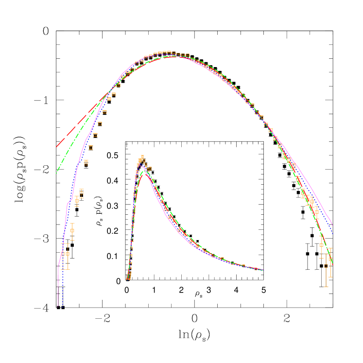
Figure 1 shows the redshift space PDF of the dark matter in spheres of radius $8h^{-1}{\rm Mpc}$. The main panel shows this using a $\log$-$\ln$ scale to emphasize the behaviour of the low probability tails, and the inset shows the same data using linear axes to highlight the behaviour near the peak of the distribution. Filled and open squares show the measurements in the simulation (i.e., before and after compressing the fingers-of-god). These indicate that fingers-of-god are most important in the denser cells; this is not unexpected, since dense cells host the most massive halos which have the largest virial motions.

Our perturbation theory based prediction is represented by the dotted (blue) curve — notice that it provides a significantly better fit to the simulations when the fingers-of-god have been compressed. The solid (magenta) curve is the perturbation theory based prediction with $B=0$ in equation (9), which corresponds to using our ellipsoidal collapse model but ignoring the effect on the variance associated with differences from a spherical shape. The dotted curve ($B=0.0486$) is always closer to the measurements than is the solid one ($B=0$), consistent with the real-space results presented in Lam & Sheth (2008)), although the difference between the two curves is not large. In what follows, we only show results for the case when $B=0.0486$. The dot-dashed (green) curve shows the Lognormal (equation 13) and the long-dashed (red) curve shows equation (14). Our model provides a better fit than these other more empirical curves, except in the highest density tail.

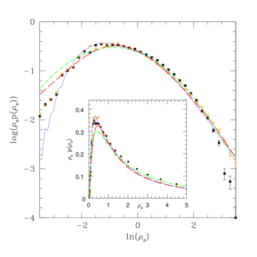
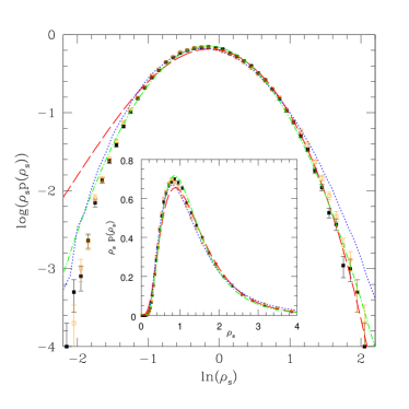
Figure 2 shows similar results for spheres of radius 4$h^{-1}{\rm Mpc}$ and 16$h^{-1}{\rm Mpc}$. In the larger cells, fingers-of-god are irrelevant, and the Lognormal provides a slightly better description than does our model, which again overshoots at large densities. The approach which assumes a simple mapping from real to redshift space overdensity fairs reasonably well at large densities, but underestimates the height of the peak of the distribution, and overestimates the PDF at lower densities. Our model is substantially better than the other two in the smaller 4$h^{-1}{\rm Mpc}$ cells.

4 Reconstruction of the initial distributions

In Lam & Sheth (2008) we described how the spherical collapse model could be used as the basis of a method for reconstructing the shape of the initial PDF from the Eulerian one. In principle, the method can be used as a consistency check for Gaussian initial conditions. We showed that, in real space, it can reconstruct the Gaussian form of the initial distribution from the highly skewed nonlinear PDF on scales where the rms fluctuation is about $2$ or less.

Extending this reconstruction method to redshift space is complicated by the fact that we know the spherical model is inadequate (it does not reproduce the Kaiser factor). However, the ellipsoidal collapse model, which we have shown works quite well, has many more parameters — the lengths and orientations of the three principal axes — so that the final density is determined by a stochastic rather than deterministic mapping.

So we have tried a simpler approach which is based on the fact that equation (14) provides a reasonable description of the redshift space PDF. Namely, we assume that

$$\delta_{s}=\delta_{r}\,(\sigma_{s}/\sigma_{r}),$$ (15)

and use the (square root of the) Kaiser factor in place of $\sigma_{s}/\sigma_{r}$; we have found that using our ellipsoidal collapse calculation of this quantity instead produces slightly worse results. Then we set

$$\nu\equiv\frac{1-[(1+\delta_{\rm s}\,\sigma_{r}/\sigma_{s})/N_{\rm sc}]^{-1/\delta_{\rm c}}}{\sigma_{\rm L}(M/N_{\rm sc})/\delta_{\rm c}},$$ (16)

where $\delta_{\rm c}$ is the critical linear density associated with collapse in the spherical model, and $N_{\rm sc}$ is the normalization factor (the analogue of equation 11) in the spherical model calculation of the real space PDF. Finally, we make a histogram of $\nu$ by weighting each cell which contributes to $p(\delta_{s})$ by its value of $(1+\delta_{s}\sigma_{r}/\sigma_{s})/N_{\rm sc}$.

Before showing how well this works, Figure 3 shows a test of our assumption that equation (15) is accurate, meaning that $\delta_{s}$ is linearly related to $\delta_{r}$, with little scatter around the mean relation. Evidently, these assumptions are reasonable on large scales (bottom and middle panels), but become increasingly worse on smaller scales (top).

Figure 3: Comparsion of real- and redshift-space overdensities in cells of radius $4h^{-1}$Mpc (top), $8h^{-1}$Mpc (middle) and $16h^{-1}$Mpc (bottom). Filled and open symbols are before and after fingers of god have been removed. They show the mean, and error bars show the rms, for narrow bins in $(\delta/\sigma)_{r}$. If equation (15) is accurate, then $(\delta/\sigma)_{s}-(\delta/\sigma)_{r}=0$ with little scatter.

Figure 4: Comparsion of the reconstructed linear PDF of $\delta/\sigma$ (histogram) with the expected zero-mean unit-rms Gaussian form (solid curve). Upper panels show results of reconstruction for $4h^{-1}{\rm Mpc}$ scale, middle panels show results for $8h^{-1}{\rm Mpc}$. lower panels show results for $16h^{-1}{\rm Mpc}$. Left- and right-hand panels show results of reconstructions which begin from the filled and open squares in the previous Figures (i.e. estimates of $p(\delta_{s})$ with and without fingers-of-god). Dotted curves in each panel show the corresponding nonlinear PDFs (equation 8).

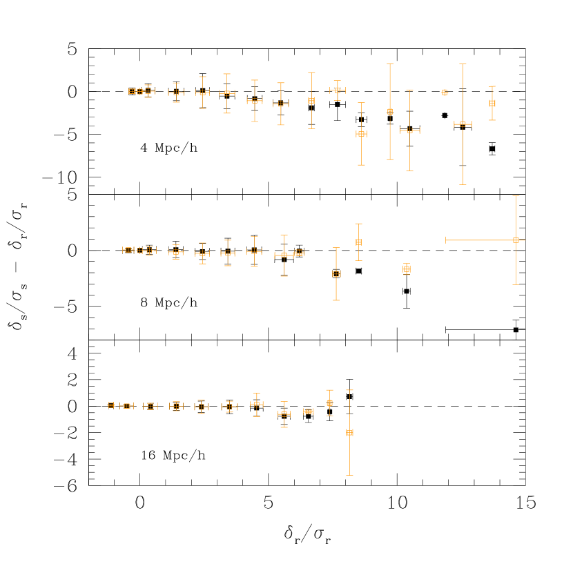
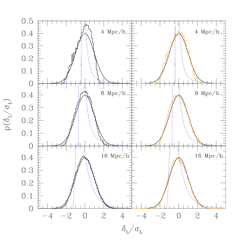
Figure 4 shows the reconstruction results for $4$, $8$ and $16h^{-1}{\rm Mpc}$ spheres. The left- and right-hand panels show the result of transforming the PDFs shown by filled and open squares in the previous Figures (i.e., full and compressed fingers of god). Smooth solid curves show a Gaussian distribution for comparison. The reconstruction method works well for the $8$ and $16h^{-1}{\rm Mpc}$ scales. This method even works for the smaller $4h^{-1}{\rm Mpc}$ scales if the fingers-of-god have been removed. The dotted curves show the corresponding nonlinear distributions (equation 8) to demonstrate that our reconstruction method transforms significantly skewed distributions back to the original symmetric gaussian shape.

5 Discussion

We have extended our previous work on the real space dark matter PDF to redshift space. To do so, we provided a simple parametrization of the evolution of the nonlinear density in the ellipsoidal collapse model. This shows explicitly how the model extends both the spherical collapse model, and the Zeldovich approximation (equations 26 and 7). This parametrization, with our prescription for relating spatial statistics in the initial and evolved fields (equation 8), results in excellent agreement with measurements from a numerical simulation, in both real (Figure 5) and redshift space (Figures 1 and 2). Our parametrization fares significantly better than analyses which are based on exact second and third order perturbative expansions of the ellipsoidal collapse evolution — these produce PDFs with a power-law tail at high densities which is a signature that the analysis is breaking down — a similar tail was seen for the Zeldovich approximation (Hui et al., 2000). Our approach also fares better than the Lognormal model, and one which assumes that redshift space overdensities are linearly proportional to those in real-space: $\delta_{s}=(\sigma_{s}/\sigma_{r})\,\delta_{r}$ where the constant of proportionality is given by the (square-root of the) ratio of the variances. The latter is known to be a good approximation on large scales — we find that it is accurate on small scales, except in underdense regions.

We also used our results to motivate a method for reconstructing the shape of the initial PDF from the nonlinear evolved redshift space PDF. This method works well on scales where the rms fluctuation is less than 2 when fingers-of-god have been removed (Figure 4). We are in the process of applying this method to reconstruct the baryonic ascoustic oscillation (BAO) peak in the correlation function (Eisenstein et al., 2007). Instead of using equation (16) it is also possible to formulate the reconstruction using equations (26) or (7); this is also the subject of work in progress.

While this provides a nice graphic reconstruction of the Gaussianity of the initial conditions, more work is necessary before it can be used to distinguish between a truly Gaussian model and the very mildly non-Gaussian models which are not yet excluded by the CMB (Komatsu et al., 2008). In this respect, it may be interesting to extend our method for estimating the nonlinear PDF to the family of non-Gaussian models which are currently studied in the context of using cluster abundances and clustering to constrain primordial non-Gaussianity (Slosar et al., 2008; Dalal et al., 2008; Lo Verde et al., 2008).

Appendix A Relation between initial and final density in the ellipsoidal collapse model

In this Appendix we derive relatively simple analytic approximations to the evolution of the density within a triaxial perturbation. The exact evolution of the perturbation is assumed to be described by the ellipsoidal collapse model of Bond & Myers (1996). Shen et al. (2006) provide a simple but useful approximation to this evolution which is based on a beautiful analysis of the collapsing ellipsoid problem by White & Silk (1979). It is this approximate solution which we exploit.

A.1 The collapse model

Gravity evolves the initial axes $(R_{1}^{i},R_{2}^{i},R_{3}^{i})$ of a triaxial object to $(R_{1},R_{2},R_{3})$ because

$$\frac{{\rm d}^{2}R_{k}}{{\rm d}t^{2}}=H_{0}^{2}\Omega_{\Lambda}R_{k}-4\pi G\bar{\rho}R_{k}\,\left(\frac{1+\delta}{3}+\frac{b_{k}^{\prime}}{2}\delta+\lambda^{\prime}_{{\rm ext,}k}\right),$$ (17)

where the interior and exterior tidal forces are respectively,

$$b^{\prime}_{k}(t)= \left(\prod_{i=1}^{3}R_{i}(t)\right)\int_{0}^{\infty}\frac{{\rm d}\tau}{[R_{k}^{2}(t)+\tau]\prod_{j=1}^{3}[R_{j}^{2}(t)+\tau]^{1/2}}$$

$$-\frac{2}{3},$$ (18)

$$\lambda^{\prime}_{{\rm ext,}k}(t)= \frac{D(t)}{D(t_{i})}\left[\lambda_{k}(t_{i})-\frac{\delta_{i}}{3}\right]$$ (19)

(Bond & Myers, 1996). Here $\lambda_{k}$ are the initial eigenvalues of the deformation tensor, and the initial conditions of equation (17) are set by the Zeldovich Approximation:

$$R_{k}(t_{i}) =a_{i}[1-\lambda_{k}(t_{i})],$$ (20)

$$\frac{{\rm d}R_{k}(t_{i})}{{\rm d}t} =H(t_{i})R_{k}(t_{i})-a(t_{i})H(t_{i})f_{1}\lambda(t_{i}),$$ (21)

where $f_{1}={\rm d}\ln D/{\rm d}\ln a$ and $D(t)$ is the linear growth factor.

Although equation (17) in general must be solved numerically, Shen et al. (2006) showed that the following approximation was rather accurate:

$$\begin{split}R_{k}(t)=&\frac{a(t)}{a_{i}}R_{k}(t_{i})[1-D(t)\lambda_{k}]\\ &-\frac{a(t)}{a_{i}}R_{h}(t_{i})\left[1-\frac{D(t)}{3}\delta_{i}-\frac{a_{e}(t)}{a(t)}\right],\end{split}$$ (22)

where $R_{h}(t_{i})=3/\sum_{j}R_{j}(t_{i})^{-1}$ and $a_{e}(t)$ is the expansion factor of a spherical universe with initial overdensity $\delta_{i}=\sum_{j}\lambda_{j}(t_{i})$. This expression is inspired by an analysis of collapsing ellipsoids by White & Silk (1979). The first term in the expression above is the Zeldovich Approximation to the evolution; the second term is a correction to this approximation. When $\lambda_{2}=\delta_{i}/3$ then the evolution of the second axis is almost exactly like that of a sphere with initial overdensity $\delta_{i}$.

A.2 Evolution to a spherical volume

For an Eulerian sphere of $R_{\rm E}$, equation (22) implies that

$$R_{1}^{i}[1-D(t)\lambda_{1}]=R_{2}^{i}[1-D(t)\lambda_{2}]=R_{3}^{i}[1-D(t)\lambda_{3}].$$ (23)

Substitute into the definition of $R_{h}(t_{i})$

$$R_{h}(t_{i})=\frac{3}{\sum_{j}R_{j}(t_{i})^{-1}}=\frac{R_{k}(t_{i})(1-D(t)\lambda_{k})}{1-D(t)\delta_{i}/3},$$ (24)

where $k=1,2,3$. Therefore we can write the evolved $R_{k}(t)$ as

$$\frac{R_{\rm E}}{R_{k}^{i}}=\frac{a_{e}(t)/a(t)}{1-D(t)\delta_{i}/3}[1-D(t)\lambda_{k}],$$ (25)

where $R_{k}^{i}=R_{k}(t_{i})$. This writes the evolution as that in the Zeldovich Approximation, times a correction factor which is simply the ratio of the evolved and initial radii of a Zeldovich sphere $(1-D\delta_{i}/3)$ divided by the same ratio in the exact spherical evolution model. Thus, the evolved overdensity is

$$\rho =1+\delta=\prod_{j=1}^{3}\frac{R_{j}^{i}}{R_{\rm E}}\approx\frac{(1-D(t)\delta_{i}/3)^{3}}{(a_{e}(t)/a(t))^{3}}\,\prod_{j=1}^{3}\frac{1}{1-D(t)\lambda_{j}}$$

$$\approx\frac{(1-D(t)\delta_{i}/3)^{3}}{(1-D(t)\delta_{i}/\delta_{c})^{\delta_{c}}}\,\prod_{j=1}^{3}\frac{1}{1-D(t)\lambda_{j}}.$$ (26)

The final expression uses a simple approximation for the evolution in the spherical collapse model:

$$\frac{a(t)}{a_{e}(t)}\approx\left(1-D(t)\frac{\delta_{i}}{\delta_{c}}\right)^{-\delta_{c}/3}$$ (27)

(Bernardeau, 1994; Sheth, 1998), where $\delta_{c}\approx 5/3$. Notice that when all the eigenvalues are identical, then equation (26) reduces to the spherical collapse model.

Figure 5: The real space non-linear PDF. Symbols show measurements in a numerical simulation (from Lam & Sheth 2008). The solid (blue) curve uses our approximation to ellipsoidal collapse (equation 26) and the dashed (red) curve is based on our approximation to spherical collapse (equation 27).

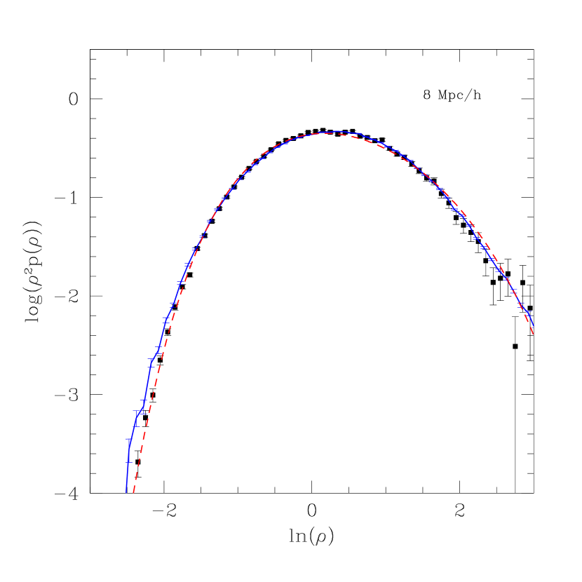
Insertion of equation (27) or (26) into equation (8) of the main text yields models for the redshift-space PDF associated with spherical and ellipsoidal collapse, respectively. The corresponding models for the real-space PDF are given by setting $f=0$ in that expression. These real-space models are shown by the dashed (red) or solid (blue) curves; both are in excellent agreement with the measured real-space PDF (symbols).

A.3 Evolution to an arbitrary shape

When the Eulerian volume in consideration is triaxial, the computation of the overdensity is less trivial. In general one must solve a system of non-linear equations for $x_{k}\equiv a(t)R_{k}^{i}/a_{i}R_{k}(t)$ in

$$\begin{split}x_{k}[1-&D(t)\lambda_{k}]=\\ &1+3\left(1-\frac{D(t)\delta_{i}}{3}-\frac{a_{e}(t)}{a(t)}\right)\left(\sum_{j=1}^{3}\frac{R_{k}}{R_{j}}\frac{1}{x_{j}}\right)^{-1}.\end{split}$$ (28)

The overdensity is $1+\delta=\prod_{j=1}^{3}x_{j}$. The above equation can be solved numerically or iteratively with

$$x_{k}^{(n+1)}= \left[1+3\left(1-\frac{D(t)\delta_{i}}{3}-\frac{a_{e}(t)}{a(t)}\right)\left(\sum_{j=1}^{3}\frac{R_{k}}{R_{j}}\frac{1}{x_{j}^{(n)}}\right)^{-1}\right]$$

$$\times[1-D(t)\lambda_{k}]^{-1}$$ (29)

$$x_{k}^{(0)}= \frac{1-D(t)\delta_{i}/3}{a_{e}(t)/a(t)}\frac{1}{1-D(t)\lambda_{k}}.$$ (30)

An analytical expression for the overdensity of the ellipsoid can be obtained if we make the approximation that the collapse of the second axis is very close to that in the spherical model. Shen et al. (2006) show why this is almost always an excellent approximation. One can then approximate the collapse of the second axis using either of the two expressions below:

$$\frac{R_{2}^{i}}{R_{2}(t)}\approx\left\{\begin{aligned} &\frac{1-D(t)\delta_{i}/3}{a_{e}(t)/a(t)}\frac{1}{1-D(t)\lambda_{2}},\\ &\left(1-\frac{D(t)\delta_{i}}{\delta_{c}}\right)^{-\delta_{c}/3}.\end{aligned}\right.$$ (31)

The first expression is our approximate description of evolution to an Eulerian sphere, and the second is simply the spherical collapse model.

Substituting these approximations into equation (22) yields

$$\frac{R_{k}^{i}}{R_{2}}[1-D(t)\lambda_{k}]=\left\{\begin{aligned} &\frac{R_{k}}{R_{2}}-1+\frac{1-D(t)\delta_{i}/3}{a_{e}(t)/a(t)},\\ &\frac{R_{k}}{R_{2}}-1+\frac{1-D(t)\lambda_{2}}{a_{e}(t)/a(t)},\end{aligned}\right.$$ (32)

for which the associated overdensities are

$$\begin{split}\rho=&\prod_{j=1}^{3}\frac{R_{j}^{i}}{R_{j}}\\ =&\left\{\begin{aligned} &\prod_{j=1}^{3}\frac{a(t)}{a_{e}(t)}\frac{1-D(t)\delta_{i}/3}{1-D(t)\lambda_{j}}\left(\frac{R_{2}}{R_{j}}+\frac{a_{e}(t)}{a(t)}\frac{1-R_{2}/R_{j}}{1-D(t)\delta_{i}/3}\right),\\ &\prod_{j=1}^{3}\frac{a(t)}{a_{e}(t)}\frac{1-D(t)\lambda_{2}}{1-D(t)\lambda_{j}}\left(\frac{R_{2}}{R_{j}}+\frac{a_{e}(t)}{a(t)}\frac{1-R_{2}/R_{j}}{1-D(t)\lambda_{2}}\right),\end{aligned}\right.\end{split}$$ (33)

where $a_{e}(t)$ is approximated by equation (27). Compared to equation (26) the last term in the first approximation is the extra factor accounting for the non-spherical shape in the final volume. For $R_{1}=R_{2}=R_{3}$, this extra factor is unity and equation (33) has the same expression as in the spherical case.

Appendix B Perturbative treatment of redshift space distortions

Kaiser (1987) derives a simple relation between the real and redshift space power spectra. Fisher (1995) provides a very different derivation of Kaiser’s expression. The Zeldovich approximation provides yet another derivation of this relation (Ohta et al., 2004). We show that our approximation for ellipsoidal collapse also reproduces this expression, and then use it to derive the next order corrections. This analysis is useful because Scoccimarro (2004) has shown that Kaiser’s approximation is accurate only on rather large scales.

Before we present the algebra, it is worth noting that the approximation used in the main text for the real space evolution of a collapsing ellipsoid follows from (i) writing the full ellipsoidal collapse as the Zeldovich approximation times a correction factor which is the ratio of the evolution of a sphere in the Zeldovich approximation to that in the spherical collapse model; and (ii) using our convenient approximation to the exact evolution in the spherical collapse model. In the perturbative analysis which follows, we have chosen notation which illustrates what happens if we keep approximation (i), but treat the spherical collapse model exactly rather than approximately.

We begin by writing the relation between the linear and nonlinear overdensities in the spherical evolution model as

$$1+\delta\equiv\left(\frac{a(t)}{a_{e}(t)}\right)^{3}=1+\sum_{n=1}^{\infty}\frac{\nu_{n}}{n!}\,\delta_{l}^{n}.$$ (34)

Then the exact result has

$$\nu_{2} =\frac{2}{3}\left(2-\frac{g_{2}}{g_{1}^{2}}\right)$$

$$\nu_{3} =\frac{2}{9}\left(10-12\frac{g_{2}}{g_{1}^{2}}+\frac{g_{3a}}{g_{1}^{3}}+6\frac{g_{3b}}{g_{1}^{3}}\right),$$ (35)

where $g_{i}$ is the $i$th order growth factor (e.g. Fosalba & Gaztañaga 1998). For $\Lambda\neq 0$ $(g_{2}/g_{1}^{2})\approx-(3/7)\,\Omega^{-1/143}$, $(g_{3a}/g_{1}^{3})\approx-(1/3)\,\Omega^{-4/275}$ and $(g_{3b}/g_{1}^{3})\approx(10/21)\,\Omega^{-269/17875}$ Bouchet et al. (1995). The dependence on $\Omega$ is so weak that we can use the $\Omega=1$ values to find $\nu_{2}\approx 1.62$ and $\nu_{3}\approx 3.926$. In contrast, our previous approximation has

$$\nu_{n}\approx\prod_{i=0}^{n-1}\frac{\delta_{\rm c}+i}{\delta_{\rm c}}$$ (36)

so $\nu_{2}\approx 1.6$ and $\nu_{3}\approx 3.52$.

With this notation, our approximation for the evolution of an ellipsoid is

$$1+\delta_{r} =\left(1-\frac{\delta_{l}}{3}\right)^{3}\left(1+\sum_{n=1}^{\infty}\frac{\nu_{n}}{n!}\delta_{l}^{n}\right)\prod_{k=1}^{3}(1-\lambda_{k})^{-1}$$

$$=1+\grave{\delta_{r}}^{(1)}+\grave{\delta_{r}}^{(2)}+\grave{\delta_{r}}^{(3)}+\dots,$$ (37)

where

$$\grave{\delta_{r}}^{(1)}= \sum_{j=1}^{3}\lambda_{j}$$

$$\grave{\delta_{r}}^{(2)}= \frac{\nu_{2}}{2}\,\delta_{l}^{2}+\frac{\delta_{l}^{2}}{3}-\sum_{j\neq k}\lambda_{j}\lambda_{k}$$

$$\grave{\delta_{r}}^{(3)}= \frac{\nu_{3}}{6}\,\delta_{l}^{3}+\frac{17}{27}\,\delta_{l}^{3}-2\delta_{l}\,\sum_{j\neq k}\lambda_{j}\lambda_{k}+\lambda_{1}\lambda_{2}\lambda_{3}.$$ (38)

In each expression above, the first terms are those associated with the spherical model, and the others are the corrections which come from the ellipsoidal collapse. The terms associated with a perturbation theory analysis of the exact ellipsoidal collapse model are given by Ohta et al. (2004). The expressions above show the terms which are associated with our simple approximation to the exact evolution. They differ slightly from those associated with the exact analysis; e.g., the second order expression associated with the exact analysis is $(4/17)(\delta_{l}^{2}-3I_{2})$, but they otherwise have the same form, suggesting that our simple expression captures the essence of the ellipsoidal collapse evolution.

The overdensity in redshift space is

$$1+\delta_{s}\equiv \frac{1+\delta_{r}}{1-\sum_{k=1}^{3}\grave{g}_{k}^{z}\,e_{k}^{2}}$$

$$= 1+\grave{\delta}_{s}^{(1)}+\grave{\delta}_{s}^{(2)}+\grave{\delta}_{s}^{(3)}+\dots,$$ (39)

where

$$\grave{g}^{z}_{k}= \frac{\left\{R_{k}^{i}\lambda_{k}-A_{h}^{i}\,\left[f_{1}\delta_{l}-\left(1+\sum_{n=1}^{\infty}\frac{\nu_{n}}{n!}\delta_{l}^{n}\right)^{-4/3}\left(\sum_{m=1}^{\infty}f_{m}\frac{\nu_{m}}{m!}\delta_{l}^{m}\right)\right]/3\right\}}{R_{k}^{i}(1-\lambda_{k})-A_{h}^{i}[1-\delta_{l}/3-(1+\sum_{n=1}^{\infty}\frac{\nu_{n}}{n!}\delta_{l}^{n})^{-1/3}]}$$

$$= f_{1}\lambda_{k}+\frac{1}{3}(\frac{\nu_{2}}{2}f_{2}-\frac{4}{3}f_{1})\delta_{l}^{2}+f_{1}\lambda_{k}^{2}$$

$$+\frac{\delta_{l}^{2}}{3}\left[(\frac{\nu_{2}}{2}f_{2}-\frac{4}{3}f_{1})\lambda_{k}+(\frac{\nu_{3}}{6}f_{3}-\frac{2\nu_{2}}{3}f_{1}-\frac{5\nu_{2}}{6}f_{2}+2f_{1})\delta_{l}\right]$$

$$+\frac{1}{3}(\frac{\nu_{2}}{2}f_{2}-\frac{4}{3}f_{1})\lambda_{k}\delta_{l}^{2}+f_{1}\lambda_{k}\left[\lambda_{k}^{2}+\delta_{l}^{2}(\frac{\nu_{2}}{6}-\frac{2}{9})\right]+\dots,$$ (40)

and $f_{i}={\rm d}\ln g_{i}/{\rm d}a$. Thus,

$$\delta_{s}^{(1)}= \delta_{r}^{(1)}+\Delta_{z}^{(1)}$$

$$\delta_{s}^{(2)}= \delta_{r}^{(2)}+\Delta_{z}^{(2)}+\delta_{r}^{(1)}\,\Delta_{z}^{(1)}$$

$$\delta_{s}^{(3)}= \delta_{r}^{(3)}+\Delta_{z}^{(3)}+\delta_{r}^{(2)}\,\Delta_{z}^{(1)}+\delta_{r}^{(1)}\,\Delta_{z}^{(2)},$$ (41)

and

$$\Delta_{z}^{(1)}= f_{1}\sum_{k=1}^{3}\lambda_{k}\,e_{k}^{2}$$

$$\Delta_{z}^{(2)}= f_{1}\sum_{k=1}^{3}\left[\frac{\nu_{2}}{2}\,\frac{f_{2}}{f_{1}}-\frac{4}{3}\right]\frac{\delta_{l}^{2}}{3}\,e_{k}^{2}$$

$$+f_{1}^{2}\,\sum_{k=1}^{3}\lambda_{k}^{2}\,e_{k}^{2}+f_{1}^{2}\sum_{j,k=1}^{3}\lambda_{j}\lambda_{k}\,e_{j}^{2}e_{k}^{2}$$

$$\Delta_{z}^{(3)}= f_{1}\sum_{k=1}^{3}\frac{\delta_{l}^{2}}{3}\left[(\frac{\nu_{2}}{2}\,\frac{f_{2}}{f_{1}}-\frac{4}{3})\,\lambda_{k}+(\frac{\nu_{3}}{6}\,\frac{f_{3}}{f_{1}}-\frac{2\nu_{2}}{3}-\frac{5\nu_{2}}{6}\,\frac{f_{2}}{f_{1}}+2)\,\delta_{l}\right]e_{k}^{2}$$

$$+2f_{1}^{2}\sum_{j,k=1}^{3}\,\lambda_{j}\,\left[(\frac{\nu_{2}}{2}\,\frac{f_{2}}{f_{1}}-\frac{4}{3})\,\frac{\delta_{l}^{2}}{3}+\lambda_{k}^{2}\right]\,e_{j}^{2}e_{k}^{2}$$

$$+f_{1}^{3}\sum_{i,j,k=1}^{3}\lambda_{i}\lambda_{j}\lambda_{k}\,e_{i}^{2}e_{j}^{2}e_{k}^{2}.$$ (42)

Our leading order term, $\delta_{s}^{(1)}$ is the same as that of Ohta et al. (2004), who showed that $\sigma_{s}^{2}\equiv\langle(\delta_{s}^{(1)})^{2}\rangle$, where the angle brackets denote the result of averaging over the Euler angles as well as the distribution of the $\lambda_{i}$, leads to Kaiser’s formula. The logic which leads to our second order term is consistent with that of Watts & Taylor (2001), except that because our collapse model considers motions relative to the center of the object, it has no term which accounts for the motion of the center of mass. There are additional small differences which arise from the fact that our description of ellipsoidal collapse is based on our approximate model - had we computed our perturbation series expansion using the exact collapse model, we would have reproduced their expressions.

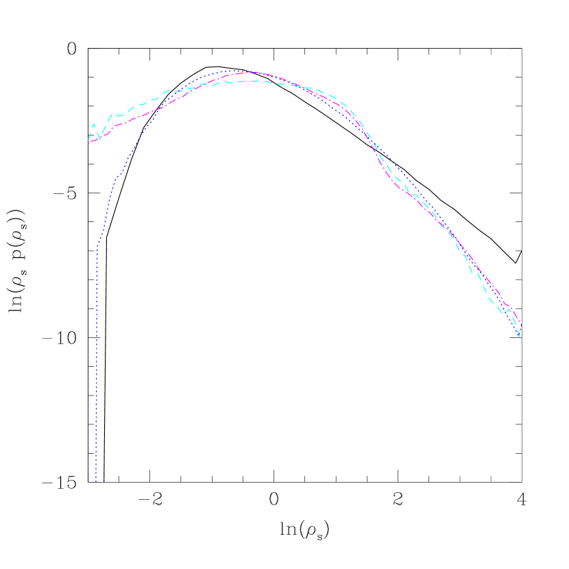
Figure 6 illustrates one reason why we have used our approximation for the nonlinear dynamics, rather than worked with exact perturbative expansions to higher and higher orders. The dotted line shows the redshift space PDF associated with our approximation; the main text shows that it provides an good description of the simulations. The solid line shows the result of using the Zeldovich approximation for the evolution, and setting $\sigma=\sigma(\bar{\rho}V)$ whatever the shape and overdensity of the initial object Hui et al. (2000). This results in a PDF with a tail that scales as $\rho_{s}^{-3}$ at high densities — a signature that the approach has broken down. The dashed curve shows the result of using equation (9) for $\sigma$ instead. This helps somewhat — although the onset of the $\rho_{s}^{-3}$ tail is shifted to larger $\rho_{s}$, the shape of the PDF in underdense regions is adversely affected. The dot-dashed curve shows the result of going to third-order in the exact ellipsoidal collapse model (recall that, in this context, the Zeldovich approximation is like the first order term). This modifies the shape of the PDF slightly, but the problem at small $\rho_{s}$ remains.

Figure 6: Four approximations to the redshift space PDF. Solid line shows the prediction associated with the Zeldovich approximation, but assuming that the associated $\sigma$ is the same for all cells of volume $V$ (Hui et al. 2000). Dashed and dot-dashed curves show the first- and third-order exact ellipsoidal collapse based analyses; these do account for the fact that $\sigma$ depends on the Lagrangian size and shape (e.g. Ohta et al. 2004). Dotted curve shows the PDF associated with our approximation to the exact evolution.

References

- Barrow & Silk (1981) Barrow J. D., Silk J., 1981, Astrophys. J., 250, 432
- Bernardeau (1994) Bernardeau F., 1994, Astron. Astrophys., 291, 697
- Bernardeau et al. (2002) Bernardeau F., Colombi S., Gaztañaga E., Scoccimarro R., 2002, Phys. Rep., 367, 1
- Betancort-Rijo (1991) Betancort-Rijo J., 1991, Mon. Not. R. Astron. Soc., 251, 399
- Betancort-Rijo & López-Corredoira (2002) Betancort-Rijo J., López-Corredoira M., 2002, Astrophys. J., 566, 623
- Bond & Myers (1996) Bond J. R., Myers S. T., 1996, Astrophys. J. Supp., 103, 1
- Bouchet et al. (1995) Bouchet F. R., Colombi S., Hivon E., Juszkiewicz R., 1995, Astron. Astrophys., 296, 575
- Dalal et al. (2008) Dalal N., White M., Bond J. R., Shirokov A., 2008, ArXiv e-prints, astro-ph/0803.3453
- Desjacques (2008) Desjacques V., 2008, Mon. Not. R. Astron. Soc., pp 727–+
- Desjacques & Smith (2008) Desjacques V., Smith R. E., 2008, ArXiv e-prints, astro-ph/0805.2145
- Doroshkevich (1970) Doroshkevich A. G., 1970, Astrofizika, 6, 581
- Eisenstein et al. (2007) Eisenstein D. J., Seo H.-J., Sirko E., Spergel D. N., 2007, Astrophys. J., 664, 675
- Fisher (1995) Fisher K. B., 1995, Astrophys. J., 448, 494
- Fosalba & Gaztañaga (1998) Fosalba P., Gaztañaga E., 1998, Mon. Not. R. Astron. Soc., 301, 503
- Gaztañaga & Croft (1999) Gaztañaga E., Croft R. A. C., 1999, Mon. Not. R. Astron. Soc., 309, 885
- Hivon et al. (1995) Hivon E., Bouchet F. R., Colombi S., Juszkiewicz R., 1995, Astron. Astrophys., 298, 643
- Hui et al. (2000) Hui L., Kofman L., Shandarin S. F., 2000, Astrophys. J., 537, 12
- Icke (1973) Icke V., 1973, Astron. Astrophys., 27, 1
- Jackson (1972) Jackson J. C., 1972, Mon. Not. R. Astron. Soc., 156, 1P
- Kaiser (1987) Kaiser N., 1987, Mon. Not. R. Astron. Soc., 227, 1
- Kofman et al. (1994) Kofman L., Bertschinger E., Gelb J. M., Nusser A., Dekel A., 1994, Astrophys. J., 420, 44
- Komatsu et al. (2008) Komatsu E., Dunkley J., Nolta M. R., Bennett C. L., Gold B., Hinshaw G., Jarosik N., Larson D., Limon M., Page L., Spergel D. N., Halpern M., Hill R. S., Kogut A., Meyer S. S., Tucker G. S., Weiland J. L., Wollack E., Wright E. L., 2008, ArXiv e-prints, astro-ph/0803.0547
- Lam & Sheth (2008) Lam T. Y., Sheth R. K., 2008, Mon. Not. R. Astron. Soc., 386, 407
- Lin et al. (1965) Lin C. C., Mestel L., Shu F. H., 1965, Astrophys. J., 142, 1431
- Lo Verde et al. (2008) Lo Verde M., Miller A., Shandera S., Verde L., 2008, Journal of Cosmology and Astro-Particle Physics, 4, 14
- Ohta et al. (2004) Ohta Y., Kayo I., Taruya A., 2004, Astrophys. J., 608, 647
- Padmanabhan & Subramanian (1993) Padmanabhan T., Subramanian K., 1993, Astrophys. J., 410, 482
- Protogeros & Scherrer (1997) Protogeros Z. A. M., Scherrer R. J., 1997, Mon. Not. R. Astron. Soc., 284, 425
- Scherrer & Gaztañaga (2001) Scherrer R. J., Gaztañaga E., 2001, Mon. Not. R. Astron. Soc., 328, 257
- Scoccimarro (2004) Scoccimarro R., 2004, Phys. Rev. D, 70, 083007
- Scoccimarro & Frieman (1999) Scoccimarro R., Frieman J. A., 1999, Astrophys. J., 520, 35
- Shen et al. (2006) Shen J., Abel T., Mo H. J., Sheth R. K., 2006, Astrophys. J., 645, 783
- Sheth (1998) Sheth R. K., 1998, Mon. Not. R. Astron. Soc., 300, 1057
- Sheth et al. (2001) Sheth R. K., Mo H. J., Tormen G., 2001, Mon. Not. R. Astron. Soc., 323, 1
- Slosar et al. (2008) Slosar A., Hirata C., Seljak U., Ho S., Padmanabhan N., 2008, ArXiv e-prints, astro-ph/0805.3580
- Smith et al. (2003) Smith R. E., Peacock J. A., Jenkins A., White S. D. M., Frenk C. S., Pearce F. R., Thomas P. A., Efstathiou G., Couchman H. M. P., 2003, Mon. Not. R. Astron. Soc., 341, 1311
- Smith et al. (2007) Smith R. E., Sheth R. K., Scoccimarro R., 2007, ArXiv e-prints, astro-ph/0712.0017
- Watts & Taylor (2001) Watts P. I. R., Taylor A. N., 2001, Mon. Not. R. Astron. Soc., 320, 139
- White & Silk (1979) White S. D. M., Silk J., 1979, Astrophys. J., 231, 1
- Zel’Dovich (1970) Zel’Dovich Y. B., 1970, Astron. Astrophys., 5, 84