The Letter Q (and Quantitative Constraints on the QGP)

Abstract

In this proceedings, we briefly review the methodology from [1] for quantitatively constraining theoretical model parameters from experimental measurements including statistical and systematic uncertainties. We extend this methodology to additional parton energy-loss calculations for single inclusive high $p_{T}$ particle suppression, and also extend the comparisons to di-jet observations. This is only the start of a process to give quantitative constraints on the quark-gluon plasma, and substantial theoretical uncertainties need to be reduced/resolved in a parallel path.

1 Introduction

The field of relativistic heavy ion physics is undergoing a necessary transition from a field focused on the declaration of discovery - of thermalized partonic matter or the quark-gluon plasma, to one focused on the quantitative understanding of the unique properties of the medium created. This effort requires a more sophisticated and full treatment of experimental uncertainties, in particular systematic uncertainties and their underlying correlations. Additionally, the effort requires the reconciliation of variant theoretical approaches, or the discarding of some in favor of others. This proceedings focuses primarily on the first effort, though with some commentary on the second.

2 Single Hadron High $p_{T}$ Suppression

Fig. 1.: (Color Online) The left panel shows the PHENIX $\pi^{0}$ nuclear modification factor as a function of $p_{T}$. The curves are different calculations of the AMY+Hydro model corresponding to different input $\alpha_{s}$ values. The right panel shows the correlation between the input $\alpha_{s}$ coupling and the predicted nuclear modification factor.

Fig. 2.: (Color Online) The modified $\chi^{2}$ distribution as a function of the AMY+Hydro model input parameter $\alpha_{s}$.

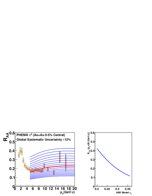
High $p_{T}$ $\pi^{0}$’s are suppressed in heavy ion reactions [2], as shown in the left panel of Fig. 1. The experimental uncertainties are separated into three categories. Type A uncertainties are point-to-point uncorrelated and are shown as standard error lines. For this measurement, they are dominated by statistical uncertainties. Type B uncertainties are point-to-point correlated and are shown as grey bars. They are dominated by the energy scale uncertainty in the Electro-magnetic calorimeters and have some contribution for $p_{T}\approx 15-20$ GeV/c from photon shower merging effects. Type C uncertainties are globally correlated (i.e. all points move by a common multiplicative factor). Note that this does not mean that all points move up and down together on a linear y-axis plot. This contribution is quoted as a $\pm$ 12% global systematic uncertainty and has roughly equal contributions from the uncertainty in the nuclear  thickness function $T_{AA}$ (as determined by a Glauber model) and from the proton-proton inelastic cross section absolute normalization. It is notable that these last two sources of uncertainty may prove quite difficult to reduce in the future.

These Type B and C uncertainties correspond to one RMS deviations about the measured value. In the analysis that follows, these uncertainties are assumed to follow a Gaussian distribution with the corresponding RMS value. It is notable that if there are many contributions to the uncertainties, the Central Limit Theorem makes this assumption more solid. However, if the best fit results are a few standard deviations away in the systematic uncertainties, one should view the exact numerical fit result with some skepticism. Of course, if this is the case, the best fit typically is a very poor fit. It is also notable that if systematic uncertainties are quoted as ’full extent’, then they cannot be added in quadrature and preserve their ’full extent’ nature.

Every publication of data in the field on which a full quantitative analysis is to be performed needs to explicitly quote these RMS uncertainty contributions in their appropriately labeled category.

The methodology is detailed in [1], and here we just summarize the key result. One calculates a modified $\chi^{2}$ for a given data set with points ($y_{i}$) and a given theoretical model with predictions $\mu_{i}$ as a function of parameter set $p$. One includes the possibility of systematic offsets given by the number of standard deviations for Type B ($\epsilon_{b}$) and for Type C ($\epsilon_{c}$):

$$\tilde{\chi}^{2}={\left[\sum_{i=1}^{n}{{(y_{i}+\epsilon_{b}\sigma_{b_{i}}+\epsilon_{c}y_{i}\sigma_{c}-\mu_{i}(\vec{p}))^{2}}\over{{\tilde{\sigma}}_{i}^{2}}}+{\epsilon_{b}^{2}}+{\epsilon_{c}^{2}}\right]}\qquad,$$ (1)

where ${\tilde{\sigma}}_{i}$ is the uncertainty scaled by the multiplicative shift in $y_{i}$ such that the fractional error is unchanged under shifts

$$\tilde{\sigma}_{i}=\sigma_{i}\left(\frac{y_{i}+\epsilon_{b}\sigma_{b_{i}}+\epsilon_{c}y_{i}\sigma_{c}}{y_{i}}\right)\qquad.$$ (2)

Fundamentally one is determining if the penalty for moving the data by some number of standard deviations in a systematic uncertainty is compensated by an overall reduction in the modified $\chi^{2}$ due to an improved statistical fit.

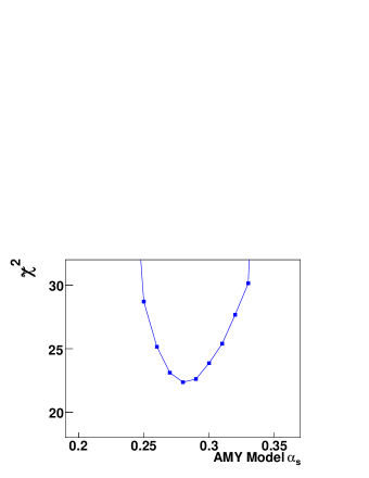
An example comparison with a theoretical model is shown in Fig. 1. In this case, the $\mu_{i}$ are the AMY+Hydro theoretical calculations [3] as a function of the input parameters $p$, specifically being the coupling $\alpha_{s}$. In [3], the authors utilize the AMY formalism for parton energy-loss and simulate the underlying medium with a hydrodynamic evolution model. The authors assert that “once temperature evolution is fixed by the initial conditions and evolution [by 3+1 dimensional hydrodynamics], the coupling $\alpha_{s}$ is the only quantity which is not uniquely determined.” Shown in the left panel of Fig. 1 are calculations from this model for different input values of $\alpha_{s}$. The left panel shows how the nuclear modification factor at $p_{T}=20$ GeV/c varies as a function of this input coupling value. We have then applied the full constraint method and show the modified $\chi^{2}$ as a function of $\alpha_{s}$ in Fig. 2.

Model	Constrained Medium Parameters	p-value
PQM	$\langle$q̂$\rangle$ = 13.2 ${}^{+2.1}_{-3.2}$ [1 stdev] and ${}^{+6.3}_{-5.2}$ [2 stdev]  GeV2/fm	9.0%
GLV	$(dN/dy)_{gluon}=1400^{+270}_{-150}$ [1 stdev] and ${}^{+510}_{-290}$ [2 stdev]	5.5%
WHDG	$(dN/dy)_{gluon}=1400^{+200}_{-375}$ [1 stdev] and ${}^{+600}_{-540}$ [2 stdev]	1.3%
ZOWW	$\epsilon_{0}=1.9^{+0.2}_{-0.5}$ [1 stdev] and ${}^{+0.7}_{-0.6}$ [2 stdev]  GeV/fm	7.8%
AMY+Hydro	$\alpha_{s}=0.280^{+0.016}_{-0.012}$ [1 stdev] and ${}^{+0.034}_{-0.024}$ [2 stdev]	5.0%
Linear	b (intercept) = $0.168^{+0.033}_{-0.032}$ [1 stdev] and ${}^{+0.065}_{-0.066}$ [2 stdev]	11.6%
	m (slope) = $0.0017^{+0.0035}_{-0.0039}$ [1 stdev] and ${}^{+0.0070}_{-0.0076}$ [2 stdev] ($c$/GeV)

Table 1.: Quantitative constraints on the medium parameters from various energy-loss models.

The resulting constraint for the AMY + Hydro model and for a variety of parton energy-loss calculations and a linear functional fit are given in Table 1. It is critical to note that each constraint is assuming a perfect model calculation with only one unknown parameter, i.e. the uncertainty is from experimental sources only.

Fig. 3.: (Color Online) For the PQM energy-loss model, the correlation between the $\langle$q̂$\rangle$and the nuclear modification factor is shown. The left panel is a linear-linear display, and the right panel is a log-log display.

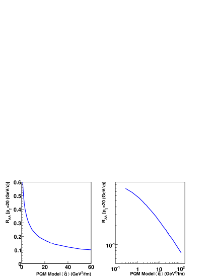
There are a number of general observations that can be made at this point. In all of these calculations, there is a clear minimum in the modified $\chi^{2}$ and a reasonably well defined one- and two-standard deviation limit. In [4], the authors refer to the “fragility of high $p_{T}$ hadron spectra as a hard probe.” The usage of this term “fragility” is ambiguous in the literature. Some simply refer to it with respect to the fact that as one increases the color-charge density or medium transport value $\langle$q̂$\rangle$, the nuclear modification factor $R_{AA}$ appears to saturate. Thus, one can speculate that for some large value (for example $\langle$q̂$\rangle$$>5$ GeV²/fm), the uncertainty in determining $R_{AA}$ gets very large. However, viewing such trends on a linear y-axis scale can be quite deceptive. Shown in Fig. 3 are predictions from the Parton Quenching Model (PQM) [5] for different $\langle$q̂$\rangle$values. In the right panel, shown on a log x-axis and log y-axis scale, is the modification factor versus $\langle$q̂$\rangle$. It is striking that it appears linear on this plot for $\langle$q̂$\rangle$$>5$. Thus, for a given fractional uncertainty in measuring $R_{AA}$, one always gets the same fractional uncertainty on $\langle$q̂$\rangle$. Very similar results are obtained with other model calculations.

If this is not the meaning of “fragility” (in a purely statistical constraint sense), others refer to it in reference to the concept of surface emission bias. Imagine a beam of partons aimed at the corona of a dense medium. No measurement of the emitted particles provides information about the core of the medium (since the partons are not aimed there). However, if one had a model of the density distribution of the medium, then measuring (for example) the color-charge density of the corona, one can (via this distribution) learn about the density in the core. However, this knowledge is “fragile” in the sense that it depends more and more sensitively on the knowledge of the medium density distribution. It is interesting that in the paper discussing this “fragility” issue [4], the authors employ a very unrealistic uniform cylindrical geometry, such that the density in the corona is identical to the density in the core. It is also notable that this geometry gets the distribution of hard scattering positions incorrect as well.

3 Di-Jet Observables

Fig. 4.: (Color Online) The left panel shows the STAR dijet for per trigger away-side integrated yield ($D_{dAu/AuAu}$) as a function of $z_{T}$ from d-Au and Au-Au. The right panel is the ratio ($I_{AA}$). An additional 5% and 7% Type C uncertainty is including in the $D_{dAu/AuAu}$ and $I_{AA}$ results, respectively [8]. Also shown are the ZOWW theory calculations for different input energy-loss parameter ($\epsilon_{0}$) values.

Fig. 5.: (Color Online) The modified $\chi^{2}$ for the ZOWW calculations for the $I_{AuAu}$ results (red line), the $D_{AuAu}$ only (blue line), and the $D_{AuAu}$ including the theoretical scale uncertainty (magenta line).

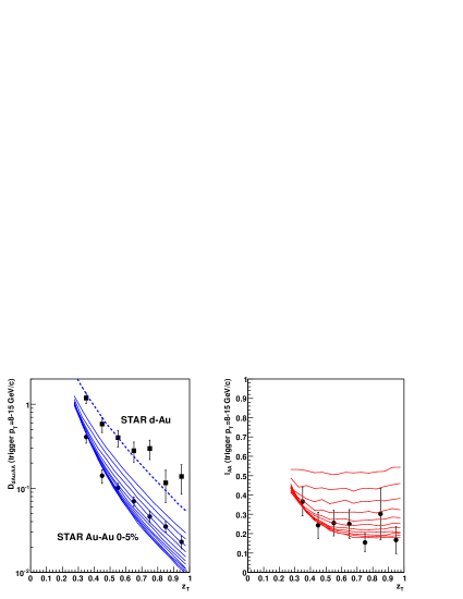
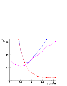
Regardless of the definition of “fragility”, it is always wise to search for additional discriminating experimentally accessible observables. In [6], they speculate that di-jet observables will be more sensitive to medium parameters. In the context of their calculation (ZOWW), they show that $I_{AA}$ (the modification of per trigger away-side yields) has a steeper dependence on their energy-loss parameter $\epsilon_{0}$ (GeV/fm), than the single inclusive modification factor $R_{AA}$. Thus, if one had identical experimental uncertainties on the two quantities, then $I_{AA}$ would provide the stricter constraint.

Shown in Fig. 4 are the experimental data from the STAR experiment [7], and the calculations from the ZOWW model [6]. If we apply a 7% Type C uncertainty to the STAR $I_{AA}$ results [8], the resulting constraint is $\epsilon_{0}=2.9^{+???}_{-0.6}$ [one std. dev.] and ${}^{+???}_{-0.9}$ [two std. dev.]. The ’???’ refers to the fact that within the parameter ranges available, there is no upper constraint. This is notably worse than the constraint from $R_{AA}$ given in Table 1. In fact, the two results do not overlap each other within the one standard deviation uncertainties. The worse constraint from $I_{AA}$ is due to the poor statistics in the $d-Au$ reference (used instead of proton-proton) for the modification factor. This will be remedied in the near future with the much larger $d-Au$ data set taken in 2007-2008.

It is notable that in [6], they show a rather tight $\epsilon_{0}$ constraint in a figure labeled $I_{AA}$. However, the actual constraint was derived from just comparing the Au-Au result alone ($D_{AuAu}$). Thus, the constraint is only derived from the Au-Au data in the left panel of Fig. 4. The resulting modified $\chi^{2}$’s from $I_{AA}$ and $D_{AuAu}$ alone are shown in Fig. 5. It is notable that the fit to the $D_{AuAu}$ alone is a rather poor fit, which can be visually seen in Fig. 4 where the shape of the data points for $z_{T}>0.4$ do not match any of the theory curves. If one only fits $D_{AuAu}$, there is a definite additional theory uncertainty from the pQCD scale uncertainty in the NLO calculation (shown in [6]). If this is included, the constraint is much looser, again shown in Fig. 5. Future high statistics data sets will allow for a more detailed study. Also, the use of the variable $z_{T}$ may hide many details, and an optimal high statistics presentation should first include fine binning in trigger $p_{T}$ for $I_{AuAu}$.

4 Summary

We summarize with a set of observations. On the experimental side, we have a well understood method for inclusion of statistical and systematic uncertainties. Experiments need to carefully quantify these Type A, B, and C uncertainties for all relevant measurements. It will be very interesting to see if larger p-p and d-Au data sets reconcile the $R_{AA}$ and $I_{AA}$ constraints.

On the theoretical side, one needs to resolve fundamental disconnects about whether perturbative calculations with modest $\alpha_{s}$ fully describe parton energy loss. Currently the PQM results [5] indicate that the perturbative calculations fail. In either case, this must be reconciled at the appropriate scales with the picture of the bulk medium being strongly coupled (near-perfect fluid) and not being describable in a perturbative framework. Also, all calculations must include realistic geometries, fluctuations, and running of the coupling (if possible) so that the discussions and comparisons can focus on the more fundamental physics questions.

References

- [1] A. Adare, et al, arXiv:0801.1665 [nucl-ex], (to be published)
- [2] A. Adare, et al, arXiv:0801.4020v1 [nucl-ex], (to be published)
- [3] G-Y Qin, et al, Phys. Rev. Lett. 100, 072301 (2008).
- [4] K.J. Eskola, H. Honkanen, C.A. Salgado, U.A. Wiedemann, Nucl. Phys. A747, 511 (2005).
- [5] A. Dainese, C. Loizides, G. Paic, Eur. Phys. J C38, 461 (2005). C. Loizides, Eur. Phys. J. C49, 339 (2007).
- [6] H. Zhang, J.F. Owens, E. Wang, X-N Wang, Phys. Rev. Lett. 98: 212301 (2007).
- [7] J. Adams, et al, Phys. Rev. Lett. 97, 162301 (2006).
- [8] P. Jacobs, Private Communication.