Entropy estimates of small data sets

Abstract

Estimating entropies from limited data series is known to be a non-trivial task. Naïve estimations are plagued with both systematic (bias) and statistical errors. Here, we present a new “balanced estimator” for entropy functionals (Shannon, Rényi and Tsallis) specially devised to provide a compromise between low bias and small statistical errors, for short data series. This new estimator out-performs other currently available ones when the data sets are small and the probabilities of the possible outputs of the random variable are not close to zero. Otherwise, other well-known estimators remain a better choice. The potential range of applicability of this estimator is quite broad specially for biological and digital data series.

Journal Reference: J. Phys. A: Math. Theor. 41 (2008) 202001.

1 Introduction

In statistical mechanics and information theory, entropy is a functional that measures the information content of a statistical ensemble or equivalently the uncertainty of a random variable. Its applications in physics, biology, computer science, linguistic, etc are countless. For example, it has become a key tool in data mining tasks arising from high-throughput biological analyses.

Historically, the most important example of such a functional is the Shannon (or information) entropy [1, 2]. For a discrete random variable $x$, which can take a finite number, $M$, of possible values $x_{i}\in\left\{x_{1},\ldots,x_{M}\right\}$ with corresponding probabilities $p_{i}\in\left\{p_{1},\ldots,p_{M}\right\}$, this entropy is defined by:

$$\begin{array}[]{rl}H_{S}=&-\displaystyle\sum_{i=1}^{M}p_{i}\textnormal{ln}(p_{i}).\end{array}$$ (1)

Recently, various generalizations, inspired by the study of $q$-deformed algebras and special functions, have been investigated, most notably the Rényi entropy [3]:

$$\begin{array}[]{rl}H_{R}(q)=&\dfrac{1}{1-q}\textnormal{ln}\left(\displaystyle\sum_{i=1}^{M}p^{q}_{i}\right),\end{array}$$ (2)

with $p\geq 0$, which, in particular, reduces to the Shannon entropy in the limit $q\rightarrow 1$. Also, the Tsallis entropy [4]:

$$\begin{array}[]{rl}H_{T}(q)=&\dfrac{1}{q-1}\left(1-\displaystyle\sum_{i=1}^{M}p^{q}_{i}\right),\end{array}$$ (3)

although controversial, has generated a large burst of research activity.

In general, the full probability distribution for a given stochastic problem is not known and, in particular, in many situations only small data sets from which to infer entropies are available. For example, it could be of interest to determine the Shannon entropy of a given DNA sequence. In such a case, one could estimate the probability of each element $i$ to occur, $p_{i}$, by making some assumption on the probability distribution, as for example (i) parametrizing it [5], (ii) dropping the most unlikely values [6] or (iii) assuming some a priori shape for the probability distribution [7, 8]. However, the easiest and most objective way to estimate them is just by counting how often the value $x_{i}$ appears in the data set [9, 10, 11, 12, 14, 15, 16]. Denoting this number by $n_{i}$ and dividing by the total size of the data set one obtains the relative frequency:

$$\begin{array}[]{rl}\hat{p}_{i}=&\dfrac{n_{i}}{N}\end{array}$$ (4)

which naïvely approximates the probability $p_{i}$. Obviously, the entropy of the data set can be approximated by simply replacing the probabilities $p_{i}$ by $\hat{p}_{i}$ in the entropy functional. For example, the Shannon entropy can be estimated by:

$$\begin{array}[]{rl}H_{S}\approx\hat{H}_{S}^{naive}=&-\displaystyle\sum_{i=1}^{M}\hat{p}_{i}\textnormal{ln}(\hat{p}_{i})=-\displaystyle\sum_{i=1}^{M}\dfrac{n_{i}}{N}\textnormal{ln}\left(\dfrac{n_{i}}{N}\right).\end{array}$$ (5)

The quantity $\hat{H}_{S}^{naive}$ is an example of an estimator of the entropy, in a very similar sense as $\hat{p}_{i}$ is an estimator of $p_{i}$. However, there is an important difference stemming from the non-linear nature of the entropy functional. The frequencies $\hat{p}_{i}$ are unbiased estimators of the probabilities, i.e., their expectation value $\langle\hat{p}_{i}\rangle$ (where $\langle\cdot\rangle$ stands for ensemble averages) coincides with the true value of the estimated quantity:

$$\begin{array}[]{rl}\langle\hat{p}_{i}\rangle=&\dfrac{\langle n_{i}\rangle}{N}=p_{i}.\end{array}$$ (6)

In other words, the frequencies $\hat{p}_{i}$ approximate the probabilities $p_{i}$ with certain statistical error (variance) but without any systematic error (bias). Contrarily, naïve entropy estimators, such as $\hat{H}_{S}^{naive}$, in which the $p_{i}$ are simply replaced by $n_{i}/N$ are always biased, i.e. they deviate from the true value of the entropy not only statistically but also systematically. Actually, defining an error variable $\epsilon_{i}=(\hat{p_{i}}-p_{i})/p_{i}$, and replacing $p_{i}$ in Eq.(1) by its value in terms of $\epsilon_{i}$ and $\hat{p_{i}}$, it is straightforward to verify that the bias, up to leading order, is $-\frac{M-1}{2N}$, which is a significant error for small $N$ and vanishes only as $N\rightarrow\infty$ [12]. A similar bias, owing in general to the nonlinearity of the entropy functional, appears also for the Rényi and Tsallis entropies.

Therefore, the question arises whether it is possible to find improved estimators which reduce either the bias or the variance of the estimate. More generally, the problem can be formulated as follows. Given an arbitrary entropy functional of the form:

$$\begin{array}[]{rl}H=&F\left[\displaystyle\sum_{i=1}^{M}h(p_{i})\right]\end{array}$$ (7)

(where $F$ is a generic function) we want to find an estimator

$$\begin{array}[]{rl}\hat{H}=&F\left[\displaystyle\sum_{i=1}^{M}\chi_{n_{i}}\right]\end{array}$$ (8)

such that the bias

$$\begin{array}[]{rl}\Delta=&\langle\hat{H}\rangle-H\end{array}$$ (9)

or the mean squared deviation (the statistical error)

$$\begin{array}[]{rl}\sigma^{2}=&\left\langle\left(\hat{H}-\langle\hat{H}\rangle\right)^{2}\right\rangle\end{array}$$ (10)

or a combination of both are as small as possible. At the very end of such a calculation the estimator is defined by $N+1$ real numbers $\chi_{n_{i}}$ [13], which depend on the sample size $N$. For example, the naïve estimator for the Shannon entropy would be given in terms of

$$\begin{array}[]{rl}\chi_{n_{i}}^{naive}\;=&-\dfrac{n_{i}}{N}\textnormal{ln}\left(\dfrac{n_{i}}{N}\right).\end{array}$$ (11)

The search for improved estimators has a long history. To the best of our knowledge, the first to address this question was Miller in 1955 [14], who suggested a correction to reduce the bias of the estimate of Shannon entropy, given by:

$$\begin{array}[]{rl}\chi_{n_{i}}^{Miller}\;=&-\dfrac{n_{i}}{N}\textnormal{ln}\left(\dfrac{n_{i}}{N}\right)+\dfrac{1}{2N}.\end{array}$$ (12)

The correction exactly compensates the leading order of the bias, as reported above. In this case the remaining bias vanishes as $1/N^{2}$ as $N\rightarrow\infty$. This result was improved by Harris in 1975 [15], who calculated the next-leading order correction. However, his estimator depends explicitly on the (unknown) probabilities $p_{i}$, so that its practical importance is limited.

In another pioneering paper, Grassberger, elaborating upon previous work by Herzel [16], proposed an estimator which provides further improvement and gives a very good compromise between bias and statistical error [9]. For the Shannon entropy his estimator is given by

$$\chi_{n_{i}}^{Grassberger}=\dfrac{n_{i}}{N}\left(\ln N-\psi(n_{i})-\frac{\left(-1\right)^{n_{i}}}{n_{i}(n_{i}+1)}\right),$$ (13)

where $\psi(x)$ is the derivative of the logarithm of the Gamma function, valid for all $i$ with $n_{i}>0$. According to [9], the function $\psi(x)$ can be approximated by

$$\psi(n_{i})\approx\ln x-\frac{1}{2x}$$ (14)

for large $x$, giving

$$\begin{array}[]{rl}\chi_{n_{i}}^{Grassberger}\approx&-\dfrac{n_{i}}{N}\textnormal{ln}\left(\dfrac{n_{i}}{N}\right)+\dfrac{1}{2N}-\dfrac{\left(-1\right)^{n_{i}}}{N(n_{i}+1)}\end{array}$$ (15)

This method can be generalized to $q$-deformed entropies.

More recently, a further improvement for the Shannon case has been suggested by Grassberger [10]

$$\chi_{n_{i}}^{GS}=\dfrac{n_{i}}{N}\left[\psi(N)-\psi(n_{i})-(-1)^{n_{i}}\int_{0}^{1}\frac{t^{n_{i}-1}}{1+t}dt\right].$$ (16)

This estimator can be recast (see Eqs. (28),(29),(35) of Ref. [10]) as

$$\chi_{n_{i}}^{GS}=\frac{n_{i}}{N}\Bigl{(}\ln N-G_{n_{i}}\Bigr{)}\,,$$ (17)

where the $G_{n}$ satisfy the recurrence relation

$$G_{1} = -\gamma-\ln 2$$ (18)

$$G_{2} = 2-\gamma-\ln 2$$ (19)

$$G_{2n+1} = G_{2n}$$ (20)

$$G_{2n+2} = G_{2n}+2/(2n+1)$$ (21)

with $\gamma=-\psi(1)$. This estimator constitutes the state of the art for Shannon entropies, but unfortunately, it cannot be straightforwardly extended to more general q-deformed entropy functionals, for which [9] remains the best available option. These results were further generalized by Schürmann [11] with different balances between statistical and systematic errors.

It should be emphasized that an ideal estimator does not exist, instead the choice of the estimator depends on the structure of data to be analyzed [17]. For example, the above discussed estimators [9, 10] work satisfactorily if the probabilities $p_{i}$ are sufficiently small. This is the case in many applications of statistical physics, where the number of possible states, $M$, in an ensemble is usually extremely large so that the probability $p_{i}$ for an individual state $i$ is very small. On the other hand, this assumption does not always hold for empirical data sets such as digital data streams and DNA sequences.

The performance of the estimators worsens as the values of $p_{i}$ get larger. This is due to the following reason: the numbers $n_{i}$, which count how often the value $x_{i}$ appears in the data set, are generically distributed as binomials, i.e. the probability $P_{n_{i}}$ to find the value $n_{i}$ is given by:

$$\begin{array}[]{rl}P_{n_{i}}({p_{i}})=&\dbinom{N}{n_{i}}p_{i}^{n_{i}}(1-p_{i})^{N-n_{i}}\end{array}$$ (22)

where $\dbinom{N}{n_{i}}=\dfrac{N!}{n_{i}!(N-n_{i})!}$ are binomial coefficients. For $p_{i}\ll 1$ this can be approximated by a Poisson distribution, which is the basis for the derivation of Eq. (13). For large values $p_{i}$, however, this assumption is no longer justified and this results in large fluctuations (even if the bias remains small).

It is important to note that it is not possible to design an estimator that minimizes both the bias and the variance to arbitrarily small values. The existing studies have shown that there is always a delicate tradeoff between the two types of errors. For example, minimizing the bias usually comes at the expense of the variance, which increases significantly. Moreover, it can be proved that neither the variance nor the bias can be reduced to zero for finite $N$ [18]. Therefore, it is necessary to study estimators with different balances between systematic and statistical errors, as it was done e.g. in the work by Schürmann [11].

In the present work we introduce two estimators, which can be used to measure any of the entropy functionals discussed above. Both of them are specifically designed for short data series where the probabilities $p_{i}$ take (in general) non-small values. The first one reduces the bias as much as possible at the expense of the variance, and is mostly of academic interest and discussed only for illustration purposes. The second one seeks for a robust compromise between minimizing bias and variance together, is very easy to implement numerically, and has a broad potential range of applicability. The estimator itself can be improved by adapting various of its elements to each specific problem.

2 Low-bias estimator

The starting point is the observation that the entropy $H$ and its estimators $\hat{H}$ in Eq. (7) and Eq. (8) involve sums over all possible values of the data set. Therefore, as the bias can be minimized by minimizing the errors of each summand, the problem can be reduced to minimize

$$\begin{array}[]{rl}\delta(p_{i})=&\langle\chi_{n_{i}}\rangle-h(p_{i})=\left(\displaystyle\sum_{n_{i}=0}^{N}P_{n_{i}}(p_{i})\chi_{n_{i}}\right)-h(p_{i})\end{array}$$ (23)

over a broad range of $p_{i}$ as much as possible.

A theorem by Paninski [18] states that it is impossible to reduce the bias to zero for all $p_{i}\in[0,1]$ since an estimator is always a finite polynomial in $p_{i}$ while the true entropy is usually not a polynomial. However, it is possible to let the bias vanish at $N+1$ points $p_{i}$ in the interval $[0,1]$ because the determination of the different $\chi_{n_{i}}$ requires $N+1$ independent equations.

For the sake of illustration, let us choose here equidistant points $p_{j}=j/N$, with $j=0,1,\ldots,N$. In general, other choices, more appropriate to each specific case, should be employed. The resulting set of linear equations reads:

$$\begin{array}[]{rl}\delta(j/N)=0\Longrightarrow&\displaystyle\sum_{n_{i}=0}^{N}P_{n_{i}}(j/N)\chi_{n_{i}}=h(j/N),\hskip 56.9055ptj=0,1,\ldots,N.\end{array}$$ (24)

Figure 1: Fluctuations, $\sigma^{2}$, as defined by Eq. (10), for three different Shannon entropy estimates (the naïve one, the improved estimator introduced in [10], and the low-bias estimator defined in this paper) for a binary sequence ($M=2$) of length $N=20$. Inset: Bias, $\Delta$, as defined by Eq. (9), for the low-bias estimator showing the N+1 vanishing points with amplitude oscillations.

Introducing the notation $h_{j}=h(j/N)$ and $P_{j,n_{i}}=P_{n_{i}}(j/N)$ this last expression takes the form:

$$\begin{array}[]{rl}\displaystyle\sum_{n_{i}=0}^{N}P_{j,n_{i}}\chi_{n_{i}}=&h_{j},\hskip 56.9055ptj=0,1,\ldots,N\end{array}$$ (25)

or, in short, ${\bf P}\overrightarrow{\chi}=\overrightarrow{h}$, where ${\bf P}$ is the so-called multinomial matrix [19]. To find the solution $\overrightarrow{\chi}={\bf P}^{-1}\overrightarrow{h}$, the matrix:

$$\begin{array}[]{rl}P_{j,n_{i}}=&\dbinom{N}{n_{i}}p_{j}^{n_{i}}(1-p_{j})^{N-n_{i}}=\dbinom{N}{n_{i}}\left(\dfrac{j}{N}\right)^{n_{i}}\left(1-\dfrac{j}{N}\right)^{N-n_{i}},\end{array}$$ (26)

whose elements are binomial distributions, has to be inverted. For small $N$ this inversion is most easily done numerically. However, we were also able to invert the matrix analytically, leading us to the closed form [20]:

$$\begin{array}[]{cc}\hat{P}_{i,j}^{-1}=&\displaystyle\sum_{k=0}^{N}\sum_{l=0}^{N}\dbinom{i}{k}\dbinom{l}{j}\dfrac{N^{k}k!(N-k)!}{N!}\dfrac{(-1)^{l+j}}{l!}s(l,k)\end{array}$$ (27)

where $s(l,k)$ denotes the Stirling numbers of the first kind [21]. Having inverted the matrix, the numbers $\chi_{n_{i}}$ determining the estimators can be computed for any given entropy functional by a simple matrix multiplication.

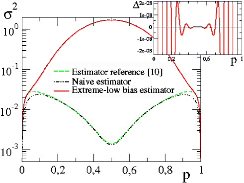
Figure 1 illustrates a comparison for the Shannon case between the low-bias estimator and other well-known ones for the simple example of a binary sequence of $N=20$ bits $x=0,1$ (i.e. $M=2$), where the value $1$ appears with probability $p$ and $0$ with probability $1-p$. The bias of the low-bias estimator vanishes exactly only at values of $p$ multiples of $1/20$, and takes small values in between (see inset of Fig.1). On the other hand, the fluctuations for both the naïve estimator and the one in [10] remain bounded, while they diverge for the low-bias case (Fig.1 ). This unbounded growing of statistical fluctuations makes the low-bias estimator useless for practical purposes.

3 Balanced Estimator

Aiming at solving the previously illustrated problem with uncontrolled statistical fluctuations, in this section we introduce a new balanced estimator designed to minimize simultaneously both the bias and the variance over a wide range of probabilities. This is of relevance for analyzing small data sets where statistical fluctuations are typically large and a compromise with minimizing the bias is required.

As before, ignoring correlations between the $n_{i}$ both bias and statistical errors can be optimized by minimizing the errors of the summands in their corresponding expressions. Therefore, the problem can be reduced to minimize the bias for each state

$$\begin{array}[]{rl}\delta(p_{i})=&\langle\chi_{n_{i}}\rangle-h(p_{i})\end{array}$$ (28)

and the variance within such a state

$$\begin{array}[]{rl}\sigma^{2}(p_{i})=&\left\langle\left(\chi_{n_{i}}-\langle\chi_{n_{i}}\rangle\right)^{2}\right\rangle\end{array}$$ (29)

over a broad range of $p_{i}\in[0,1]$, where $n_{i}\in{0,1,\ldots,N}$ is binomially distributed. Since we are interested in a balanced compromise error, it is natural to minimize the squared sum:

$$\Phi^{2}(p_{i})=\delta^{2}(p_{i})+\sigma^{2}(p_{i}).$$ (30)

This quantity measures the total error for a particular value of $p_{i}$. Therefore, the average error over the whole range of $p_{i}\in[0,1]$ is given by:

$$\begin{array}[]{rl}\overline{\Phi^{2}_{i}}=&\displaystyle\int^{1}_{0}dp_{i}w(p_{i})\Phi^{2}(p_{i})\end{array}$$ (31)

where $w(p_{i})$ is a suitable weight function that should be determined for each specific problem.

We discuss explicitly here the simplest case $w(p_{i})\equiv 1$ (obviously, any extra knowledge of the probability values should lead to a non-trivial distribution of weights, resulting in improved results). Inserting Eq. (28) and Eq. (29) into Eq. (31), the average error is given by:

$$\begin{array}[]{rl}\overline{\Phi^{2}_{i}}=&\displaystyle\int^{1}_{0}dp_{i}\left[\left(\displaystyle\sum_{n_{i}=0}^{N}P_{n_{i}}(p_{i})\chi_{n_{i}}^{2}\right)+h^{2}(p_{i})-2h(p_{i})\left(\displaystyle\sum_{n_{i}=0}^{N}P_{n_{i}}(p_{i})\chi_{n_{i}}\right)\right].\end{array}$$ (32)

Now, we want to determine the numbers $\chi_{n_{i}}$ in such a way that the error given by Eq.32 is minimized. Before proceeding, let us make it clear that instead of minimizing the mean-square error for each of the possible states ($i=1,...,M$) one could also minimize the total mean-square error defined using Eq.(9) and (10) rather than Eq. (28) and (29) to take into account correlations between boxes which, in general, will improve the final result. For example, for binary sequences this can be easily done, and leads to the same result as reported on what follows [20].

As a necessary condition, the partial derivatives:

$$\begin{array}[]{rl}\dfrac{\partial}{\partial\chi_{n_{i}}}\overline{\Phi^{2}_{i}}=&0\end{array}$$ (33)

have to vanish, i.e.:

$$\begin{array}[]{rl}2\displaystyle\int^{1}_{0}dp_{i}P_{n_{i}}(p_{i})\left[\chi_{n_{i}}-h(p_{i})\right]=&0\end{array}$$ (34)

for all $n_{i}=0,1,\ldots,N$. Therefore, the balanced estimator is defined by the numbers:

$$\begin{array}[]{rl}\chi_{n_{i}}^{bal}=&\dfrac{\displaystyle\int^{1}_{0}dp_{i}P_{n_{i}}(p_{i})h(p_{i})}{\displaystyle\int^{1}_{0}dp_{i}P_{n_{i}}(p_{i})}=(N+1)\displaystyle\int^{1}_{0}dp_{i}P_{n_{i}}(p_{i})h(p_{i}).\end{array}$$ (35)

where we have explicitly integrated over $p_{i}$ the binomial distribution.

In the Shannon case, where $h(p_{i})=-p_{i}\textnormal{ln}(p_{i})$, the integration can be explicitely carried out, leading to [22]:

$$\begin{array}[]{rl}\chi_{n_{i}}=&\dfrac{n_{i}+1}{N+2}\displaystyle\sum_{j=n_{i}+2}^{N+2}\dfrac{1}{j}\end{array}$$ (36)

so that the final result for the balanced estimator of Shannon entropy is given by:

$$\begin{array}[]{rl}\hat{H}_{S}^{bal}=&\dfrac{1}{N+2}\displaystyle\sum_{i=1}^{M}\left[(n_{i}+1)\displaystyle\sum_{j=n_{i}+2}^{N+2}\dfrac{1}{j}\right].\end{array}$$ (37)

Similarly, it is possible to compute $\chi_{n{i}}$ for a power $h(p_{i})=p_{i}^{q}$, which is the basis for all $q$-deformed entropies:

$$\begin{array}[]{rl}\chi_{n_{i}}(q)=&\dfrac{\Gamma(N+2)\Gamma(n_{i}+1+q)}{\Gamma(N+2+q)\Gamma(n_{i}+1)}\end{array}$$ (38)

The balanced estimators for Rényi [23] and Tsallis entropy are then given respectively by:

$$\hat{H}_{R}^{bal}(q)=\dfrac{1}{1-q}\textnormal{ln}\left[\displaystyle\sum_{i=1}^{M}\chi_{n_{i}}(q)\right],~{}~{}$$ (39)

and

$$\hat{H}_{T}^{bal}(q)=\dfrac{1}{q-1}\left[1-\displaystyle\sum_{i=1}^{M}\chi_{n_{i}}(q)\right].$$ (40)

Figure 2: Mean squared error $\Phi^{2}=\langle\left(\hat{H}-H\right)^{2}\rangle$ of different entropy estimators (Upper row: Shannon (left); Rényi with $q=1.5$ (right); Lower row: Tsallis with $q=1.5$) for a binary sequence of $N=20$, as a function of $p$. The set of possible values is $\left\{x_{1}=1,x_{2}=0\right\}$ and the probabilities, $\left\{p_{1}=p,p_{2}=1-p\right\}$, respectively.

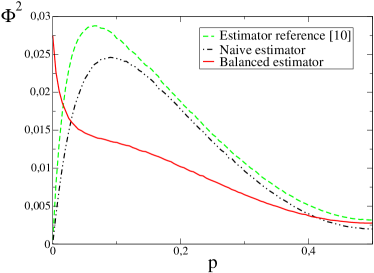
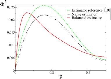
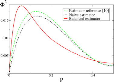
To illustrate the performance of these estimators, let us consider again a binary sequence of $N$ bits $x=0,1$ (i.e. $M=2$) occurring with probabilities $1-p$ and $p$ respectively. In Fig. 2 we plot the mean squared deviation $\Phi^{2}=\langle\left(\hat{H}-H\right)^{2}\rangle$ of various estimators from the true value of the Shannon as well as the Rényi entropy as a function of $p$. For such a short bit sequence, the performance of the Grassberger’s estimator using the parameter $\Phi^{2}$, is even worse than the naïve one. This is not surprising since Grassberger’s estimator is designed for small probabilities $p_{i}\ll 1$, while in the present example one of the probabilities $p$ or $1-p$ is always large and thus the estimator is affected by large fluctuations. The balanced estimator, however, reduces mean squared error considerably over an extended range of $p$ while for small $p$ and $0.4<p<0.6$ it fails. Similar plots can be obtained for the Tsallis entropy.

The advantage of the balanced estimator compared to standard ones decreases with increasing $N$. One of the reasons is the circumstance that the fluctuations of the estimator are basically determined by the randomness of the $n_{i}$ and, therefore, are difficult to reduce.

4 Conclusions

We have designed a new “balanced estimator” for different entropy functionals (Shannon, Rényi, and Tsallis) specially adequate for the analysis of small data sets where the possible states appear with not-too-small probabilities. To construct it, first we have illustrated a known result establishing that systematic errors (bias) and statistical errors cannot both be simultaneously reduced to arbitrarily small values when constructing an estimator for a limited data set. In particular, we have designed a low-bias estimator and highlighted that it leads to uncontrolled statistical fluctuations. This hinders the practical usefulness of such a low-bias estimator.

On the other hand, we have designed a new estimator that constitutes a good compromise between minimizing the bias and keeping controlled statistical fluctuations. We have illustrated how this balanced estimator outperforms (in reducing simultaneously bias and fluctuations) previously available ones in special situations the data sets are sufficiently small and the probabilities are not too small. Obviously situations such as in Fig. 2 are the ‘worst case’ for estimators like (13) and (16) which were designed to be efficient for large $M$. If any of these conditions is not fulfilled Grassberger’s and Schürmann’s estimator remains the best choice.

The balanced method fills a gap in the list of existing entropy estimators, is easy to implement for Shannon, Rényi and Tsallis entropy functional and therefore its potential range applicability is very large, specially in analyses of short biological (DNA, genes, etc.) data series.

The balanced estimator proposed here is simple but by no means ‘optimal’ for two reasons. First, we made no effort to optimize the location of the mesh points $p_{j}$, which for simplicity are assumed to be equidistant. Moreover, we did not optimize the weights $w(p_{j})$ towards a Bayesian estimate, as e.g. attempted by Wolpert and Wolf [8]. Further effort in this direction would be desirable.

We acknowledge financial support from the Spanish Ministerio de Educación y Ciencia (FIS2005-00791) and Junta de Andalucía (FQM-165).

References

- [1] C. E. Shannon, Bell Syst. Tech. J. 27, 379 (1948).
- [2] T.M. Cover and J.A. Thomas, Elements of Information Theory, John Wiley and Sons Ltd., Canada (2006).
- [3] A. Rényi, in Proceedings of the Berkeley Symposium on Mathematics, Statistics and Probability, 547 (1960). Rényi, Probability Theory, Amsterdam, North Holland (1970).
-
[4]
C. Tsallis, J. Stat. Phys. 52, 479 (1988);
see also http://tsallis.cat.cbpf.br/ biblio.htm. - [5] T. Pöschel, W. Ebeling and H. Rosé, J. Stat. Phys. 80, 1443 (1995).
[6]
W. Ebeling and G. Nicolis, Chaos,
Solitons and Fractals
2, 635 (1992);
H. Kantz and T. Schürmann, Chaos 6, 167 (1996);
T. Dudok de Wit, Eur. Phys. J. B 11, 513 (1999). -
[7]
D. Holste, H. Herzel and I. Grosse, ICCS Proceedings, 589 (1998);
D. Holste, I. Grosse and H. Herzel, J. Phys. A 31, 2551 (1998);
I. Nemenman, W. Bialek and R. R. R. van Steveninck, Phys. Rev. E 69, 056111 (2004). - [8] D. H. Wolpert and D. R. Wolf, Phys. Rev. E 52, 6841 (1995).
- [9] P. Grassberger, Phys. Letters A 128, 369 (1988), see corrections in [10].
- [10] P. Grassberger, eprint condmat/0307138, unpublished (2003).
- [11] T. Schürmann, J. Phys. A 37, L295 (2004).
- [12] M. S. Roulston, Physica D 125, 285 (1999),
- [13] This is so because the estimator depends only on , which can take possible values.
- [14] G. Miller, Information Theory in Psychology II-B, ed. H. Quastler, Glencoe, Illinois; Free Press, 95 (1955). See also, G. P. Basharin, Theory Prob. App. 4, 333 (1959).
- [15] B. Harris Topics on information Theory, 323 , ed. I. Csiszar, Amsterdam, North Holland (1975).
- [16] H. Herzel, Syst. Anal. Model Sim. 5, 435 (1988).
- [17] See, for instance, T. Schürmann and P. Grassberger, Chaos 6, 414 (1996).
- [18] L. Paninski, Neural Computation 15, 1191 (2003).
[19]
The matrix is well known for
biologists, as it is a common transition matrix in population
genetics. See,
R. G. Khazanie and H. E. McKean, Biometrika 53, 37 (1966);
R. A. Blythe and A. J. McKane, J. Stat. Mech., P07018 (2007). - [20] J. A. Bonachela, H. Hinrichsen, and M. A. Muñoz, Pre-print (2008). See also, D. S. Moak, Proc. Am. Math. Soc. 108, 1 (1990).
- [21] M. Abramowitz and I. Stegun, eds., Handbook of Mathematica Functions, Dover, New York, (1965).
- [22] The calculation requires using the definition of Harmonic numbers of first-order and binomial coefficients.
- [23] Here the influence of the non-linearity of the logarithm on statistical averages is neglected.