Further author information: L.H.K. E-mail: kauffman@uic.edu, S.J.L. Jr.: E-mail: lomonaco@umbc.edu
The Fibonacci Model and the Temperley-Lieb Algebra
Abstract
We give an elementary construction of the Fibonacci model, a unitary braid group representation that is universal for quantum computation. This paper is dedicated to Professor C. N. Yang, on his -th birthday.
keywords:
knots, links, braids, quantum computing, unitary transformation, Jones polynomial, Temperley-Lieb algebra1 Introduction
This paper gives an elementary construction for the unitary representation of the Artin braid group that constructs the well-known Fibonacci model. This model gives a topological basis for quantum computation. The present paper is an outgrowth of our papers [9, 10, 11] and is related to the analysis of the quantum algorithms for the Jones polynomial in the paper by Shor and Jordan [18]. We show that unitary representations of the braid group arise naturally in the context of the Temperely - Lieb algebra. The Fibonacci model is usually constructed by using recoupling theory. Here we show how the model emerges naturally from braid group representations to the Temperley-Lieb algebra. We use the idea of recoupling and change of basis in process spaces to motivate the construction, but we do not have to rely on any machinery of recoupling theory. This makes the present paper self-contained.
For the reader interested in the relevant background in topological quantum computing we recommend the following references { [20, 2, 3, 4, 5, 6, 14, 16, 17, 19, 1, 15] }.
Here is a very condensed presentation of how unitary representations of the braid group are constructed via topological quantum field theoretic methods. For simplicity assmue that one has a single (mathematical) particle with label that can interact with itself to produce either itself labeled or itself with the null label When interacts with the result is always When interacts with the result is always One considers process spaces where a row of particles labeled can successively interact, subject to the restriction that the end result is For example the space denotes the space of interactions of three particles labeled The particles are placed in the positions Thus we begin with In a typical sequence of interactions, the first two ’s interact to produce a and the interacts with to produce
In another possibility, the first two ’s interact to produce a and the interacts with to produce
It follows from this analysis that the space of linear combinations of processes is two dimensional. The two processes we have just described can be taken to be the the qubit basis for this space. One obtains a representation of the three strand Artin braid group on by assigning appropriate phase changes to each of the generating processes. One can think of these phases as corresponding to the interchange of the particles labeled and in the association The other operator for this representation corresponds to the interchange of and This interchange is accomplished by a unitary change of basis mapping
If
is the first braiding operator (corresponding to an interchange of the first two particles in the association) then the second operator
is accomplished via the formula where the in this formula acts in the second vector space to apply the phases for the interchange of and
In this scheme, vector spaces corresponding to associated strings of particle interactions are interrelated by recoupling transformations that generalize the mapping indicated above. A full representation of the Artin braid group on each space is defined in terms of the local intechange phase gates and the recoupling transfomations. These gates and transformations have to satisfy a number of identities in order to produce a well-defined representation of the braid group. These identities were discovered originally in relation to topological quantum field theory. In our approach the structure of phase gates and recoupling transformations arise naturally from the structure of the bracket model for the Jones polynomial [7] and a corresponding representation of the Temperley-Lieb algebra. Thus we obtain an entry into topological quantum computing that is directly related to the original construction of the Jones polynomial.
The present paper has two sections. The first section discusses the structure of the Temperley-Lieb algebra in relation to the Jones polynomial and the bracket polynomial model for the Jones polynomial. The second section constructs the Fibonacci model via a representation of the Temperley-Lieb algebra.
2 The Bracket Polynomial and the Jones Polynomial
We now discuss the Jones polynomial. We shall construct the Jones polynomial by using the bracket state summation model [8]. The bracket polynomial, invariant under Reidmeister moves II and III, can be normalized to give an invariant of all three Reidemeister moves. This normalized invariant, with a change of variable, is the Jones polynomial [7]. The Jones polynomial was originally discovered by a different method than the one given here.
The bracket polynomial [8] , , assigns to each unoriented link diagram a Laurent polynomial in the variable , such that
-
1.
If and are regularly isotopic diagrams, then .
-
2.
If denotes the disjoint union of with an extra unknotted and unlinked component (also called ‘loop’ or ‘simple closed curve’ or ‘Jordan curve’), then
where
-
3.
satisfies the following formulas
where the small diagrams represent parts of larger diagrams that are identical except at the site indicated in the bracket. We take the convention that the letter chi, , denotes a crossing where the curved line is crossing over the straight segment. The barred letter denotes the switch of this crossing, where the curved line is undercrossing the straight segment. See Figure 1 for a graphic illustration of this relation, and an indication of the convention for choosing the labels and at a given crossing.
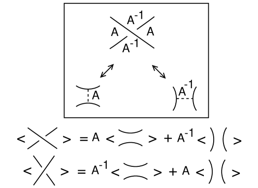 |
It is easy to see that Properties and define the calculation of the bracket on arbitrary link diagrams. The choices of coefficients ( and ) and the value of make the bracket invariant under the Reidemeister moves II and III. Thus Property is a consequence of the other two properties.
In computing the bracket, one finds the following behaviour under Reidemeister move I:
and
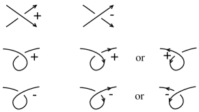
where denotes a curl of positive type as indicated in Figure 2, and indicates a curl of negative type, as also seen in this figure. The type of a curl is the sign of the crossing when we orient it locally. Our convention of signs is also given in Figure 2. Note that the type of a curl does not depend on the orientation we choose. The small arcs on the right hand side of these formulas indicate the removal of the curl from the corresponding diagram.
The bracket is invariant under regular isotopy and can be normalized to an invariant of ambient isotopy by the definition
where we chose an orientation for , and where is the sum of the crossing signs of the oriented link . is called the writhe of . The convention for crossing signs is shown in Figure 2.
 |
Remark. By a change of variables one obtains the original Jones polynomial, for oriented knots and links from the normalized bracket:
The bracket model for the Jones polynomial is quite useful both theoretically and in terms of practical computations. One of the neatest applications is to simply compute for the trefoil knot and determine that is not equal to That computation shows that the trefoil is not ambient isotopic to its mirror image, a fact that is much harder to prove by classical methods.
The State Summation. In order to obtain a closed formula for the bracket, we now describe it as a state summation. Let be any unoriented link diagram. Define a state, , of to be a choice of smoothing for each crossing of There are two choices for smoothing a given crossing, and thus there are states of a diagram with crossings. In a state we label each smoothing with or according to the left-right convention discussed in Property (see Figure 1). The label is called a vertex weight of the state. There are two evaluations related to a state. The first one is the product of the vertex weights, denoted
The second evaluation is the number of loops in the state , denoted
Define the state summation, , by the formula
It follows from this definition that satisfies the equations
The first equation expresses the fact that the entire set of states of a given diagram is the union, with respect to a given crossing, of those states with an -type smoothing and those with an -type smoothing at that crossing. The second and the third equation are clear from the formula defining the state summation. Hence this state summation produces the bracket polynomial as we have described it at the beginning of the section.
The Temperley Lieb Algebra The Temperely Lieb algebra is an algebra over the ring and with multiplicative generators where is an identity element and the other generators satisfy the relations
where in the last equation, and runs through all values from to for the first two equations whenever they are defined. The additive structure of the Temperely-Lieb algebra makes it a free module over the base ring.
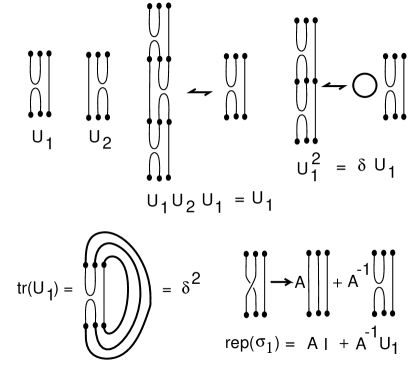
The Temperley-Lieb algebra can be interpreted as shown in Figure 3 in terms of planar connection patterns between two rows of points. In this Figure we illustrate the multiplicative relations and we show how a closure of a multiplicative element of the algebra leads to a collection of loops in the plane. There is a trace function defined in the diagrammatic interpretation by the formula
where is a product of gererators of the Temperley-Lieb algebra, and denotes the number of loops in the closure of the diagrammatic version of , as illustrated in Figure 3. This trace function is extended linearly to the whole algebra, and it has the property that for any elements and of the algebra.
Another way to think about the bracket polynomial is to first make a representation of the -strand Artin braid group to the Temperley-Lieb algebra on -strands and then take the trace ( as defined above) of this representation. The representation
is given by the formula
where denotes the -th braid generator and denotes the identity element in the Temperley-Lieb algebra. In Figure 3 we have illustrated this formula in the case This illustration should suffice for the reader to see what is our orientation convention for braid generators, and our convention for the standard closure of a diagrammatic element of the Temprely-Lieb algebra. This same notion of closure applies to braids. The reader will note that this braid representation parallels the definition of the bracket polynomial, so that the expansion formula for the bracket leads directly to the braid representation when applied to a diagram for the braid. The following Theorem is a consequence of this correspondence.
Theorem 1. Let be a braid in and let denote its standard closuure. Let denote the representation of the braid group discussed above, and let denote the trace on the Temperley-Lieb algebra discussed above. Then the bracket polynomial for the braid closure is given by the formula
 |
Remark. We can now explain how to produce unitary representations of the braid group in relation to the Temperley-Lieb algebra and the Jones polynomial. In order to make a unitary representation of the braid group, it is sufficient to find a representation of the Temperley-Lieb algebra to a complex vector space such that is a real and symmetric. Then, for any element on the unit circle in the complex plane, we see that is a unitary representaton of the Artin braid group. This statement follows from the fact, that under the above conditions is unitary. In the next section we give an elementary construction for a large class of unitary representations of the three-strand braid group, and then extend this class to include the Fibonacci model discussed in the Introduction.
3 Unitary Representations of the Braid Group and The Fibonacci Model
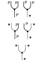
The constructions in this section are based on the combinatorics of the Fibonacci model. In this model we have a (mathematical) particle that interacts with itself either to produce or to produce a neutral particle . If is any particle then iteracts with to produce Thus acts as an identity trasformation. These rules of interaction are illustrated in Figure 4.
 |
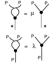 |
The braiding of two particles is measured in relation to their interaction. In Figure 5 we illustrate braiding of with itself in relation to the two possible interactions of with itself. If interacts to produce , then the braiding gives a phase factor of If interacts to produce , then the braiding gives a phase factor of We assume at the outset that and are unit complex numbers. One should visualize these particles as moving in a plane and the diagrams of interaction are either creations of two particles from one particle, or fusions of two particles to a single particle (depending on the choice of temporal direction). Thus we have a braiding matrix for these “local” particle interactions:
written with respect to the basis for this space of particle interactions.
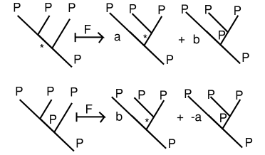
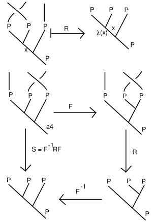
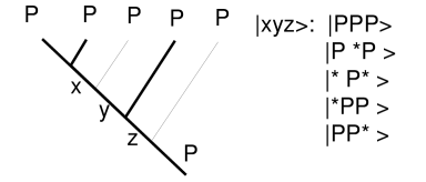
We want to make this braiding matrix part of a larger representation of the braid group. In particular, we want a representation of the three-strand braid group on the process space illustrated in Figure 6. This space starts with three particles and considers processes associated in the patttern with the stipulation that the end product is . The possible pathways are illustrated in Figure 6. They correspond to and This process space has dimension two and can support a second braiding generator for the second two strands on the top of the tree. In order to articulate the second braiding we change basis to the process space corresponding to as shown in Figures 7 and 8. The change of basis is shown in Figure 7 and has matrix as shown below. We want a unitary representation of three-strand braids so that and See Figure 8. We take the form of the matrix as follows.
where with and real. This form of the matrix for the basis change is determined by the requirement that is symmetric with . The symmetry of the change of basis formula essentially demands that If is real, symmetric and , then is unitary. Since is unitary we see that is also unitary. Thus, if is constructed in this way then we obtain a unitary representation of
Now we try to simultaneously construct an and construct a representation of the Temperley-Lieb algebra as described in section 2. We begin by noting that
where Thus where so that For the Temperley-Lieb representation, we want as explained in section 2. Hence we need which implies that With this restriction on we have the Temperley-Lieb representation and the corresponding unitary braid group representation for -strand braids and the -strand Temperley-Lieb algebra.
 |
 |
 |
Now we can go on to and via with We must examine , and We find that
as desired and
Thus and since and with and ( denotes transpose), we see that
Similarly Thus, we need and so we shall take With this choice, we have a representation of the Temperley-Lieb algebra so that and gives a unitary representation of the braid group when and is real. This last reality condition is equivalent to the inequality
which is satisfied for infinitely many values of in the ranges
With these choices we have
real and unitary, and for the Temperley-Lieb algebra,
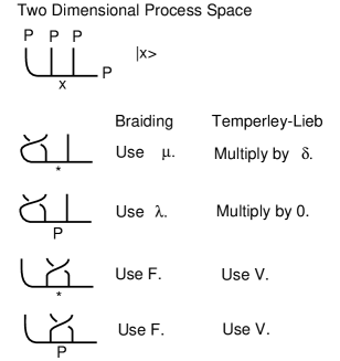
Now examine Figure 9. Here we illustrate the action of the braiding and the Temperley-Lieb Algebra on the first Fibonacci process space with basis Here we have and as described above. Thus we have a representation of the braid group on three strands and a representation of the Temperley-Lieb algebra on three strands with no further restrictions on
 |
 |
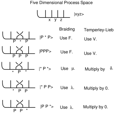 |
So far, we have arrived at exactly the -strand braid representations that we used in our papers [12, 13] giving a quantum algorithm for the Jones polynomial for three-strand braids. In this paper we are working in the context of the Fibonacci process spaces and so we wish to see how to make a representation of the Temperley-Lieb algebra to this model as a whole, not restricting ourselves to only three strands. The generic case to consider is the action of the Temperley-Lieb algebra on process spaces of higher dimension as shown in Figures 10 and 11. In the Figure 11 we have illustrated the triplets from the previous figure as part of a possibly larger tree and have drawn the strings horizontally rather than diagonally. In this figure we have listed the effects of braiding the vertical strands and . We see from this figure that the action of the Temperley-Lieb algebra must be as follows:
Here we have denoted this action as because it connotes the action on the third and fourth vertical strands in the sequences shown in Figure 11. Note that in a larger sequence we can recognize by examining the triplet surrounding the -th element in the sequence, just as the pattern above is governed by the elements surrounding the second element in the sequence. For simplicity, we have only indicated three elements in the sequences above. Note that in a sequence for the Fibonacci process there are never two consecutive appearances of the neutral element
We shall refer to a sequence of and as a Fibonacci sequence if it contains no consecutive appearances of . Thus is a Fibonacci sequence. In working with this representation of the braid group and Temperley-Lieb algebra, it is convenient to assume that the ends of the sequence are flanked by as in Figures 10 and 11 for sequences of length It is convenient to leave out the flanking ’s when notating the sequence.
Using these formulas we can determine conditions on such that this is a representation of the Temperley-Lieb algebra for all Fibonacci sequences. Consider the following calculation:
Thus we see that in order for we need that
It is easy to see that is the only remaining condition needed to make sure that the action of the Temperley-Lieb algebra extends to all Fibonacci Model sequences.
Note that Thus we require that
When we have the solutions However, for the reality of we require that ruling out the choice When we have the solutions This leaves only where (the Golden Ratio) as possible values for that satisfy the reality condition for Thus, up to a sign we have arrived at the well-known value of (the Fibonacci model) as essentially the only way to have an extension of this form of the representation of the Temperley-Lieb algebra for strands. Let’s state this positively as a Theorem.
Theorem 2. Let be the complex vector space with basis where each equals either or and there do not occur two consecutive appearances of in the sequence We refer to this basis for as the set of Fibonacci sequences of length Then the dimension of is equal to where is the -th Fibonacci number: and Let where Let and Then the Temperley-Lieb algebra on strands with loop value acts on via the formulas given below. First we give the left-end actions.
Then we give the general action for the middle strands.
Finally, we give the right-end action.
Remark. Note that the left and right end Temperley-Lieb actions depend on the same basic pattern as the middle action. The Fibonacci sequences should be regarded as flanked left and right by ’s just as in the special cases discussed prior to the proof of Theorem .
Corollary. With the hypotheses of Theorem , we have a unitary representation of the Artin Braid group to , given by the formulas
where where the connote the representation of the Temperley-Lieb algebra on the space of Fibonacci sequences as described in the Theorem above.
Remark. The Theorem and Corollary give the original parameters of the Fibonacci model and shows that this model admits a unitary representation of the braid group via a Jones representation of the Temperley-Lieb algebra.
In the original Fibonacci model [11], there is a basic non-trivial recoupling matrix
where is the golden ratio and . The local braiding matrix is given by the formula below with
This is exactly what we get from our method by using and Just as we have explained earlier in this paper, the simplest example of a braid group representation arising from this theory is the representation of the three strand braid group generated by and (Remember that ). The matrices and are both unitary, and they generate a dense subset of supplying the local unitary transformations needed for quantum computing. The full braid group representation on the Fibonacci sequences is computationally universal for quantum computation. In our earlier paper [11] we gave a construction for the Fibonacci model based on Temperely-Lieb recoupling theory. In this paper, we have reconstructed the Fibonacci model on the more elementary grounds of the representation of the Temperley-Lieb algebra summarized in the statement of the Theorem and its Corollary.
References
- [1] D. Aharonov, V. Jones, Z. Landau, A polynomial quantum algorithm for approximating the Jones polynomial, quant-ph/0511096.
- [2] M. Freedman, A magnetic model with a possible Chern-Simons phase, quant-ph/0110060v1 9 Oct 2001, (2001), preprint
- [3] M. Freedman, Topological Views on Computational Complexity, Documenta Mathematica - Extra Volume ICM, 1998, pp. 453–464.
- [4] M. Freedman, M. Larsen, and Z. Wang, A modular functor which is universal for quantum computation, quant-ph/0001108v2, 1 Feb 2000.
- [5] M. H. Freedman, A. Kitaev, Z. Wang, Simulation of topological field theories by quantum computers, Commun. Math. Phys., 227, 587-603 (2002), quant-ph/0001071.
- [6] M. Freedman, Quantum computation and the localization of modular functors, quant-ph/0003128.
- [7] V.F.R. Jones, A polynomial invariant for links via von Neumann algebras, Bull. Amer. Math. Soc. 129 (1985), 103–112.
- [8] L.H. Kauffman, State models and the Jones polynomial, Topology 26 (1987), 395–407.
- [9] L. H. Kauffman and S. J. Lomonaco Jr., Spin Networks and anyonic topological computing, In “Quantum Information and Quantum Computation IV”, (Proceedings of Spie, April 17-19,2006) edited by E.J. Donkor, A.R. Pirich and H.E. Brandt, Volume 6244, Intl Soc. Opt. Eng., pp. 62440Y-1 to 62440Y-12.
- [10] L. H. Kauffman and S. J. Lomonaco Jr., Spin Networks and anyonic topological computing II, In “Quantum Information and Quantum Computation V”, (Proceedings of Spie, April 10-12,2007) edited by E.J. Donkor, A.R. Pirich and H.E. Brandt, Volume 6573, Intl Soc. Opt. Eng., pp. 65730U-1 to 65730u-13.
- [11] L. H. Kauffman and S. J. Lomonaco Jr., - Deformed Spin Networks, Knot Polynomials and Anyonic Topological Quantum Computation, JKTR Vol. 16, No. 3 (March 2007), pp. 267-332.
- [12] L. H. Kauffman, Quantum computing and the Jones polynomial, math.QA/0105255, in Quantum Computation and Information, S. Lomonaco, Jr. (ed.), AMS CONM/305, 2002, pp. 101–137.
- [13] L.H. Kauffman and Samuel J. Lomonaco Jr. A Three-stranded quantum algorithm for the Jones polynonmial, in “Quantum Information and Quantum Computation V”, (Proceedings of Spie, April 2007) edited by E.J. Donkor, A.R. Pirich and H.E. Brandt, Intl Soc. Opt. Eng. , 65730T-1-16.
- [14] A. Kitaev, Anyons in an exactly solved model and beyond, arXiv.cond-mat/0506438 v1 17 June 2005.
- [15] G. Moore and N. Read, Non-abelions in the fractional quantum Hall effect, Nuclear PhysicsB 360 (1991), 362-396.
- [16] A. Marzuoli and M. Rasetti, Spin network quantum simulator, Physics Letters A 306 (2002) 79–87.
- [17] J. Preskill, Topological computing for beginners, (slide presentation), Lecture Notes for Chapter 9 - Physics 219 - Quantum Computation. http://www.iqi.caltech.edu/ preskill/ph219
- [18] P. W. Shor and S. P. Jordan, Estimating Jones polynomials is a complete problem for one clean qubit. arxiv:0707.2831v1 [quqnt-ph] 19 Jul 2007.
- [19] F. Wilczek, Fractional Statistics and Anyon Superconductivity, World Scientific Publishing Company (1990).
- [20] E. Witten, Quantum field Theory and the Jones Polynomial, Commun. Math. Phys.,vol. 121, 1989, pp. 351-399.