$q$-Gaussians in the porous-medium equation: stability and time evolution

Abstract

The stability of $q$-Gaussian distributions as particular solutions of the linear diffusion equation and its generalized nonlinear form, $\frac{\partial P(x,t)}{\partial t}=D\frac{\partial^{2}[P(x,t)]^{2-q}}{\partial x^{2}}$, the porous-medium equation, is investigated through both numerical and analytical approaches. It is shown that an initial $q$-Gaussian, characterized by an index $q_{i}$, approaches the final, asymptotic solution, characterized by an index $q$, in such a way that the relaxation rule for the kurtosis evolves in time according to a $q$-exponential, with a relaxation index $q_{\rm rel}\equiv q_{\rm rel}(q)$. In some cases, particularly when one attempts to transform an infinite-variance distribution ($q_{i}\geq 5/3$) into a finite-variance one ($q<5/3$), the relaxation towards the asymptotic solution may occur very slowly in time. This fact might shed some light on the slow relaxation, for some long-range-interacting many-body Hamiltonian systems, from long-standing quasi-stationary states to the ultimate thermal equilibrium state.

Keywords: Anomalous Diffusion, Porous Medium Equation, Nonextensive Thermostatistics.

I Introduction

The linear diffusion equation, which is one of the most important differential equations of classical physics, rules the time evolution of the probability distribution associated with a particle diffusing in a homogeneous medium. This probability distribution spreads in time, with its second moment increasing linearly with time, being appropriate for a description of many physical phenomena, usually classified as normal diffusion. Such an equation presents a structure very common in physics, e.g., it is analogous to the heat-conduction equation, and by introducing an additional term, characterizing an external harmonic force field, it becomes the linear Fokker-Planck equation (FPE) VanKampen:81 ; Risken:89 . The linear FPE is essentially associated with the Boltzmann-Gibbs (BG) formalism, in the sense that the Boltzmann distribution, which is usually obtained through the maximization of the BG entropy under certain constraints, also appears as the stationary solution of the linear FPE Risken:89 ; Cover:91 . However, such simple linear equations are not appropriate for dealing with many physical situations, characterized by anomalous diffusion, like particle transport in disordered media Muskat:37 and motion in optical lattices Lutz:03 .

Due to the recent advance in computer technology, some problems in physics that remained unexplored for a long time are now under investigation, at least from the computational point of view. In particular, one should single out those problems described in terms of nonlinear differential equations, which have led to new features and interesting puzzles that keep challenging many physicists nowadays. The nonlinear FPEs Frank:05 , which are formulated by introducing modifications in the standard FPE, appear naturally as good candidates for describing anomalous-transport processes. In most cases, the nonlinear FPEs are proposed as simple phenomenological generalizations of the linear FPE Plastino:95 ; Tsallis:96 ; Borland:98b ; Frank:99 , although it is possible to obtain them through approximations in the master equation Curado:03 ; Nobre:04 ; Schwaemmle:07c . Recently, a relation involving quantities of the FPE and entropic forms was proposed, in a proof of the H-theorem using nonlinear FPEs Schwaemmle:07c ; Schwaemmle:07b ; as a consequence of such a relation, one obtains that the BG entropy is directly connected to the linear FPE, whereas generalizations of the BG entropy are associated with nonlinear FPEs Schwaemmle:07c ; Schwaemmle:07b . This reinforces the belief that nonlinear FPEs are intimately related to nonextensive statistical mechanics next:04 ; next:05 .

If one considers the nonlinear FPE associated with the nonadditive entropy $S_{q}$ Tsallis:88 in the absence of an external force field, one gets Plastino:95 ; Tsallis:96 the porous-medium equation (also known as nonlinear heat equation) Vazquez:06 ,

$$\frac{\partial P(x,t)}{\partial t}=D\frac{\partial^{2}[P(x,t)]^{2-q}}{\partial x^{2}}~{},$$ (1)

which governs the time evolution of the probability distribution $P(x,t)$ for finding a diffusing particle in the position $x$ at time $t$, in a medium characterized by a diffusion constant $D$; the linear diffusion equation comes out as a particular case, by considering $q=1$. It should be noticed that, within a numerical analysis, as will be one of the main purposes of the present work, the parameter $q$ above corresponds to the index associated with the asymptotic behavior of the solution of Eq. (1), known as a $q$-Gaussian, related to the nonadditive entropy Tsallis:88 .

Recently, classical inertial long-range-interaction Hamiltonian systems have attracted a lot of attention LatoraRuffo:98 ; Anteneodo:98 ; Moyano:06 ; Pluchino:07 ; Pluchino:08 ; nobretsallis:03 ; nobretsallis:04 ; Ruffo:07 ; Ruffo:07b . These systems consist in assemblies of classical rotators, which evolve in time, e.g., in a plane (XY rotators LatoraRuffo:98 ; Anteneodo:98 ; Moyano:06 ; Pluchino:07 ; Pluchino:08 ), or in a sphere (Heisenberg rotators nobretsallis:03 ; nobretsallis:04 ). For the case of infinite-range ferromagnetic interactions, i.e., in the mean-field limit, one may calculate thermodynamic properties analytically, within the BG canonical ensemble, and in particular, verify the existence of a continuous phase transition. The interesting aspect about these systems is that one may compute their time evolution through a direct integration of their equations of motion, without introducing a priori any phenomenological dynamic rules, but just using Newton’s law. A quite curious behavior has shown up by starting the numerical-integration procedure with initial conditions very different from those required in the standard BG equilibrium: the system gets trapped in metastable states, before approaching their corresponding terminal thermal equilibria. These metastable states are characterized by “kinetic temperatures” that are different from the equilibrium ones; besides that, the duration of such states increases with the number of rotators, $N$. Hence, if one considers the thermodynamic limit ($N\rightarrow\infty$) before the long-time limit, these systems will remain in these metastable states and will never reach their terminal equilibrium state, in such a way that the phase space will not be equally and completely covered, i.e., these systems are nonergodic. Moreover, in such metastable states, the maximum Lyapunov exponent approaches zero, as $N\rightarrow\infty$ Anteneodo:98 ; nobretsallis:03 , contrary to what is expected in a standard BG equilibrium state. For finite values of $N$, at large enough – but realizable computational times – one approaches a state that is presumably the terminal thermal equilibrium state, in the sense that its kinetic temperature is in agreement with the one obtained through the BG canonical-ensemble calculations. However, although the kinetic temperature of the long-time limit state agrees with the one obtained from the canonical-ensemble calculations, other properties may still not coincide with those expected in a true equilibrium BG state; as an example, one has a recent analysis of the angles described by the infinite-range-interaction XY rotator model, for which their distribution in the long-time-limit is well-fitted by a $q$-Gaussian, with $q\approx 1.5$ Moyano:06 . This suggests that the BG equilibrium state is approached through different steps, one of them being the attainment of the equilibrium temperature; a relevant question concerns how long will it take for the system to reach completely the final BG equilibrium state.

In the present work we search for clues on how the approach to equilibrium occurs in the above-mentioned Hamiltonian models, by investigating the time evolution of probability distributions in a much simpler system, i.e., the porous-medium equation. For that, we integrate Eq. (1), starting the integration procedure with an initial distribution different from its asymptotic solution. In particular, we will consider as initial distribution a $q$-Gaussian characterized by an entropic index $q_{i}$ ($q_{i}\neq q$), and will follow the time evolution of such a distribution towards the final (i.e., asymptotic) $q$-Gaussian, specified by the index $q_{f}$, that hopefully, $q_{f}\equiv q$. Exploring the stability of $q$-Gaussians in an environment given by Eq. (1) may help to understand why metastable states that appear in the infinite-range-interaction models of rotators remain stable over such long periods. In the following section we discuss the exact solutions of the porous-medium equation and their connection to anomalous diffusion. In Sec. III we introduce generalized moments, as well as a generalized kurtosis, which are more appropriate for dealing with fat-tailed distributions. In Sec. IV we analyze the time evolution of a probability distribution by following the linear diffusion equation [$q=1$ in Eq. (1)], provided that the initial distribution is given by a $q$-Gaussian with $q_{i}\neq 1$. In Sec. V we carry a similar analysis for the porous-medium equation [$q\neq 1$ in Eq. (1)], having as initial state a $q$-Gaussian with $q_{i}\neq q$. In Secs. IV and V we show, by monitoring the time evolution of the kurtosis, that the approach to the final $q$-Gaussian obeys a $q$-exponential function, characterized by a relaxation index $q_{\rm rel}$. At this point, it is important to stress that in the present work we deal, in principle, with four indexes: (i) the index $q$ defined by Eq. (1); (ii) $q_{i}$, associated with the initial $q$-Gaussian distribution; (iii) $q_{f}$, associated with the final $q$-Gaussian distribution (for which one expects, $q_{f}\equiv q$); (iv) $q_{\rm rel}$, related to the $q$-exponential of the relaxation towards the asymptotic distribution. However, in the present work we have found no evidence, either in our analytical or numerical approaches, of $q_{f}\neq q$; hence, we shall assume from now on that $q_{f}\equiv q$. Therefore, we will restrict our analysis to three indexes, namely, $q,\,q_{i}$, and $q_{\rm rel}$, as defined above. Finally, in the last section we present our main conclusions.

II Exact solutions of the porous-medium equation

In this section we discuss briefly the well-known exact solutions for a diffusing particle following Eq. (1). In order to guarantee the preservation of the normalization for all times $t$, one should impose the probability distribution, together with its first derivative to be zero at infinity,

$$P(x,t)|_{x\rightarrow\pm\infty}=0~{};\quad\left.{\partial P(x,t)\over\partial x}\right|_{x\rightarrow\pm\infty}=0~{},\quad(\forall t)~{}.$$ (2)

If one chooses a perfectly localized particle as the initial state, $P(x,0)=\delta(x_{0})$ [$\delta(x)$ denotes the delta-function], then, following Refs. Plastino:95 ; Tsallis:96 , one can write the solution of Eq. (1), satisfying the conditions of Eq. (2), in terms of a $q$-Gaussian,

$$P(x,t)=Z_{q}b_{q}(t)\ \text{e}^{-b_{q}^{2}(t)(x-x_{0})^{2}}_{q}~{},\quad\text{for }q<3~{},\\$$ (3)

where $\text{e}^{x}_{q}=\left[1+(1-q)x\right]_{+}^{1/(1-q)}$ (herein, the bracket $[C]_{+}=C$, for $C\geq 0$, and is zero otherwise) represents the $q$-generalization of the standard exponential function that is recovered in the limit $q\rightarrow 1$; its inverse, known as the $q$-logarithmic function, is given by $\ln_{q}x=(x^{1-q}-1)/(1-q)$. This solution presents a compact support for $q<1$, and exhibits power-law tails for $q>1$. The time-dependent part of the solution, $b_{q}(t)$, and the normalization constant, $Z_{q}$, are given, respectively, by

$$b_{q}(t)=\left[2D(2-q)(3-q)Z_{q}^{1-q}\ t\right]^{1/(q-3)}~{},\quad(D(2-q)>0)~{},$$ (4)

$$Z_{q}=\begin{cases}\sqrt{\frac{|D|(q-1)}{\pi}}~{}\frac{\Gamma\left(\frac{1}{q-1}\right)}{\Gamma\left(\frac{1}{q-1}-\frac{1}{2}\right)}~{},\quad&\text{for }1<q<3~{},\\ \sqrt{\frac{D}{\pi}}~{},\quad&\text{for }q=1~{},\\ \sqrt{\frac{D(1-q)}{\pi}}~{}\frac{\Gamma\left(1+\frac{1}{1-q}\right)}{\Gamma\left(\frac{3}{2}+\frac{1}{1-q}\right)}~{},\quad&\text{for }q<1~{},\end{cases}$$ (5)

where $\Gamma(x)$ represents the Gamma-function.

The diffusion is usually characterized by the time behavior of the second moment of the distribution, which is given by $<x^{2}>=(b_{q}(t))^{-2}$, scaling as $t^{2/(3-q)}$. Hence, $q=1$ yields a linear increase in time, i.e., normal diffusion, whereas Eq. (1) leads to anomalous diffusion for $q\neq 1$. Within anomalous diffusion, one may distinguish super-diffusion ($q>1$), characterized by long-tailed distributions, from sub-diffusion ($q<1$), related to compact-support distributions.

If one starts the numerical integration of Eq. (1) with $P(x,0)=\delta(x_{0})$, one follows the corresponding $q$-Gaussian, associated with $<x^{2}>\sim t^{2/(3-q)}$. However, if one uses as an initial distribution a $q$-Gaussian specified by an index $q_{i}\neq q$, the numerical procedure will take some time to gradually change from such an initial, to the final $q$-Gaussian distribution. Herein, we will be particularly interested in measuring the time that the system takes to approach its final distribution asymptotically. Therefore, different initial states of the system are expected to yield different relaxation behavior. In the analysis that follows, the solution presented in Eqs. (3)–(5) will be our reference and its kurtosis, to be introduced in the next section, will be an important quantity to characterize the relaxation behavior.

III Generalized moments and kurtosis

The kurtosis is usually defined in terms of the ratio between the fourth, and the square of the second moments of a given distribution. However, for the $q$-Gaussian distribution defined in the previous section, one gets divergences in its even moments, in such a way that the second moment diverges for $q\geq 5/3$, whereas the fourth moment diverges for $q\geq 7/5$. Therefore, the standard definitions of moments and kurtosis become useless for certain ranges of $q$ values. In the present section, we introduce generalized moments, and apply them in a definition of a generalized kurtosis.

Let us define the generalized $n$-th moment of a given distribution as,

$$<x^{n}>_{r}~{}=~{}{\int\limits_{-\infty}^{\infty}dx~{}x^{n}[P(x,t)]^{r}\over\int\limits_{-\infty}^{\infty}dx[P(x,t)]^{r}}~{},$$ (6)

where $n$ is a positive integer and $r\geq 0$. For the $q$-Gaussian distribution, defined in the previous section, one has

$$<x^{2}>_{r}= \begin{cases}\frac{1}{2}\frac{b_{q}^{-2}(t)}{q-1}\frac{\Gamma\left(\frac{r}{q-1}-\frac{3}{2}\right)}{\Gamma\left(\frac{r}{q-1}-\frac{1}{2}\right)}~{},&\text{for }0<(q-1)<\frac{2}{3}r~{},\\ \frac{1}{2}\frac{b_{1}^{-2}}{r}~{},&\text{for }q=1~{},\\ \frac{1}{2}\frac{b_{q}^{-2}(t)}{1-q}\frac{\Gamma\left(\frac{r}{1-q}+\frac{3}{2}\right)}{\Gamma\left(\frac{r}{1-q}+\frac{5}{2}\right)}~{},&\text{for }q<1~{},\end{cases}$$ (7)

$$<x^{4}>_{r}= \begin{cases}\frac{3}{4}\frac{b_{q}^{-4}(t)}{(q-1)^{2}}\frac{\Gamma\left(\frac{r}{q-1}-\frac{5}{2}\right)}{\Gamma\left(\frac{r}{q-1}-\frac{1}{2}\right)}~{},&\text{for }0<(q-1)<\frac{2}{5}r~{},\\ \frac{3}{4}\frac{b_{1}^{-4}}{r^{2}}~{},&\text{for }q=1~{},\\ \frac{3}{4}\frac{b_{q}^{-4}(t)}{(1-q)^{2}}\frac{\Gamma\left(\frac{r}{1-q}+\frac{3}{2}\right)}{\Gamma\left(\frac{r}{1-q}+\frac{7}{2}\right)}~{},&\text{for }q<1~{}.\end{cases}$$ (8)

Considering the above moments, one may define the following generalized kurtosis,

$$\kappa_{r,s}(q)=\frac{<x^{4}>_{r}}{(<x^{2}>_{s})^{2}}=\begin{cases}3\frac{\Gamma\left(\frac{r}{q-1}-\frac{5}{2}\right)\left(\Gamma\left(\frac{s}{q-1}-\frac{1}{2}\right)\right)^{2}}{\Gamma\left(\frac{r}{q-1}-\frac{1}{2}\right)\left(\Gamma\left(\frac{s}{q-1}-\frac{3}{2}\right)\right)^{2}}~{},&\text{for }0<(q-1)<\text{min}\left(\frac{2}{3}r,\ \frac{2}{5}s\right)~{},\\ 3\frac{s^{2}}{r^{2}}~{},&\text{for }q=1~{},\\ 3\frac{\Gamma\left(\frac{r}{1-q}+\frac{3}{2}\right)\left(\Gamma\left(\frac{s}{1-q}+\frac{5}{2}\right)\right)^{2}}{\Gamma\left(\frac{r}{1-q}+\frac{7}{2}\right)\left(\Gamma\left(\frac{s}{1-q}+\frac{3}{2}\right)\right)^{2}}~{},&\text{for }q<1~{},\end{cases}$$ (9)

If one uses the property $\Gamma(x+1)=x\Gamma(x)$, it is possible to write this kurtosis in a form that covers all three possibilities above,

$$\kappa_{r,s}(q)=3\ \frac{(2s-3(q-1))^{2}}{(2r-3(q-1))(2r-5(q-1))}~{},\quad\left[(q-1)<\text{min}\left(\frac{2}{3}r,\ \frac{2}{5}s\right)\right]~{}.$$ (10)

In the numerical integration of Eq. (1) the initial $q$-Gaussian, characterized by an entropic index $q_{i}$ ($q_{i}\neq q$), will evolve in time towards the final $q$-Gaussian. Obviously, it is desirable to have $\kappa_{r,s}(q)$ always finite when the parameter $q$ varies in the interval $q_{i}\rightarrow q$; unfortunately, this is not possible in some cases, and for this purpose, one has to choose the exponents $r$ and $s$ conveniently. Herein, we choose these exponents by giving preference to a finite kurtosis in the asymptotic limit ($t\gg 1$).

Figure 1: The kurtosis at the beginning of the numerical procedure [Eq. (11)], characterized by linear diffusion in the asymptotic regime ($q=1$), $\kappa_{1,1}(q_{i})$, is exhibited versus $q_{i}$ (dashed line). Also shown is the kurtosis at the final regime, $\kappa_{\bar{r},q}(q)$ versus $q$ (full line). Notice that the standard Gaussian value, $\kappa_{1,1}(1)=3$, is recovered from both cases.

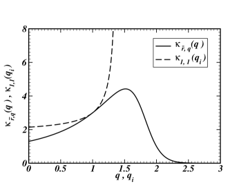
In a recent proof of a generalized central-limit theorem, $q$-Gaussian distributions appear as a result of given composition rules Umarov:06 ; Vignat:07 . Inspired by some results of this theorem, we will consider the choices $s=q$ and $r=\bar{r}\equiv(q+1)/(3-q)$; the choice $r=\bar{r}$ ensures a finite second moment in the asymptotic limit ($t\gg 1$). Substituting these quantities in Eq. (10), one gets the following expression for the kurtosis at the beginning of the numerical procedure,

$$\kappa_{\bar{r},q}(q_{i})=3\ \frac{[3-q]^{2}[2q-3(q_{i}-1)]^{2}}{[11-q-3q_{i}(3-q)][17-3q-5q_{i}(3-q)]}~{},$$ (11)

which is finite, provided that $(q_{i}-1)<\text{min}\left[(2/5)(q+1)/(3-q),(2/3)q\right]$. An interesting particular case of Eq. (11) is the one characterized by linear diffusion in the asymptotic regime, i.e., $q=1$, yielding $\kappa_{1,1}(q_{i})=3\cdot(5-3q_{i})/(7-5q_{i})$, which leads to a divergence at $q_{i}=7/5$, as shown in Fig. 1.

The same choices for the exponents $r$ and $s$ yield the kurtosis of Eq. (10) in the asymptotic regime,

$$\kappa_{\bar{r},q}(q)=3\ \frac{(3-q)^{4}}{(3q^{2}-10q+11)(5q^{2}-18q+17)}~{}.$$ (12)

In Fig. 1 we exhibit the kurtosis above versus $q$, showing that, as expected, it does not diverge.

Therefore, when the $q$-Gaussian changes between the two entropic indices $q_{i}\rightarrow q$, the kurtosis evolves in time, changing its behavior between those described in Eqs. (11) and (12), respectively; although the kurtosis may be infinite during its time evolution, it will be finite in the asymptotic limit.

IV $q=1$ and arbitrary initial distributions

In this section we restrict our study to the linear diffusion equation [Eq. (1) with $q=1$], analyzing the time evolution of different initial states given by $q$-Gaussians [cf. Eq. (3)], characterized by distinct entropic indexes $q_{i}$.

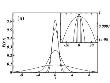
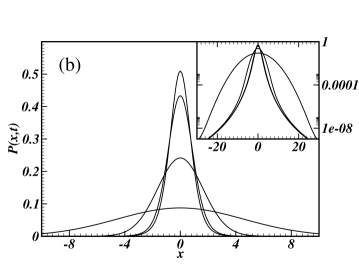
As an illustration, we exhibit in Fig 2 the time evolution of $P(x,t)$, starting the numerical integration with two typical $q$-Gaussians, namely, $q_{i}=3/4$ [Fig 2(a)] and $q_{i}=5/4$ [Fig 2(b)]. On the linear scale, one observes no notable difference between the time evolution of these probability distributions. Nevertheless, on the log-linear scale (cf. insets of Fig. 2), one sees clearly that the initial distribution relaxes faster to the Gaussian limit in the case $q_{i}=3/4$, whereas the fat tails remain stable over a longer period for $q_{i}=5/4$. In particular, in this later case, one notices the presence of an inflection point, characteristic of $q$-Gaussians with $q>1$, at intermediate times (i.e., in the transient regime), which disappears when the distribution approaches the Gaussian limit.

Figure 2: Time evolution of the probability distribution associated with the linear diffusion equation at typical times, $t=0,0.1,1,10$ (from top to bottom). The system is initialized with $q$-Gaussians, characterized by initial entropic indexes $q_{i}=0.75$ (a) and $q_{i}=1.25$ (b). In the insets we exhibit the same distributions on a semi-logarithmic scale.

In what concerns the kurtosis, $\kappa_{1,1}(q_{i})$, introduced in the previous section, it may be calculated analytically, for $q_{i}<7/5$. This quantity enables a measure of the time the system needs to reach asymptotically the Gaussian distribution; from now on, we will indicate its time dependence explicitly, by referring to it as $\kappa_{1,1}(q_{i},t)$. As we deal here with a linear partial differential equation, the calculation of the moments may be carried out exactly by the use of the Green’s function method. The final distribution is a standard Gaussian,

$$P(x,t)=\frac{1}{2\sqrt{D\pi t}}\exp\left[-\frac{(x-x_{0})^{2}}{4Dt}\right]~{},$$ (13)

and the corresponding Green’s function is given by Mathews:70 ,

$$G(y,x|t)=\frac{1}{2\sqrt{\pi t}}\exp\left[{-\frac{(x-y)^{2}}{4Dt}}\right]~{},$$ (14)

from which one obtains the time-dependent solution of the diffusion equation,

$$P(x,t)=\int\limits_{-\infty}^{\infty}G(y,x|t)P(y,0)dy~{},$$ (15)

for arbitrary initial distributions $P(x,0)$. Let us now calculate the $n$-th moment of the time-dependent solution,

$$<x^{n}>_{1} = \int\limits_{-\infty}^{\infty}dx~{}x^{n}\int\limits_{-\infty}^{\infty}dy~{}G(y,x|t)P(y,0)=\int\limits_{-\infty}^{\infty}dyP(y,0)\int\limits_{-\infty}^{\infty}dx~{}x^{n}G(y,x|t)$$

$$=\frac{1}{2\sqrt{\pi t}}\int\limits_{-\infty}^{\infty}dy~{}P(y,0)\int\limits_{-\infty}^{\infty}dx~{}(x-y)^{n}\exp\left({-\frac{x^{2}}{4Dt}}\right)~{}.$$ (16)

Using Eq. (16), we obtain the time evolution of the moments of $P(x,t)$ for arbitrary initial functions $P(x,0)$, just by calculating standard Gaussian integrals. In order to obtain the kurtosis, we calculate the second and fourth moments, respectively,

$$<x^{2}>_{1}=\int\limits_{-\infty}^{\infty}dyP(y,0)\left(y^{2}+2t\right)=\bar{y^{2}}+2t~{},$$ (17)

and

$$<x^{4}>_{1}=\int\limits_{-\infty}^{\infty}dyP(y,0)\left(y^{4}+12ty^{2}+12t^{2}\right)=\bar{y^{4}}+12\bar{y^{2}}t+12t^{2}~{},$$ (18)

where $\bar{y^{2}}$ and $\bar{y^{4}}$ denote the standard second and fourth moments of the initial distribution $P(x,0)$. Using these results, the kurtosis becomes,

$$\kappa_{1,1}(q_{i},t)=\frac{<x^{4}>_{1}}{(<x^{2}>_{1})^{2}}=\frac{\bar{y^{4}}+12t(\bar{y^{2}}+t)}{(\bar{y^{2}}+2t)^{2}}~{}.$$ (19)

Therefore, the kurtosis’ asymptotic value, $\lim_{t\rightarrow\infty}\kappa_{1,1}(1,t)=3$, is approached according to,

$$\kappa_{1,1}(q_{i},t)-3=\frac{\bar{y^{4}}-3(\bar{y^{2}})^{2}}{(\bar{y^{2}}+2t)^{2}}~{}.$$ (20)

The equation above yields the kurtosis in terms of the second and fourth moments of initial $q$-Gaussians, provided that $q_{i}<7/5$. Notice that $\kappa_{1,1}(q_{i})-3$ is negative, for $q_{i}<1$, and positive, for $1<q_{i}<7/5$. Defining $b\equiv b_{q_{i}}(t=0)=$ constant, and using Eqs. (7) and (8),

$$\bar{y^{2}}=\frac{b^{-2}}{5-3q_{i}}~{},\quad(q_{i}<5/3),$$ (21)

$$\bar{y^{4}}=3\frac{b^{-4}}{(5-3q_{i})(7-5q_{i})}~{},\quad(q_{i}<7/5),$$ (22)

and thus,

$$\kappa_{1,1}(q_{i},t)-3=6\ \frac{q_{i}-1}{7-5q_{i}}\ \frac{1}{[1+2b^{2}(5-3q_{i})t]^{2}}=6\ \frac{q_{i}-1}{7-5q_{i}}\ \text{e}^{-4b^{2}(5-3q_{i})t}_{3/2}~{},\quad(q_{i}<7/5).$$ (23)

The equation above indicates that all initial $q$-Gaussians, characterized by $q_{i}<7/5$, present a kurtosis that will relax to the standard Gaussian ($q=1$), following $q$-exponentials with the same relaxation index, $q_{\rm rel}=3/2$, but different relaxation times, $1/[4b^{2}(5-3q_{i})]$. Such a dependence of the arguments of these $q$-exponential functions on the initial entropic index $q_{i}$ imply on longer relaxation times for larger values of $q_{i}$. This is in agreement with the results of the numerical calculation exibited in Fig 2, corresponding to the time evolution of two distributions initialized as $q$-Gaussians, with $q_{i}=3/4$ and $q_{i}=5/4$, respectively.

Figure 3: Time evolution of the kurtosis obtained by a numerical integration of the linear diffusion equation [Eq. (1) with $q=1$] is compared to the one of the kurtosis $\kappa_{1,1}(q_{i},t)$, calculated exactly [Eq. (23)], for typical values of $q_{i}$. The data is exhibited in (a) linear-linear, (b) log-log and $q$-logarithm-linear [inset of figure (b)] plots. The straight lines in the inset of figure (b) [notice that the data for $q_{i}=0.6$ and $q_{i}=0.8$ appear essentially superposed] ensure the index $q_{\rm rel}=3/2$ of the relaxation process, and their slopes yield the corresponding relaxation times.

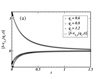
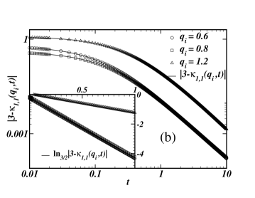
As a test for our numerical algorithm, the result of Eq. (23) was reproduced by a numerical integration, for typical values of $q_{i}$, as shown in Fig 3. The integration was carried out using a method based on distributed approximating functionals Zhang:97 . In all cases, we considered the distribution of Eq. (3) with $b_{q_{i}}(t=0)=1$, as the initial state. The results are represented in different scales, like the linear-linear [Fig. 3(a)] and double logarithm [Fig. 3(b)] ones. However, an elegant way to show that $\kappa_{1,1}(q_{i},t)$ decreases as a $q$-exponential function, with $q_{\rm rel}=3/2$, is by representing the data in terms of the inverse function, i.e., the corresponding $q$-logarithmic function. This is exhibited in the $q$-logarithm-linear plots in the inset of Fig. 3(b), where one observes perfect linear fits, whose slopes give the associated relaxation times, $1/[4(5-3q_{i})]$.

Figure 4: Time evolution of the inflection-point position, $x_{\rm infl}$ (scaled by $\sqrt{t}$), for typical initial $q$-Gaussians, characterized respectively, by $q_{i}=1.2,1.5,\ {\rm and}\ 2.0$ (from top to bottom). The small fluctuations are just a numerical artifact.

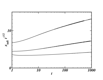
In a recent analytical work it was shown that the diffusion equation, when initialized with a $q$-Gaussian distribution ($1<q_{i}<3$), will asymptotically approach its final solution, i.e., a Gaussian distribution ($q=1$) Anteneodo:06 . Herein, we present a numerical method to investigate how this change occurs for different values of $q_{i}$ within this range. One may see easily that the $q$-Gaussian distributions, defined in Eq. (3), present an inflection point for $q>1$, when represented in a semi-logarithmic plot; the same does not occur for $q\leq 1$. Therefore, one expects that in the transformation process from an initial $q$-Gaussian, characterized by an entropic index $q_{i}>1$, to the asymptotic Gaussian, with $q=1$, such an inflection point should remain at intermediate times, i.e., in the transient regime, and afterwards, it should approach infinity. An example of this effect is shown in the inset of Fig. 2(b), where we exhibit the corresponding time evolution of an initial $q$-Gaussian distribution denoted by $q_{i}=1.25$. Hence, the time evolution of this inflection point may provide some additional information regarding the process of approach to the Gaussian distribution, and in particular, in the cases $q_{i}>7/5$, for which the kurtosis of Eq. (23) is not defined. Let us herein denote the position of the inflection point by $x_{\rm infl}$; we analyze the time evolution of the rescaled quantity, $(x_{\rm infl}/\sqrt{t})$, in order to measure the time evolution of the inflection point taking off the usual spreading effect of the distribution during the diffusion process. We have followed the time evolution of $(x_{\rm infl}/\sqrt{t})$ for different initial values $q_{i}$, as shown in Fig. 4. Within the time interval feasible for computational purposes, we have noticed that $(x_{\rm infl}/\sqrt{t})$ always increases in time and hopefully diverges, in agreement with the results of Ref. Anteneodo:06 . However, one notices that for higher values of $q_{i}$, such an increase occurs very slowly, and in particular, the case $q_{i}=2$ suggests that the transformation to the asymptotic Gaussian distribution should take place at a very long time. The fact that a single diffusing particle, described in terms of a linear equation [Eq. (1)], may take a very long time to reach its asymptotic-diffusing regime, supports the result found in some Hamiltonian systems, described by a set of $N$ coupled differential equations, for which, given some initial conditions, the final equilibrium may never be reached in the thermodynamic limit ($N\rightarrow\infty$) LatoraRuffo:98 ; Anteneodo:98 ; Moyano:06 ; Pluchino:07 ; Pluchino:08 ; nobretsallis:03 ; nobretsallis:04 .

V General case: ${q}\neq 1$

In this section we analyze the general case $q\neq 1$, which corresponds to the nonlinear porous-medium equation. The investigation of the solutions of such equation was done through a numerical integration of Eq. (1), using the same method applied in the previous section. Therefore, we followed the time evolution of the kurtosis, which starts from $\kappa_{\bar{r},q}(q_{i},0)$ [Eq. (11)] and will evolve towards its asymptotic limit, $\kappa_{\bar{r},q}(q)$ [Eq. (12)]. In particular, we will search for the relaxation law associated with $|\kappa_{\bar{r},q}(q)-\kappa_{\bar{r},q}(q_{i},t)|$.

Figure 5: Time evolution of the absolute values of the differences between the kurtosis at their initial and final values, $\kappa_{\bar{r},q}(q_{i},t)$ [Eq. (11)] and $\kappa_{\bar{r},q}(q)$ [Eq. (12)], respectively, for typical initial and final $q$-Gaussians. (a) $q=3/4$ and several initial values of $q_{i}$; the full straight line corresponds to the power-law decay $t^{-5/2}$. (b) $q=5/4$ and several initial values of $q_{i}$; the full straight line corresponds to the power-law decay $t^{-3/2}$. (c) The data of (a) is represented in a $\log_{7/5}$ scale. (d) The data of (b) is represented in a $\log_{5/3}$ scale.

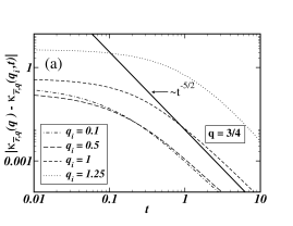
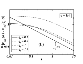
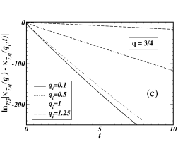
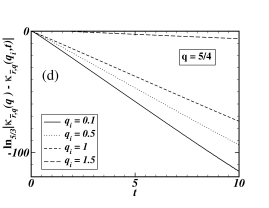
In Fig. 5 we exhibit the quantity $|\kappa_{\bar{r},q}(q)-\kappa_{\bar{r},q}(q_{i},t)|$ for two typical final $q$-Gaussians, namely $q=3/4$ and $q=5/4$, starting the numerical procedure with different initial $q$-Gaussians. Similarly to what happened in the previous section, our numerical investigation yields, in both cases, that the kurtosis relaxes to the corresponding final values, $\kappa_{\bar{r},q}(q)=2.34797...$ $(q=3/4)$ and $\kappa_{\bar{r},q}(q)=3.81717...$ $(q=5/4)$, according to $q$-exponentials, whose relaxation index $q_{\rm rel}$ depends only on $q$. The full straight lines in Figs. 5(a) and 5(b) correspond to the power-law decays, $t^{-5/2}$ and $t^{-3/2}$, which are associated with $q$-exponentials characterized by the relaxation indexes, $q_{\rm rel}=7/5$ (for $q=3/4$) and $q_{\rm rel}=5/3$ (for $q=5/4$), respectively. Taking into account the results obtained in the previous section as well, i.e., a relaxation following a $q$-exponential with $q_{\rm rel}=3/2$ (for $q=1$), we propose a general form for the relaxation of the kurtosis,

$$|\kappa_{\bar{r},q}(q)-\kappa_{\bar{r},q}(q_{i},t)|=A(q_{i},q)\left[1+(1-q_{\rm rel})b^{2}f(q_{i},q)t\right]^{1/(1-q_{\rm rel})}~{},$$ (24)

where the index $q_{\rm rel}$ associated with the $q$-exponential relaxation process depends only on the index $q$, characteristic of the asymptotic $q$-Gaussian distribution, and that it appears to follow the heuristic relation,

$$q_{\rm rel}(q)=\frac{2q-5}{2q-4}~{}.$$ (25)

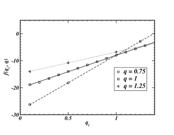
The coefficient $A(q_{i},q)$ that appears in Eq. (24) should satisfy $A(q,q)=0$, in such a way that starting the numerical integration procedure with the exact solution of Eq. (1), the kurtosis should not change in time, i.e., the initial distribution remains stable for all times. The argument of the $q$-exponential, $f(q_{i},q)$, should recover the particular case $q=1$, calculated analytically, $f(q_{i},1)=-4(5-3q_{i})$ [cf. Eq. (23)]. This argument was estimated numerically for typical values of $q\neq 1$, as shown in Fig. 6, and our results suggest a simple (essentially linear) general form, $f(q_{i},q)=a(q)+b(q)q_{i}$.

Figure 6: The argument $f(q_{i},q)$ of the $q$-exponential characterizing the relaxation of the kurtosis, from an initial $q$-Gaussian (index $q_{i}$) to an asymptotic $q$-Gaussian (index $q$), as defined in Eq. (24), is exhibited as a function of $q_{i}$, for different values of $q$. In the case $q=1$, the points (represented by squares) were computed numerically, whereas the full line corresponds to the analytical result. In the case $q=0.75$ ($q=1.25$) the points were computed numerically, and the straight dashed (dotted) line corresponds to a linear fit.

VI Conclusions

We have analized, using both analytical and numerical approaches, the stability of $q$-Gaussian distributions as particular solutions of the porous-medium equation. This was done by investigating the relaxation towards the final, asymptotic $q$-Gaussian solution, characterized by an index $q_{f}$, when considering as an initial distribution a $q$-Gaussian, specified by an index $q_{i}$. By following the time evolution of the kurtosis (defined for $q_{i}<7/5$, but always finite in the asymptotic limit, $t\gg 1$), we have found evidence that such a relaxation process follows a $q$-exponential function, characterized by a relaxation index $q_{\rm rel}(q)$. Therefore, in principle, the problem considered may be formulated in terms of four indexes: (i) the index $q$ defined by the porous-medium equation; (ii) $q_{i}$, associated with the initial $q$-Gaussian distribution; (iii) $q_{f}$, associated with the final $q$-Gaussian distribution; (iv) $q_{\rm rel}$, related to the $q$-exponential of the relaxation towards the asymptotic distribution. Since we have found no evidence of $q_{f}\neq q$, we assumed that $q_{f}\equiv q$; this supposition is also supported by a recent analytical approach of the asymptotic behavior of the linear diffusion equation Anteneodo:06 . Accordingly, our study was restricted to three indexes, namely, $q,\,q_{i}$, and $q_{\rm rel}$.

In the definition of this kurtosis, the powers ($s$ and $r$) that appear in the probability distributions of the second and fourth generalized moments were chosen conveniently in order to yield a finite kurtosis in the limit $t\gg 1$; although these choices are arbitrary, we expect that other alternatives (e.g., those used in Ref. Estrada:08 ) should not change the present results qualitatively. By using a numerical approach based on the evolution of the inflection point that appears in a semi-logarithmic plot of a $q$-Gaussian with $q>1$, we have observed that in some cases, an initial infinite-variance distribution ($q_{i}\geq 5/3$) may take a very long time to be transformed into a finite-variance one ($q<5/3$). In particular, considering the linear diffusion equation, we have shown through this method that an infinite-variance distribution ($q_{i}\geq 5/3$) evolves very slowly in time towards the asymptotic Gaussian distribution. The fact that a single diffusing particle, described in terms of a linear equation, may take a very long time to reach its asymptotic-diffusing regime, supports the existence a metastable state found in some highly-interacting Hamiltonian systems, described by a set of $N$ coupled linear differential equations, whose duration diverges in the thermodynamic limit ($N\rightarrow\infty$). Moreover, for a finite (but sufficiently large) $N$, it has been found recently that the angles described by the infinite-range-interaction XY rotator model follow a distribution in the long-time-limit (i.e., in the limit for which its kinetic temperature coincides with the one of the BG canonical ensemble) that is well-fitted by a $q$-Gaussian, with $q\approx 1.5$ Moyano:06 . This suggests that in such Hamiltonian models the BG equilibrium state is approached through different steps, one of them being the attainment of the equilibrium temperature; in the simpler system considered herein, the approach to the final, asymptotic solution, follows a relaxation behavior that may be also very slow in some cases.