Wormholes and trumpets:
the Schwarzschild spacetime for the moving-puncture generation

Abstract

We expand upon our previous analysis of numerical moving-puncture simulations of the Schwarzschild spacetime. We present a derivation of the family of analytic stationary 1+log foliations of the Schwarzschild solution, and outline a transformation to isotropic-like coordinates. We discuss in detail the numerical evolution of standard Schwarzschild puncture data, and the new time-independent 1+log data. Finally, we demonstrate that the moving-puncture method can locate the appropriate stationary geometry in a robust manner when a numerical code alternates between two forms of 1+log slicing during a simulation.

I Introduction

The binary black hole problem is a cornerstone problem in gravitational theory: solving for the inspiral and merger of two black holes in full general relativity connects the theory’s strong-field regime with astrophysics, and connects issues with the mathematical understanding of the theory with the emerging field of gravitational-wave astronomy. Solutions of the binary black hole problem require numerical simulations, but stable, long-term numerical evolutions of orbiting black-hole binaries eluded researchers for four decades. However, after a number of insights and technical developments two independent methods Pretorius (2005); Campanelli et al. (2006a); Baker et al. (2006a) were shown in 2005 to allow simulations of the last orbits, merger and ringdown of an equal-mass nonspinning binary. One of these, the “moving puncture method” Campanelli et al. (2006a); Baker et al. (2006a), was quickly adopted by many research groups and has since been applied to many, more general, scenarios: unequal-mass binaries Herrmann et al. (2007a); Baker et al. (2006b); González et al. (2007a); Buonanno et al. (2007), spinning binaries Campanelli et al. (2006b, c, 2007a, 2007b); Herrmann et al. (2007b, c); González et al. (2007b); Hannam et al. (2007a); Brügmann et al. (2007); Koppitz et al. (2007); Pollney et al. (2007); Rezzolla et al. (2007a, b); Hannam et al. (2007b); Dain et al. (2008); Baker et al. (2008), three-black-hole spacetimes Campanelli et al. (2007c); Lousto and Zlochower (2008) and long simulations of (so far) up to ten orbits Baker et al. (2006c); Hannam et al. (2008); Husa et al. (2007a, b).

At the technical level, the moving-puncture method consists of a seemingly small modification of the earlier “fixed puncture” method Brügmann (1999); Alcubierre et al. (2003a). However, in Hannam et al. (2007c) (which we will refer to as Paper I), we found that the numerical slices behave in a way radically different from what was observed in previous fixed-puncture evolutions, and indeed in all previous numerical simulations of black-hole spacetimes. We developed a geometrical picture of the behavior of moving-puncture simulations, and our results suggested a new paradigm for black-hole evolutions, centered around manifestly stationary representations of black-hole spacetimes and “asymptotically cylindrical” slices. This led to further investigations in Hannam et al. (2007d); Brown (2008); Garfinkle et al. (2007). In this paper we expand and discuss in more depth the results of Paper I, with particular reference to the asymptotics of the initial and final states of a moving-puncture simulation

The initial data in a typical moving-puncture simulation represent black holes using a wormhole topology: as we follow the coordinates toward one of the black holes, we do not reach the black hole’s singularity but instead pass through a wormhole to another exterior space, and eventually find ourselves once again in an asymptotically flat region. Data for $N$ black holes can consist of $N+1$ asymptotically flat regions connected by $N$ wormholes. In the puncture approach to constructing initial data Beig and O’Murchadha (1994); Beig and Husa (1994); Brandt and Brügmann (1997); Dain and Friedrich (2001) each “extra” asymptotically flat region is compactified so that its spatial infinity is transformed to a single point (“puncture”), and the entire $N+1$-wormhole topology can be represented in a single three-dimensional space, $\mathbb{R}^{3}$. All of the black-hole singularities are conveniently avoided in this construction, and there is no need to “excise” any region when these data are used in a numerical simulation.

This use of nontrivial topology to enforce the presence of horizons can be regarded as a mere trick to conveniently construct black-hole initial data. It comes at the expense of using the entire Kruskal extension to the Schwarzschild spacetime, part of which has no physical relevance in typical numerical evolutions. Our analysis suggests that a similar trick could be used to construct initial data that leave out most of the unphysical region; we will later refer to these as “trumpet” data.

Standard puncture data are smooth over the entire space, except for a scalar function, the conformal factor $\psi$, which diverges as $1/r$ near each puncture. One of the two innovations of the moving-puncture method was that it provides a method to stably evolve the conformal factor. In addition, the method uses gauge conditions (variants of “1+log” slicing for the lapse function Bona et al. (1995) and $\tilde{\Gamma}$-freezing for the shift vector Alcubierre et al. (2001); Alcubierre et al. (2003a)) that allow the punctures to move across the numerical grid. The result is that the punctures orbit each other and spiral inwards, as if the black holes were being represented by point particles, and the plots of the “puncture tracks” shown in many papers easily match our intuitive picture of objects in orbit (see, for example, Campanelli et al. (2006a); Baker et al. (2006a, c); Husa et al. (2007a)). Of course, the orbiting punctures are not point particles, they are the asymptotic infinities of wormholes, or at least they were in the initial data. Are these two extra copies of an asymptotically flat region of spacetime orbiting each other on the numerical grid? The answer turns out to be No, as we explain below.

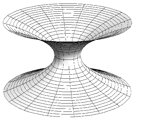
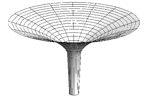
In Paper I we studied moving-puncture simulations of a Schwarzschild black hole, and found that the numerical points quickly leave the extra copy of the exterior space. Where the points near the puncture originally approached a second asymptotically flat end, after a short time the grid points instead asymptote to an infinitely long “cylinder” with radius $R_{0}=1.31M$. In addition, we solved the spherically symmetric Einstein equations for a stationary 1+log-sliced spacetime (see also Buchman and Bardeen (2005)), and found that the one solution with a lapse function that is non-negative everywhere agrees with that found by the numerical code. In other words, there is one regular stationary 1+log solution, and the moving-puncture method quickly finds it. Whereas an embedding diagram of the initial data resembles a wormhole, we will refer to that of the late-time slices as a “trumpet”. This terminology becomes clear in Figures 1 and 2.

This seemingly dramatic change in the appearance of the numerical slices is achieved by the gauge conditions. We start with moment-of-time-symmetry initial data for the Schwarzschild solution, choose the initial lapse $\alpha\equiv 1$ and propagate using the 1+log condition. So far the configuration is symmetric across the throat; we will call this “left-right” symmetry to be consistent with standard Kruskal and Penrose diagrams, although we mean symmetry with respect to the upper and lower halves of Figure 1. So: the initial configuration is left-right symmetric, and the slicing condition preserves this symmetry. This means that all the slices of the foliation will also be left-right symmetric and run from one spacelike infinity to the other. As such, there will not be a stationary limiting slice; we will elaborate on this point in Section II. However, at late times a region of the slice to the right (and a corresponding region to the left) is asymptotically stationary. Now we have to consider the effect of the $\tilde{\Gamma}$-driver shift condition. If we use puncture data, this condition generates a very large shift, pointing to the right, near the puncture. This has the effect of dragging all the data points near the puncture into the region of the Schwarzschild solution between the horizons and finally onto the stationary part of the slicing. This happens extremely quickly. The closer the innermost data point is to the puncture, the longer it takes, but it always happens. A description of this phenomenon was also given in Brown (2008).

There exists a true stationary 1+log slice through the Schwarzschild spacetime. This is what we call the “trumpet”. This is asymptotically flat at one end and cylindrical (of radius $R\approx 1.31M$) at the other. The asymptotically stationary part of the wormhole foliation asymptotes to (part of) this trumpet. The closer the data points are to the puncture, the more of the trumpet we will finally see. Further, we will see only the trumpet — there are no longer any grid points on the non-stationary part of the slice, or any of the slice on the left. We may say that the left half of the slice is grossly under-resolved (in fact, it is not resolved at all!), but the nature of the asymptotic 1+log slice is such that a new asymptotics has formed, and the left half of the slice is causally disconnected from the right: the non-resolution of part of the slice no longer concerns us.

An example that closely mimics some of the behaviour described above was found in one of the first ever numerical simulations of a black-hole spacetime, as early as 1973, by Estabrook et al. Estabrook et al. (1973). They evolved the Schwarzschild solution with maximal slicing. The slices were reflection symmetric about a “throat”. At late times the left and right halves looked approximately stationary. In fact the right half was translated to the right by the Killing vector while the left half was dragged to the left. The throat region approximated a cylinder of radius $3M/2$, which grew linearly with time.

Two phenomena associated with their simulations — “collapse of the lapse” and “slice stretching” — were recurring topics in numerical studies of black-hole spacetimes for the next thirty years Smarr and York (1978); Shapiro and Teukolsky (1986); Beig and Murchadha (1998); Reimann (2005). However, what we consider in this context to be the key feature of their result, the formation of a cylindrical asymptotics, received little, if any, attention before the work in Paper I. There we suggested that the existence of a time-independent representation of the foliation consistent with the new asymptotics, which a numerical code can find with the aid of an appropriate shift condition, is one of the keys to the success of the moving-puncture method. We also took the additional intuitive step of realizing that this time-independent representation could be utilized from the outset of a simulation, to allow the construction of fully time-independent trumpet puncture data.

In this paper we extend the analysis that we provided in Paper I. In Section II we discuss standard wormhole puncture data, which cannot be time-independent, and trumpet puncture data, which can. The canonical examples are the maximally sliced solution Estabrook et al. (1973); Reinhardt (1973) and our stationary 1+log solution. Here we provide a simple derivation of the stationary 1+log solution using a height function approach, and illustrate some of its features in a Penrose diagram. We also transform this solution to isotropic coordinates, providing puncture trumpet data that should be time independent in a moving-puncture simulation.

In Section III we present our numerical method. We start with a brief description of the main features of the BSSN/moving-puncture system, and outline a procedure to construct Penrose diagrams from numerical simulations of the Schwarzschild spacetime. Section IV contains the first set of numerical results: a detailed study of a moving-puncture evolution of wormhole puncture initial data. We show how quickly the numerical data approach a trumpet geometry, how they behave during the transition, and check the accuracy with which they approach the analytic stationary solution. It is important to emphasize that although the numerical solution is stationary in the sense of coordinate-independent functions (for example, a plot of $\alpha$ vs $R$ or of $\operatorname{Tr}(K)$ vs $\alpha$), the numerical coordinates may still exhibit some drift.

This is emphasized in Section V, where we evolve the trumpet puncture data produced in Section II. We demonstrate that these are indeed time independent, up to small numerical errors. Furthermore, if we alternate between two variants of 1+log slicing during an evolution, we show that the numerical data can alternate between two stationary solutions, but that some coordinate drift develops in the process. This drift is minimized by choosing $\eta=0$ in the $\tilde{\Gamma}$-driver shift condition.

Finally, we conclude with some remarks about the potential usefulness of trumpet puncture initial data for black-hole binaries, which will be the subject of future work.

II Wormholes and trumpets: analytic treatment

We begin by summarizing our notation and approach, which is based on the standard “3+1” space+time splitting of Einstein’s equations York (1979). We introduce the Schwarzschild metric in Schwarzschild coordinates, progress to isotropic coordinates, which are better adapted to the standard “puncture” method, and then on to a derivation of the “trumpet” solution previously introduced in Paper I. Our focus here is on solutions that are time-independent, because even in the black-hole binary problem we want to choose coordinates that minimize the gauge dynamics; the only dynamics we really want to see in a numerical code are physical dynamics.

II.1 3+1 decomposition and variables

We start by making a space plus time (3+1) decomposition of the spacetime metric,

$$ds^{2}=-\alpha^{2}dt^{2}+\gamma_{ij}(dx^{i}+\beta^{i}dt)(dx^{j}+\beta^{j}dt).$$ (1)

The three-dimensional metric of a $t={\rm const}$ slice is denoted by $\gamma_{ij}$. The lapse function $\alpha$ gives the proper time between the slice at time $t$, and the next slice at time $t+dt$. The shift vector $\beta^{i}$ prescribes how the coordinates shift between the two slices. The complete data on one timeslice are given by $\gamma_{ij}$ and the extrinsic curvature

$$K_{ij}=\frac{1}{2\alpha}(\nabla_{i}\beta_{j}+\nabla_{j}\beta_{i}-\partial_{t}\gamma_{ij}),$$ (2)

where $\nabla_{i}$ denotes covariant differentiation with respect to the spatial metric $\gamma_{ij}$, and we have used the MTW/ADM sign convention Misner et al. (1973); Arnowitt et al. (1962), not that given in Wald Wald (1984). It proves convenient to also split the extrinsic curvature into its trace $K$ and tracefree part $A_{ij}$, i.e.,

$$K_{ij}=A_{ij}+\frac{1}{3}\gamma_{ij}K.$$ (3)

We further decompose these data with respect to a conformal metric, $\tilde{\gamma}_{ij}$, as follows:

$$\gamma_{ij} = \psi^{4}\tilde{\gamma}_{ij},$$ (4)

$$A_{ij} = \psi^{-p}\tilde{A}_{ij},$$ (5)

$$K = \tilde{K},$$ (6)

$$\beta^{i} = {\tilde{\beta}}^{i}.$$ (7)

Note that in the standard conformal decomposition often used to solve the constraint equations York (1979); Choquet-Bruhat and York (1980), one chooses $p=-2$, but for the BSSN decomposition used in the moving-puncture method, $p=4$. Note also that the trace of the extrinsic curvature and the contravariant components of the shift vector are unchanged by the conformal rescaling. The lapse function can also be transformed, but this is not necessary for the present study. We could also have made other choices of the conformal weights, but we are not interested in those here. The complete data on one time slice are $(\gamma_{ij},K_{ij})$, or equivalently $(\psi,\tilde{\gamma}_{ij},\tilde{A}_{ij},K)$.

For the moment we will not worry about the details of the constraint or evolution equations. In this section we will be interested in finding time-independent representations of the Schwarzschild solution, for which the constraint equations are already satisfied, and the time evolution of the data is trivial (i.e., they do not change in time). Although we will make comments about numerical simulations in this section, we will postpone concrete details until Section III, when we study numerically the time development of our data.

II.2 Wormhole puncture data for a Schwarzschild black hole

The Schwarzschild metric in Schwarzschild coordinates is

$$ds^{2}=-fdT^{2}+f^{-1}dR^{2}+R^{2}d\Omega^{2},$$ (8)

where $f=1-2M/R$. Throughout this paper $R$ and $T$ denote the Schwarzschild radial coordinate and Schwarzschild time. The surface $R=2M$ is the event horizon, $R=0$ is a physical singularity, and $R\rightarrow\infty$ is spatial infinity.

Figure 1: Embedding diagram of a two-dimensional slice ($T=\textrm{const.},\theta=\pi/2$) of the extended Schwarzschild solution. The distance to the rotation axis is $R$. A wormhole with a throat at $R=2M$ connects two asymptotically flat ends.

If we make the coordinate transformation $R=\psi^{2}r$, where

$$\psi=1+\frac{M}{2r},$$ (9)

the Schwarzschild metric becomes

$$ds^{2}=-\left(\frac{1-\frac{M}{2r}}{1+\frac{M}{2r}}\right)^{2}dT^{2}+\psi^{4}(dr^{2}+r^{2}d\Omega^{2}).$$ (10)

These are called (quasi or spatially) isotropic coordinates. Topologically, the constant-$T$ slices are $\mathbb{R}_{+}\times\mathbb{S}^{2}\simeq\mathbb{R}^{3}\setminus\{0\}$, while geometrically (measuring proper areas or the Schwarzschild radius $R$) the slices are wormholes. The isotropic $r$ does not reach the physical singularity at $R=0$. For large $r$ we see that $R\rightarrow\infty$, but for small $r$ we see that once again $R\rightarrow\infty$. There is a minimum of $R=2M$ at $r=M/2$. We now have two copies of the space outside the event horizon, $R>2M$, and the two spaces are connected by a wormhole with a throat at $R=2M$ (Figure 1). This wormhole picture of a black hole forms the basis of the initial data used in current moving-puncture black-hole simulations. The point $r=0$, which represents the second asymptotically flat end, is referred to as the puncture.

In terms of the conformal 3+1 quantities introduced earlier, the Schwarzschild metric in isotropic coordinates is

$$\tilde{\gamma}_{ij} = \delta_{ij},$$ (11)

$$\psi = 1+\frac{M}{2r},$$ (12)

$$\tilde{A}_{ij} = 0,$$ (13)

$$K = 0.$$ (14)

The lapse and shift are

$$\alpha = \frac{1-\frac{M}{2r}}{1+\frac{M}{2r}},$$ (15)

$$\beta^{i} = 0.$$ (16)

If we choose (11) – (14) as our initial data, and propagate the data with the lapse (15) and shift (16), then the data will remain unchanged: they are time-independent data.

As trivial as the time development of these data is, it is difficult to reproduce numerically in a standard 3D black-hole evolution code. The reason is that most codes are not stable when the lapse is negative, which it is here for $r<M/2$. In a numerical code we prefer to use a lapse that is always positive, or at least non-negative. Unfortunately, it is not possible to construct a time-independent, maximal slice of Schwarzschild with two asymptotically flat ends and an everywhere non-negative lapse, no matter what shift conditions we employ Hannam et al. (2003); Reimann and Brügmann (2004a, b). Put another way, a maximal- or 1+log-slicing evolution with two asymptotically flat ends and with a non-negative lapse cannot reach a stationary state. We will now see that the way around these earlier results is to give up one of the asymptotically flat ends.

II.3 Trumpet solution — maximal slicing

Figure 2: Embedding diagram of a two-dimensional slice ($t=\textrm{const.},\theta=\pi/2$) of the maximal solution (17) – (20). The distance to the rotation axis is $R$. In contrast to Figure 1 there is only one asymptotically flat end. The other end is an infinitely long cylinder with radius $R_{0}=3M/2$.

Since maximal initial data with two asymptotically flat ends cannot be time independent, we seek an alternative. One alternative is “trumpet” data. Consider the maximal slice of the Schwarzschild spacetime Reinhardt (1973); Estabrook et al. (1973)

$$\gamma_{RR} = \left(1-\frac{2M}{R}+\frac{C^{2}}{R^{4}}\right)^{-1},$$ (17)

$$K^{i}_{j} = {\rm diag}(2C/R^{3},-C/R^{3},-C/R^{3}),$$ (18)

$$\beta^{R} = \frac{\alpha C}{R^{2}},$$ (19)

$$\alpha = \sqrt{1-\frac{2M}{R}+\frac{C^{2}}{R^{4}}},$$ (20)

with $C=3\sqrt{3}M^{2}/4$ and $R\in[1.5M,\infty)$. We see that $\alpha\geq 0$ for this domain, and at $R_{0}=3M/2$ the lapse goes to zero, as does $\beta^{R}$, while the spatial metric diverges as $R\rightarrow R_{0}$, and so the proper distance from $R_{0}$ to any $R>R_{0}$ is infinite. As we approach $R_{0}$ the timeslice becomes an infinitely long cylinder of radius $3M/2$. This behaviour is illustrated in Figure 2 and we will refer to these data as “trumpets”. These data, like (11) – (14) with (15) and (16), are time independent.

With the benefit of hindsight we see that, rather than adopting the wormhole puncture data (11) – (14) for numerical evolutions, we might be better off transforming (17) – (20) to isotropic-like coordinates (such that $r=0$ corresponds to $R=3M/2$), and using those data instead. Such a transformation was calculated numerically in Hannam et al. (2007d), and it was shown that these data can indeed be evolved stably, and are time-independent up to (convergent) numerical errors. An analytic transformation to isotropic coordinates was given in Baumgarte and Naculich (2007).

II.4 Trumpet solution — 1+log slicing

The data (17) – (20) are maximally sliced, $K=0$. In a numerical simulation, we must solve an elliptic equation at each time step to find the appropriate lapse function that maintains maximal slicing (for these data we could assume that the lapse remains constant, but this will not be true in general black-hole simulations). This is computationally expensive (i.e., slow), and it is therefore currently more practical to choose a slicing condition so that the lapse can be calculated from an evolution equation in the same way as all of the other dynamical variables. One such slicing condition is

$$\partial_{t}\alpha=-n\alpha K,$$ (21)

where $n$ is some constant, usually chosen to be $n=2$. We see that if $K=0$, then the lapse does not evolve, and this condition will maintain maximal slicing for our trumpet data. This slicing condition is part of a class of conditions called “1+log” slicing Bona et al. (1995). The condition (21) is actually not a “geometric” slicing condition in the sense that the slicing resulting from this condition also depends on the shift $\beta^{i}$, i.e., on the spatial coordinates Bona et al. (1995); Alcubierre et al. (2003b). Furthermore, in binary simulations it has been found that unphysical gauge modes arise when (21) is used van Meter et al. (2006), and a preferred choice is

$$(\partial_{t}-\beta^{i}\partial_{i})\alpha=-n\alpha K.$$ (22)

This is equivalent to

$$\mathcal{L}_{\hat{n}}\alpha=-nK,$$ (23)

where $\hat{n}$ is the unit timelike normal to the slice and $\mathcal{L}$ is the Lie derivative. For the rest of this article, whenever we refer to 1+log slicing, we will mean (22). We will refer to Eqn. (21) as “asymptotically maximal slicing” because, if it leads to a time-independent geometry, then that geometry will be maximally sliced.

Since the slicing condition (22) has proven rather beneficial in black-hole simulations, we would like to know what the corresponding time-independent Schwarzschild data are. A stationary 1+log solution was found in Paper I. An earlier result on stationary 1+log slices can be found in Buchman and Bardeen (2005), however its exact relation to the present discussion of punctures remains to be understood. Here we will present one (of many possible) derivations of the solution of Paper I.

II.4.1 Height function derivation

We begin with the Schwarzschild metric in Schwarzschild coordinates, Eqn. (8), and introduce a new time variable, $t$, related to Schwarzschild time by a spherically symmetric height function, $h(R)$, as in Malec and Murchadha (2003),

$$t=T-h(R).$$ (24)

The lapse, shift and future-pointing normal vector in the new coordinates are

$$\alpha = \sqrt{\frac{f}{1-f^{2}h^{\prime 2}}},$$ (25)

$$\beta^{R} = \frac{f^{2}h^{\prime}}{f^{2}h^{\prime 2}-1},$$ (26)

$$n_{\mu} = \left(-\alpha,0,0,0\right).$$ (27)

Here again $f=1-2M/R$, and we have introduced the notation $h^{\prime}=\partial h(R)/\partial R$. We note that only the derivative of the height function appears in the new metric.

It is also useful to note that for any stationary spherically symmetric spacetime the extrinsic curvature is given by

$$K_{RR} = \frac{\beta^{\prime}}{\alpha^{2}},$$ (28)

$$K_{\theta\theta} = R\beta,$$ (29)

$$K_{\phi\phi} = R\beta\sin^{2}\theta,$$ (30)

where $\beta=\sqrt{\beta_{i}\beta^{i}}$ and $\beta^{\prime}=\partial\beta/\partial R$, and the trace of the extrinsic curvature $K=K_{i}^{i}$ is given by

$$K=\frac{2\beta}{R}+\beta^{\prime}.$$ (31)

For the Schwarzschild solution we also have the relation

$$\alpha^{2}-\beta^{2}=1-\frac{2M}{R}.$$ (32)

It will simplify the following calculations if we write $h^{\prime}$ in terms of the lapse as

$$h^{\prime}=-\frac{\sqrt{\alpha^{2}-f}}{f\alpha},$$ (33)

and the shift is now written as

$$\beta^{R}=\alpha\sqrt{\alpha^{2}-f},$$ (34)

where we have chosen the sign of the root to give a non-negative shift.

Following Malec and Murchadha (2003), the trace of the extrinsic curvature, $K$, can be written as

$$K = \frac{1}{\sqrt{-g}}\left(\sqrt{-g}n^{\mu}\right)_{,\mu}$$ (35)

$$= \frac{1}{R^{2}}\partial_{R}(R^{2}h^{\prime}f\alpha).$$

In turn, our 1+log gauge condition can be written for a time-independent solution as

$$\beta^{R}\partial_{R}\alpha=n\alpha K.$$ (36)

Combining Equations (35) and (36) and solving for $\alpha^{\prime}$, we arrive at the following first-order differential equation for the lapse,

$$\alpha^{\prime}=-\frac{n(3M-2R+2R\alpha^{2})}{R(R-2M+nR\alpha-R\alpha^{2})}.$$ (37)

The solution of this equation is an implicit equation for the lapse,

$$\frac{n}{2}\left[3\ln R+\ln(2M-R+R\alpha^{2})\right]-\alpha={\rm constant},$$ (38)

or, more conveniently,

$$\alpha^{2}=1-\frac{2M}{R}+\frac{C(n)^{2}e^{2\alpha/n}}{R^{4}}.$$ (39)

We will now determine $C(n)$. The equation (37) is singular when the denominator is zero. We search for a $C(n)$ such that the numerator and denominator are zero at the same point, and the equation remains regular (the singularity in the equation signifies a transition between an elliptic and a hyperbolic problem as discussed in Garfinkle et al. (2007)). The numerator is zero when

$$\alpha=\pm\sqrt{1-\frac{3M}{2R}}.$$ (40)

We want solutions with an everywhere non-negative lapse, so we choose the positive root. Substituting this into the denominator of (37) we find that the denominator is zero for a particular value of $R$,

$$R_{c}=\frac{3n^{2}M+\sqrt{4n^{2}M^{2}+9n^{4}M^{2}}}{4n^{2}},$$ (41)

where we have chosen the positive root to ensure that $R_{c}$ is always positive. This allows us to evaluate the lapse at that point as

$$\alpha^{2}_{c}=\frac{\sqrt{4+9n^{2}}-3n}{\sqrt{4+9n^{2}}+3n}.$$ (42)

The value of the constant $C(n)$ is now given as

$$C^{2}(n)=\frac{(3n+\sqrt{4+9n^{2}})^{3}}{128n^{3}}e^{-2\alpha_{c}/n}.$$ (43)

We now have the 1+log trumpet solution, given by (39) with (42) and (43) for the lapse, from which we calculate $\beta^{R}$ from (34) and $\gamma_{RR}=1/\alpha^{2}$, and the extrinsic curvature is given by (28) – (30).

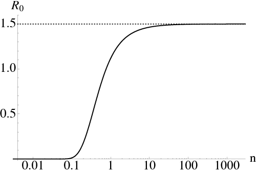
Three special cases of the constant $n$ deserve immediate comment. When $n=2$ we have the form of 1+log slicing commonly used in numerical simulations of black-hole spacetimes. The results presented in Hannam et al. (2007c, d); Brown (2008); Garfinkle et al. (2007) pertain to this case, and we have $R_{c}=1.54M$, $C^{2}(n)=1.55431M^{4}$, and the location of the throat (the smallest real root of (39) with $\alpha=0$) is $R_{0}=1.31241M$. The horizon is located at $\alpha(R=2M)=0.376179$, which differs by over 20% from the common “$\alpha=0.3$” rule-of-thumb estimate of the horizon location.

In the limit $n\rightarrow 0$, Eqn. (36) is degenerate, and two solutions exist. In one, $\beta^{R}=0$, and we recover the standard Schwarzschild metric in Schwarzschild coordinates. In the other, $\partial_{R}\alpha=0$, and so $\alpha=1$ everywhere. As we approach $n\rightarrow 0$, the radius of the throat $R_{0}$ approaches the singularity as $R_{0}\sim e^{-2/(3n)}/(2^{5/3}n)$.

The third case of interest is the limit $n\rightarrow\infty$. Now the only physically meaningful solution is that $K=0$ everywhere, i.e., maximal slicing. We have $C(\infty)=3\sqrt{3}M^{2}/4$, and the radius $R_{c}$ and the throat coincide at $R_{c}=R_{0}=3M/2$. This is the cylindrical maximal slice (17) – (20).

Figure 3: Location of the throat, $R_{0}$, as a function of the coefficient $n$ in the slicing equation (36). In the limit $n\rightarrow\infty$ the stationary slice is maximal and the throat is at $R_{0}=1.5M$, indicated in the figure by a horizontal line. For small values of $n$, the throat approaches the singularity.

II.4.2 Penrose diagrams

One advantage of working in spherical symmetry is that redundant coordinates may be suppressed and we can visualize the way the spacetime is sliced on two-dimensional diagrams, such as the Carter-Penrose diagram.

In order to do this for a given solution (39), we first integrate the height function $h$ using (33) to obtain $T$ for every $R$. The singularity at $R=2M$ can be handled (at least numerically) by introducing a different quantity, such as $e^{-h}$, around the horizon. The undetermined value of $t$ in Eqn. (24), which can be interpreted as the constant of integration, expresses the fact that we do not calculate a single slice but a foliation of the Schwarzschild spacetime. As expected, the slices are related to each other by sliding along the Killing vector field $\partial_{T}$.

From the coordinates $(R,T)$ along one slice we transform to Kruskal coordinates $(u,v)$ by either

$$u = \sqrt{\frac{R}{2M}-1}\>e^{R/(4M)}\cosh\frac{T}{4M},$$ (44)

$$v = \sqrt{\frac{R}{2M}-1}\>e^{R/(4M)}\sinh\frac{T}{4M},$$ (45)

for $R>2M$ or

$$u = \sqrt{1-\frac{R}{2M}}\>e^{R/(4M)}\sinh\frac{T}{4M},$$ (46)

$$v = \sqrt{1-\frac{R}{2M}}\>e^{R/(4M)}\cosh\frac{T}{4M},$$ (47)

for $R<2M$. Compactifying the result via

$$u\pm v=\tan(U\pm V),$$ (48)

where $U$ and $V$ are the abscissa and the ordinate of the Penrose diagram, yields the picture displayed in Figure  4. Note that we chose non-negative shift $\beta^{R}$, which also determines the sign of $h$ (as well as $u$ and $v$ in Eqns. (44) and (45)) . The opposite choice would lead to slices that are mirror images of those in Figure 4, connecting $i_{R}^{+}$ to $i_{L}^{0}$.

\begin{overpic}[width=227.62204pt]{Penanalyt.png} \put(75.0,62.0){$i_{R}^{+}$} \put(24.0,63.0){$i_{L}^{+}$} \put(86.0,48.0){$\mathscr{I}^{+}$} \put(10.0,48.0){$\mathscr{I}^{+}$} \put(8.0,12.0){$\mathscr{I}^{-}$} \put(85.0,12.0){$\mathscr{I}^{-}$} \put(74.0,-2.0){$i^{-}_{R}$} \put(23.0,-2.0){$i^{-}_{L}$} \put(-2.0,33.0){$i_{L}^{0}$} \put(99.0,32.0){$i_{R}^{0}$} \put(33.0,12.0){\begin{rotate}{51.0} $R=2M$ \end{rotate}} \put(55.0,19.0){\begin{rotate}{-51.0} $R=2M$ \end{rotate}} \put(45.0,63.0){$R=0$} \end{overpic}

Figure 4: The Penrose diagram of the slices defined by the stationary solution of the 1+log condition with $n=2$. Every slice approaches $i_{L}^{+}$ along the curve $R=R_{0}\approx 1.31M$ and spatial infinity $i_{R}^{0}$ along a curve of constant $T$. The slices are displayed in time steps of $4M$.

II.4.3 Trumpet data in isotropic coordinates

We have now derived the stationary 1+log solution. In Paper I we compared this solution with the late-time data from moving-puncture evolutions of wormhole puncture data, which we will discuss again in Section III. We would also like to put this solution into isotropic-like coordinates, as was done for the maximal trumpet data in Hannam et al. (2007d); Baumgarte and Naculich (2007). This provides a good test-case for numerical evolution codes, and could be a starting point for generating trumpet data for black-hole binaries.

The implicit nature of the solution (39) makes it difficult to analytically construct the transformation to isotropic coordinates. However, solving (39) for a function $R(\alpha)$ leads to four roots of a fourth order polynomial, which, if chosen appropriately, represent the analytical solution. In this section, $R$ should always be understood as this function of $\alpha$, whereas $\alpha$ becomes the independent variable that parametrizes the spatial dependency. Apart from that our approach is similar to the one used in Baumgarte and Naculich (2007). We note that the $\gamma_{RR}$ component of the stationary 1+log metric can be related to the $\gamma_{rr}$ in isotropic coordinates by

$$\gamma_{RR} = \left(\frac{\partial r}{\partial R}\right)^{2}\gamma_{rr}$$ (49)

$$= \left(\frac{\partial r}{\partial R}\right)^{2}\psi^{4}.$$ (50)

We therefore find that, using $R=\psi^{2}r$ and $\gamma_{RR}=\alpha^{-2}$,

$$\frac{\partial r}{\partial R}=\frac{r}{\alpha R},$$ (51)

and a relation between the isotropic coordinate $r$ and Schwarzschild $R$ may be found by either

$$r = \exp\left(\int^{\alpha}\frac{1}{\bar{\alpha}R}\frac{dR}{d\alpha}(\bar{\alpha})\>d\bar{\alpha}\right),\ \ \ \ \ {\rm or}$$ (52)

$$r = R^{1/\alpha}\exp\left(-\int_{\alpha}^{1}\frac{\ln R}{\bar{\alpha}^{2}}d\bar{\alpha}\right),$$ (53)

where the last equation is obtained by integration by parts and the upper integration limit is chosen such that $r\rightarrow R$ as $\alpha\rightarrow 1$, i.e., towards spatial infinity. Both integrals (52) and (53) diverge as $\alpha\rightarrow 0$, but (52) diverges less strongly, and can be integrated numerically to arbitrarily small $\alpha$ with sufficient accuracy to produce data suitable for a numerical evolution. On the other hand, (53) has the attractive property that as $\alpha\rightarrow 1$ the factor $R^{1/\alpha}$ gives the asymptotic behaviour that we wish. In practice, we choose a point $\alpha_{s}=0.1$, and for $\alpha<\alpha_{s}$ use

$$r(\alpha)=R(\alpha_{s})^{(1/\alpha_{s})}\exp\left[-\int_{\alpha}^{\alpha_{s}}\frac{1}{\bar{\alpha}R(\bar{\alpha})}\frac{dR}{d\alpha}(\bar{\alpha})\>d\bar{\alpha}-C_{0}\right],$$ (54)

where

$$C_{0}=\int_{\alpha_{s}}^{1}\frac{\ln R(\alpha)}{\alpha^{2}}d\alpha.$$ (55)

For $\alpha>\alpha_{s}$ we use

$$r(\alpha)=R(\alpha)^{(1/\alpha)}\exp\left[\int_{\alpha_{s}}^{\alpha}\frac{\ln R(\bar{\alpha})}{\bar{\alpha}^{2}}d\bar{\alpha}-C_{0}\right].$$ (56)

Once we have the solutions $R(\alpha)$ and $r(\alpha)$, we may construct $r(R)$ to whatever accuracy is desired, and then transform our data to isotropic coordinates via

$$\psi = \sqrt{\frac{R}{r}},$$ (57)

$$\beta^{r} = \frac{\partial r}{\partial R}\beta^{R},$$ (58)

$$K_{rr} = \left(\frac{\partial r}{\partial R}\right)^{-2}K_{RR}.$$ (59)

Note that the singularity in the conformal factor is now milder than in the standard puncture case, where $\psi\sim 1/r$, while here

$$\psi(r)=\sqrt{\frac{R(\alpha(r))}{r}}\simeq\sqrt{\frac{R_{0}}{r}}\sim\frac{1}{\sqrt{r}}.$$ (60)

This fact is intuitively expressed in the embedding diagrams in Figures 1 and 2: the expansion of the wormhole geometry as compared to the trumpet geometry leads to a stronger singularity of the conformal factor. Since wormholes and trumpets both allow a representation on $\mathbb{R}^{3}$ where a coordinate singularity at $r=0$ is absorbed in the conformal factor $\psi$, we refer to both cases as punctures.

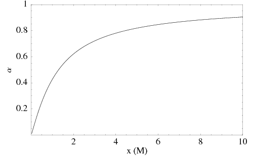
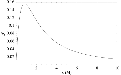
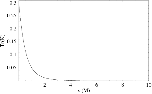
All of the numerical calculations described here were performed with Mathematica, and the data output as tables of physical quantities parametrized by the isotropic coordinate $r$. The data files were then read into our full 3D code Brügmann et al. (2004, 2008), where they were transformed to Cartesian coordinates and interpolated onto the numerical grid. Examples of the resulting data for $\alpha$, $\beta^{x}$ and $K$ are shown in Figure 5. The time independence of these data will be explicitly demonstrated in numerical evolutions in Section V.

Figure 5: The lapse $\alpha$, $x$-component of the shift vector $\beta^{x}$, and $K$ for time-independent 1+log data in isotropic coordinates. The data are shown along the $x$-axis.

III Numerical simulations

We now turn to the numerical evolution of wormhole and trumpet puncture data for the Schwarzschild spacetime. We start with a brief description of the moving-puncture method and our numerical techniques, as well as a summary of our procedure for analyzing our results (including the construction of Penrose diagrams), before finally presenting our numerical results.

III.1 The BSSN/moving-puncture system

The 3+1 decomposition provides evolution equations for the spatial metric $\gamma_{ij}$ and extrinsic curvature $K_{ij}$ York (1979). The BSSN reformulation consists of rewriting the evolution equations in terms of conformally rescaled variables, $\{\psi,\tilde{\gamma}_{ij},\tilde{A}_{ij},K\}$, where we now use $p=4$ in (5), and an additional variable is introduced: $\tilde{\Gamma}^{i}=-\partial_{j}\tilde{\gamma}^{ij}$.

When we deal with puncture data, the conformal factor $\psi$ diverges at each puncture, and this is handled in the moving-puncture modification Campanelli et al. (2006a); Baker et al. (2006a) of the BSSN system by replacing $\psi$ with either the variable $\phi=\ln\psi$ or $\chi=\psi^{-4}$ (or $\chi=\psi^{-2}$ Marronetti et al. (2007)), and one of these quantities is evolved instead. The details of the BSSN system are given in Shibata and Nakamura (1995); Baumgarte and Shapiro (1998). We use the BAM code, and provide details of our implementation of the BSSN/moving-puncture system in Brügmann et al. (2008).

Given evolution equations for the variables $\{\tilde{\gamma}_{ij},\tilde{A}_{ij},K,\tilde{\Gamma}^{i}\}$ and $\phi$ or $\chi$, and some initial data, we also need to choose a lapse and shift during the evolution. We have already discussed the 1+log evolution equations (21) and (22) for the lapse function; the stationary slices for these slicing conditions are given in Section II.4. For the shift vector we use the $\tilde{\Gamma}$-driver condition Alcubierre et al. (2001); Alcubierre et al. (2003a),

$$\partial_{t}\beta^{i} = \frac{3}{4}B^{i},$$ (61)

$$\partial_{t}B^{i} = \partial_{t}\tilde{\Gamma}^{i}-\eta B^{i}.$$ (62)

This shift condition is crucial to the behaviour of the moving-puncture system. In black-hole binary simulations it generates a shift that moves the punctures around the grid on trajectories that match very well the motion that would be seen from infinity Hannam et al. (2007c, 2008). This shift also allows the wormhole puncture data to evolve to the stationary 1+log geometry, as shown in Paper I, and as we will see again in Section IV. As we said in the Introduction, the approach to the “puncture geometry” requires a dramatic stretching of the coordinate representation of the slices. We will illustrate this extreme behaviour in detail in the coming sections, but it can be seen most immediately by calculating the norm of the shift vector, $\beta^{2}=\gamma_{ij}\beta^{i}\beta^{j}$, during the first few $M$ of evolution: although $\beta^{i}$ remains finite, and in fact goes to zero as we approach the puncture, $\beta^{2}$ diverges. This can also be seen analytically Tuite . The wormhole slice is stretched such that all of the numerical points extremely quickly leave the part of the slice that cannot be stationary, and the part of the slice in the second copy of the exterior space, and the points relax onto the stationary 1+log slice. This could not happen with a zero shift, and of course would not happen with an arbitrary shift. There may be a large class of shift conditions that produce the same effect, but the first to be found, and the one that is standard in moving-puncture simulations, is the $\tilde{\Gamma}$-driver condition (61) – (62), and variants.

III.2 Penrose diagrams from numerical data

A convenient way to view the numerical evolution of our data is to represent them in a Penrose diagram. Given the Schwarzschild coordinates $R$ and $T$ of a given point, it is straightforward to calculate the corresponding point on a Penrose diagram. From our numerical data we can easily calculate the Schwarzschild coordinate, $R(r,t)$; see Section IV and Eqn. 73. Each point on the initial slice is at a constant Schwarzschild time $T(r,0)=T_{0}$, which we are free to choose, but $T(r,t)$ is not known. Although a variety of ways to compute an appropriate coordinate representation suggest themselves, it actually turned out to be somewhat tricky to find one that works reliably with our numerical data, see also the discussion in Brown (2007) where the transformation to Kruskal coordinates is implemented. Care has to be taken near the horizon at $R=2M$, and in our case some issues arose at mesh refinement boundaries.

An outline of the procedure that we settled on is as follows. The method is also illustrated in Figure 6. We first choose a numerical point $r_{0}$ far from the black hole (in practice a numerical point that does not pass through the horizon during the evolution). As we have already said, on the initial slice that point has Schwarzschild time $T(r_{0},0)=T_{0}$. We use a differential equation for $\dot{T}=\partial T/\partial t$ to integrate forward in time through our numerical data and produce $T(r_{0},t)$. Then, on each time slice, $t=t_{i}$, we use a second differential equation, this time for $T^{\prime}=\partial T/\partial r$, to integrate across the slice and calculate $T(r,t_{i})$. The equation we use is badly behaved near the horizon, and for a set of five points across the horizon we integrate instead a differential equation for $u^{\prime}=\partial u/\partial r$, where $u$ is the Kruskal coordinate defined by (44) and (46).

\begin{overpic}[width=227.62204pt]{T_integration.png} \put(54.0,22.0){$\int\dot{T}dt$} \put(56.0,42.0){$\int T^{\prime}dr$} \put(35.0,46.5){$\int T^{\prime}dr$} \put(24.0,61.0){$\int u^{\prime}dr$} \put(5.5,31.0){$\int T^{\prime}dr$} \put(43.0,25.0){\begin{rotate}{-70.0} $r=\rm const.$ \end{rotate}} \put(82.0,31.0){\begin{rotate}{-2.0} $t=\rm const.$ \end{rotate}} \end{overpic}

Figure 6: A sketch of the method we use to obtain $T(r,t)$. The lines are drawn from actual data with $r_{0}=3.25M$ for the integration in time and $t=10M$ for the integration in space. Only a subset of the grid points is displayed.

We derive the required differential equations by considering the transformation of the spacetime metric between Schwarzschild and numerical coordinates. A differential equation for $\dot{T}$ can be found using the transformation

$$g_{tt}=\left(\frac{\partial T}{\partial t}\right)^{2}g_{TT}+\left(\frac{\partial R}{\partial t}\right)^{2}g_{RR}.$$ (63)

We therefore find

$$\dot{T}=\left(1-\frac{2M}{R}\right)^{\hskip-3.0pt-1}\sqrt{{\dot{R}}^{2}-\left(1-\frac{2M}{R}\right)g_{tt}}~{}.$$ (64)

This expression is valid for $R>2M$ and $u>0$, and we choose $r_{0}=3.25M$, where this is always true. The metric component $g_{tt}$ is given by $g_{tt}=-(\alpha^{2}-\beta_{i}\beta^{i})$. Using (64) we can integrate the Schwarzschild time along the constant $r_{0}=3.25M$ curve for the duration of the simulation. For the numerical coordinate $r_{0}=3.25M$ we now know $R$ and $T$ throughout the numerical evolution.

A differential equation for $T^{\prime}$ on a slice of constant numerical coordinate time can be found by transforming the spatial part of the metric,

$$\gamma_{rr} = \left(\frac{\partial T}{\partial r}\right)^{\hskip-3.0pt2}g_{TT}+\left(\frac{\partial R}{\partial r}\right)^{\hskip-3.0pt2}g_{RR}$$ (65)

$$\Rightarrow~{}~{}{T^{\prime}}^{2} = \frac{\gamma_{rr}-{R^{\prime}}^{2}g_{RR}}{g_{RR}}$$ (66)

$$= \left(1-\frac{2M}{R}\right)^{\hskip-3.0pt-2}\left[{R^{\prime}}^{2}-\left(1-\frac{2M}{R}\right)\gamma_{rr}\right]~{}~{}.$$ (67)

Note that $R$ and $R^{\prime}$ can be readily computed from the numerical data, since we are dealing with data on one numerical timeslice. In order to integrate (67), we must take a square root and choose the sign such that the slices go smoothly through the horizon, and to define which ends of the computational domain belong to which side of the Penrose diagram. The result is

$$T^{\prime}=-\left(1-\frac{2M}{R}\right)^{\hskip-3.0pt-1}\sqrt{{R^{\prime}}^{2}-\left(1-\frac{2M}{R}\right)\gamma_{rr}}~{}~{}.$$ (68)

Equation (68) is integrated along the entire numerical slice, except at the points near the horizon, where $T^{\prime}$ is singular. We overcome this difficulty by instead integrating the Kruskal coordinate $u$ through five points that cross the horizon. A differential equation for $u^{\prime}$ can be found by transforming the $(r,t)$ coordinates to $(u,R)$:

$$\gamma_{rr}=\left(\frac{\partial u}{\partial r}\right)^{\hskip-3.0pt2}g_{uu}+2\frac{\partial u}{\partial r}\frac{\partial R}{\partial r}g_{uR}+\left(\frac{\partial R}{\partial r}\right)^{\hskip-3.0pt2}g_{RR}.$$ (69)

The metric components $g_{uu}$, $g_{uR}$ and $g_{RR}$ can be written in terms of only $u$ and $R$ by making use of the Schwarzschild metric in Kruskal coordinates, $g_{\mu\nu}^{K}$:

$$v = \sqrt{u^{2}-\left(\frac{R}{2M}-1\right)e^{R/(2M)}}\qquad(v>0),$$ (70)

$$g_{uu} = g_{uu}^{K}+\left(\frac{\partial v}{\partial u}\right)^{\hskip-3.0pt2}g_{vv}^{K}=\left(1-\frac{u^{2}}{v^{2}}\right)\frac{32M^{3}}{R}e^{-R/(2M)},$$

$$g_{uR} = \frac{\partial v}{\partial u}\frac{\partial v}{\partial R}g_{vv}^{K}=\frac{4u}{v^{2}}\frac{1}{M},$$

$$g_{RR} = \left(\frac{\partial v}{\partial R}\right)^{\hskip-3.0pt2}g_{vv}^{K}=-\frac{R}{2M}\frac{1}{v^{2}}e^{R/(2M)}~{}.$$ (71)

Producing an equation for $u^{\prime}$ from (69) once again requires the appropriate choice of sign for a square root. The final result is

$$u^{\prime}=\frac{1}{g_{uu}}\left(-g_{uR}R^{\prime}+\sqrt{\left(g_{uR}R^{\prime}\right)^{2}+g_{uu}\left(\gamma_{rr}-{R^{\prime}}^{2}g_{RR}\right)}\right)~{}~{}.$$ (72)

Once equations (68) and (72) have been integrated along a slice, a constant of integration is chosen to give the value already calculated at $r_{0}=3.25M$ using (64), and a choice of $T_{0}$ for the time on the initial slice.

IV The numerical transition from a wormhole to a trumpet

IV.1 Setup

Simulations were performed with computational grids consisting of eight nested cubical boxes. The boxes are labeled by $l=0,1,\dots,7$. Each box contains $N^{3}$ points, and the grid-spacing in each box is $h_{l}=H/2^{l}$, where $H$ is the grid-spacing of the largest box. We denote $h_{min}=h_{l_{max}}$. The simulations were performed in only one octant of a three-dimensional Cartesian grid (the data in the other octants being easily deduced by exploiting the known spherical symmetry of the Schwarzschild spacetime). The grid points are staggered across the coordinate axes, such that the boundaries of the cubical domain are the six planes defined by $x=h_{min}/2$, $y=h_{min}/2$, $z=h_{min}/2$, $x=X$, $y=Y$ and $z=Z$, with $X=Y=Z=192M$, which define the standard “outer boundary” of the computational domain. Three simulations were performed to make a convergence series, with $N={64,96,128}$, and $H={6M,4M,3M}$, $h_{min}={M/21.33,M/32,M/42.67}$. Note that these grid configurations are the same as used for the single black-hole tests in Brügmann et al. (2008).

The numerical simulations discussed in this section start with the initial data (11) – (14), and initial shift $\beta^{i}=0$ and initial lapse $\alpha=1$. A number of additional simulations were performed with initial lapse $\alpha=\psi^{-2}$ for comparison.

The results of the numerical evolution are shown in Figures 7 to 18. The data for these figures were produced by interpolating numerical data onto the $x$ coordinate axis. The spherical symmetry of the solution allows us to analyze the simulation using these data only. The Schwarzschild radial coordinate can be calculated by relating the numerical spatial metric to the Schwarzschild metric (8). We know that $\gamma_{\theta\theta}=R^{2}$, and because of the spherical symmetry we also have $\gamma_{\theta\theta}=(\partial x^{i}/\partial\theta)(\partial x^{j}/\partial\theta)\gamma_{ij}=(\partial x^{i}/\partial\theta)(\partial x^{j}/\partial\theta)\psi^{4}\tilde{\gamma}_{ij}$. Along the $x$-axis, $\theta=\pi/2$, and so $\partial x/\partial\theta=\partial y/\partial\theta=0$ and $\partial z/\partial\theta=x$, and we have

$$R^{2}|_{y=z=0}=\psi^{4}x^{2}\tilde{\gamma}_{zz}.$$ (73)

IV.2 Early-time behaviour

Figure 7 illustrates the main global feature of the time development of the numerical slices, namely the transition from wormhole to trumpet asymptotics. The upper figure shows the proper distance of a given point from the horizon at $R=2M$ versus that point’s Schwarzschild coordinate $R$. The thick line indicates the $t=0$ data. Initially $R=2M$ is the minimal surface, and the data contain two copies of the space outside the horizon. This is the initial wormhole that we have referred to several times. If we consider a surface of revolution around the proper time axis, we obtain just another version of the standard picture of a spacetime wormhole, as shown earlier in Figure 1. We show the data only up to coordinate $R=10M$; the upper and lower lines in the figure quickly asymptote to $\pm$45 degrees, and do not add extra information to the figure. If we follow the upper line outwards, we move further from the origin (the puncture), and the plot ends at $r=8.25M$. If we follow the lower line outwards, we move closer to the puncture, and in this case the plot ends at $r\approx M/40$. The corresponding picture of $R$ in terms of coordinate $r$ is shown in the lower panels of Figure 7.

Figure 7: The top two figures show the proper separation from the (outer) horizon versus the Schwarzschild coordinate $R$. The left panel shows the slices at $t=0,1,2,3M$, and the right panel shows the slice at $t=50M$. The final numerical slice terminates at $R\approx 1.31M$. The vertical line indicates the horizon at $R=2M$, and the six points represent $x/M=1/40,1/20,1/8,2,5,8$ on each slice. The lower two figures show Schwarzschild $R$ versus numerical $r$ for the same points at the same times. The horizontal lines show $R=2M$ and $R=1.31M$.

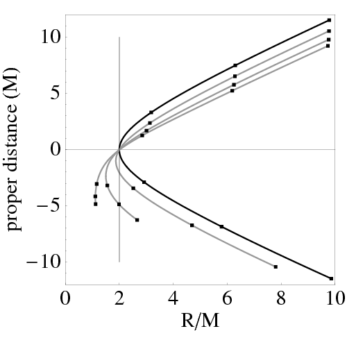
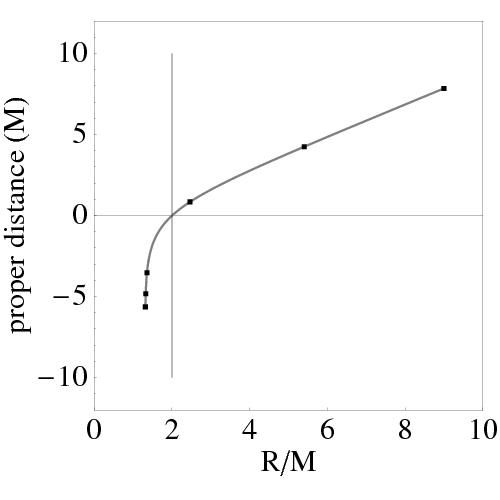
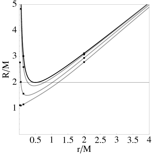
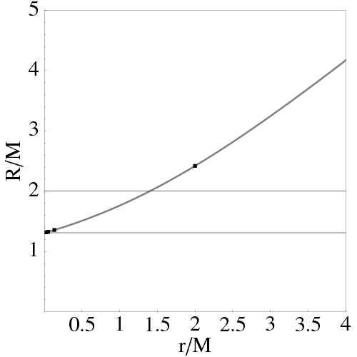
At early times two notable things happen. First, the minimal surface shifts to $R<2M$, and the numerical domain contains two surfaces with $R=2M$, which we will call the “inner” and “outer” horizons. The proper distance in Figure 7 is with respect to the outer horizon. Second, the points in the lower right part of the figure rapidly move to the left. In other words, the Schwarzschild $R$ corresponding to those points rapidly decreases. The numerical points don’t “go” anywhere, of course; they are points on a fixed grid. But their location in the Schwarzschild spacetime does change, and quickly. Within only $3M$ all of the points have passed the inner horizon, and it has ceased to be part of the numerical domain.

At later times ($t>40M$) the points close to the puncture settle at a constant value of $R$, which we will soon see is close to $R_{0}=1.31M$, the location of the throat in the stationary 1+log solution derived in Section II.4. This is shown in the upper right figure. At first sight this does not correspond to the cylindrical asymptotics shown in Figure 2; the “cylinder” looks too short. The reason is that the spatial metric now diverges more slowly as we approach the asymptotic region, and so a point initially “close” to the second asymptotically flat end was a larger proper distance from the outer horizon than it is now that it’s “close” to the cylinder.

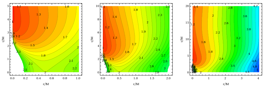
The lower two panels in Figure 7 give a complementary picture. These plot Schwarzschild $R$ versus the numerical coordinate $r$ to illustrate directly how the Schwarzschild $R$ of each grid point changes. The behaviour at early times in terms of $R(r,t)$ is also shown in Figure 8, which shows several contour plots of $R$ (indicated by variations in colour) at different values of coordinate $r$ and time $t$. These figures illustrate many of the main features of the early-time evolution of the wormhole puncture data. We can clearly see that the horizon, initially at $r=M/2$, splits into two copies, and also that values of $R<2M$, which are not present in the initial data, appear as time progresses. We can also see that for larger $r$ the value of $R$ changes very little, although it does decrease for all $r$.

Figure 8: Contour plots showing the behaviour of $R(r,t)$ on the numerical grid for the first $20M$ of a simulation. The axes of the figures give $r$ and $t$ in units of $M$ for three different coordinate ranges. The contour-labels and the colours indicate the value of $R$. We clearly see that $R$ changes rapidly for a given value of the $r$-coordinate for the first few $M$ of evolution before settling down to approximately stationary values at later time. Points with $r>M/2$ accelerate towards the black hole ($R$ decreases) before settling down again at some smaller value of $R$. As the slice moves towards the Schwarzschild singularity, the horizon, initially at $r=M/2$ and $R=2M$, splits into two copies, and values of $R<2M$, which are not present in the initial data, appear as time progresses. The initial slice covers the interior of the black hole from $R=2M$ to $R=+\infty$ for $r=M/2$ to $r=0$. This region is quickly squeezed towards zero extent in $r$, as the lines of constant $R$ in the lower left of the panels indicate. Note that for given $r$, the coordinate motion $R(r,t)$ is not monotonic in $t$, but $R(r,t)$ approaches its asymptotic value via a damped oscillation, see also Figure 11.

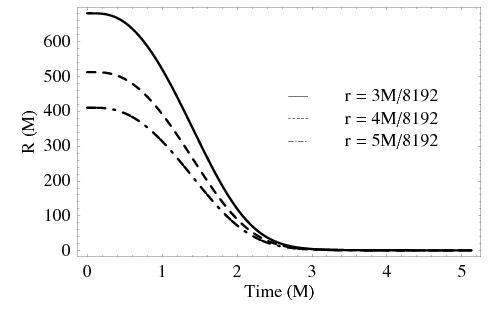
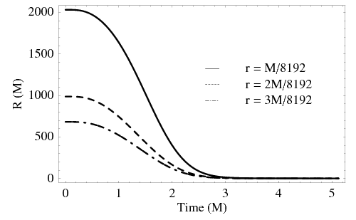
The behaviour of grid points close to the puncture is shown in Figure 9. This plot uses data from a simulation that used extremely high resolution at the puncture: 16 nested boxes, each containing $64^{3}$ points, with a coarsest resolution of $H=4M$ and a finest resolution of $h_{min}=M/8192$; the simulation was run for $t=5M$, in order to obtain the results displayed in Figure 9.

As shown in Paper I, the numerical data become discontinuous across the puncture. This means that finite-difference derivatives (which are used to calculate many quantities in the BSSN evolution) will have even worse discontinuities, and the numerical method cannot converge for points that are within a stencil-width of the puncture, which for the simulations discussed here includes the two grid points closest to the puncture. Fortuitously the nature of the BSSN/moving-puncture system is such that these errors do not seem to propagate out from the puncture, and clean convergence can be seen up to the last few grid points. (This is shown in Figures 2 and 3 of Brügmann et al. (2008).) In the upper panel of Figure 9 we show the time development of $R$ for the third, fourth, and fifth closest points to the puncture of our extremely high-resolution simulation, at $r=\{3,4,5\}M/8192$. Although the points closer to the puncture are not expected to show clean convergence, we see in the lower panel of Figure 9 that they display similar behaviour.

Initially the points in the upper panel are at $R=(1+2M/r)^{2}r=\{684,513,410\}M$. The value does not change significantly for the first $M/2$ of the simulation, but then quickly deceases.

Figure 9: Evolution of $R$ for fixed $r$ for the first $5M$ of an extremely high-resolution simulation. Top panel: the evolution of the third, fourth and fifth closest points to the puncture, at $r=\{3,4,5\}M/8192$, are shown. We do not expect the closest two points to be reliable, due to finite-difference errors across the puncture, although they show similar behaviour, shown in the lower plot.

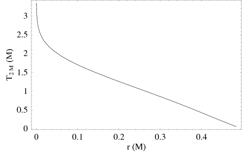
How quickly are our numerical slices flung out of the second copy of the exterior space? Figure 10 shows the time a point takes to reach the inner horizon, parametrized by the point’s isotropic coordinate $r$. The point at $r=M/2$ is at the horizon at $t=0$, and so “reaches” the inner horizon immediately. The time for points with $r<M/2$ to reach the inner horizon appears to grow linearly as we move toward the puncture. Very close to the puncture, however, the time grows logarithmically, and even the closest grid point, at $r=M/8192$ and initially at $R=2049M$, reaches the inner horizon by about $t=3.3M$. A similar result is shown in Brown (2008).

Figure 10: Time for grid points to pass the inner horizon, as a function of coordinate $r$. The innermost grid point is initially at $R=2031M$, and reaches the inner horizon in $T_{2M}=3.35M$.

IV.3 Late-time behaviour and approach to the stationary solution

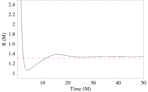
To follow the behaviour of $R(r)$ at later times, we return to our standard convergence series simulations. Figure 11 shows $R$ as a function of time for a grid point at $r=3M/32$. We see that the point, having retreated quickly through the inner horizon, overshoots $R_{0}=1.31M$ (indicated by a dashed line in the figure), before returning and settling to a value just larger than $R_{0}$. We may expect that a point’s Schwarzschild coordinate $R$ can decrease but not increase: a point that falls into the black hole cannot rise back toward the surface, unless the lapse becomes negative and time progresses backward. We will return to this surprising behaviour when we represent the time development of the numerical slices on a Penrose diagram.

Figure 11: The Schwarzschild coordinate $R$ of a point at $r=3M/32$ as a function of time. The point overshoots $R_{0}=1.31M$, indicated by a dashed horizontal line, but for $t>40M$ settles on a value slightly larger than $R_{0}$.

Having described the general behaviour of moving-puncture simulations of Schwarzschild wormhole puncture data, we would like to verify that the numerical solution converges to the analytic one. A natural quantity to look at would be $R$ at the grid points closest to the origin. In Figures 2 and 3 of Brügmann et al. (2008), we have seen that the metric quantities are approximately fourth-order convergent for at least $50M$ of evolution. However, the convergence is not so precise that it is retained in quantities derived from the evolution variables. In particular, $R=\psi^{2}x\sqrt{\tilde{\gamma}_{zz}}$ does not exhibit clean fourth-order convergence, and is not suitable for verifying convergence towards the analytic 1+log geometry.

As an alternative, we look at the value of $\operatorname{Tr}(K)$ on the horizon. Although locating the horizon once again requires an estimation of $R$, the accuracy is much better far from the origin, and a more systematic analysis of the convergence and accuracy of the solution is possible.

Figure 12 shows the value of $\operatorname{Tr}(K)$ at the horizon for simulations that begin with $\alpha=1$ and $\alpha=\psi^{-2}$. In both cases the value relaxes to the analytic result of $K_{H}=0.0668$. Figure 13 shows the convergence of $K_{H}$ for the convergence series described earlier. With a “precollapse” initial lapse of $\psi^{-2}$ we see no sign of convergence at early times, but reasonably clean fourth-order convergence after about $15M$ of evolution. With an initial lapse of $\alpha=1$, we see fourth-order convergence after only a few $M$ of evolution, although the convergence deteriorates at later times.

Figure 12: Time development of $K$ at the horizon, for simulations with initial lapse (a) $\alpha=\psi^{-2}$, and (b) $\alpha=1$.

Figure 13: Convergence of $K$ at the horizon, for simulations with initial lapse (a) $\alpha=\psi^{-2}$, and (b) $\alpha=1$. The $\alpha=\psi^{-2}$ simulations are not convergent at early times, while the $\alpha=1$ simulations lose clean convergence after about $50M$.

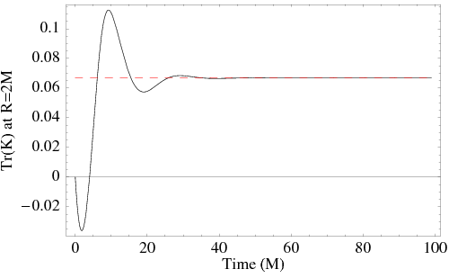
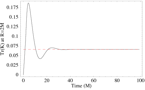
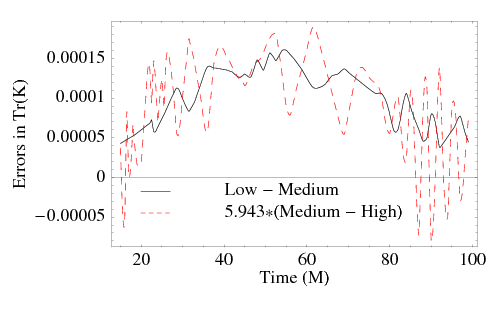
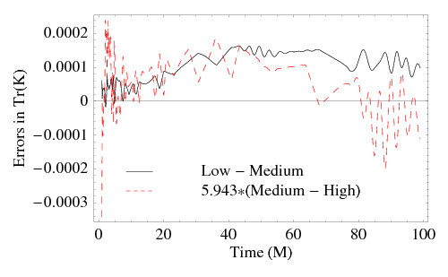
Figure 14 shows the deviation of $K_{H}$ from the analytic value on a logarithmic plot. The values are scaled assuming fourth-order convergence, and we see clearly that the disagreement between the numerical $K_{H}$ and the value for the stationary 1+log slice converge to zero at fourth-order at late times. This provides strong evidence that the numerical slice does indeed approach the analytic stationary slice with high accuracy.

Figure 14: Logarithm of the deviation of $K$ at the horizon from the analytic value $K=0.066811$. The deviations are scaled assuming fourth-order convergence, and the results indicate that $K$ converges to the analytic value with fourth-order accuracy.

IV.4 Penrose diagrams of numerical results

We now represent the time development of the numerical slices on Penrose diagrams, using the technique described in Section III.2. Figure 15 shows such a diagram. The initial conditions are chosen such that the initial data are at $T=0$ and therefore correspond to the horizontal line between $i^{0}_{L}$ and $i^{0}_{R}$. During the evolution, the slices move upwards symmetrically in the diagram. We can clearly see that the points move quickly to the right as the slices move up, and very soon the region near $i^{0}_{L}$ (the second asymptotically flat end) is extremely poorly resolved. In effect the numerical slices lose contact with the second asymptotically flat end and congregate near the cylinder at $R=1.31M$, which is shown by a dashed line.

\begin{overpic}[width=227.62204pt]{Pennum_withshift.png} \put(75.0,62.0){$i_{R}^{+}$} \put(24.0,63.0){$i_{L}^{+}$} \put(86.0,48.0){$\mathscr{I}^{+}$} \put(10.0,48.0){$\mathscr{I}^{+}$} \put(8.0,12.0){$\mathscr{I}^{-}$} \put(85.0,12.0){$\mathscr{I}^{-}$} \put(74.0,-2.0){$i^{-}_{R}$} \put(23.0,-2.0){$i^{-}_{L}$} \put(-2.0,33.0){$i_{L}^{0}$} \put(99.0,32.0){$i_{R}^{0}$} \put(33.0,12.0){\begin{rotate}{51.0} $R=2M$ \end{rotate}} \put(55.0,19.0){\begin{rotate}{-51.0} $R=2M$ \end{rotate}} \put(45.0,63.0){$R=0$} \end{overpic}

Figure 15: Penrose diagram produced from numerical data. We can clearly see the numerical slice retract from the second asymptotically flat end. The times shown are $t/M=0,0.25,0.75,1.25,2.0,2.5,3.5,8$.

We can also see in Figure 15 (and as was also clear in Figure 11), that the slices first penetrate $R_{0}$, before retreating later to a location just outside $R_{0}$. We focus on this behaviour in Figure 16.

Our initial reaction to Figure 11 might be that this is a numerical error: the Schwarzschild $R$ associated with a point can decrease, but it cannot increase unless the lapse is negative and time progresses backwards. We have already seen that the lapse is everywhere non-negative, so this behaviour appears to be contradictory. However, the points can move to larger values of $R$ and move forward in time with the aid of a non-zero shift. Figure 16 illustrates how this is possible.

As a further illustration of this point, consider an arbitrary slice through the Schwarzschild solution. Choose $\alpha=0$ and $\beta^{R}=1$. The data points march along the slice, some with decreasing $R$, some with increasing $R$, depending on the slice we chose. Thus there is no connection between the change of $R$ and the allowed time vectors.

\begin{overpic}[width=170.71652pt]{Pen_mag.png} \put(0.0,23.0){$R_{0}$} \put(0.0,34.0){$R_{b}$} \put(-2.0,48.0){$R_{a}$} \put(39.0,51.0){$\beta^{r}$} \put(60.0,62.0){$R=0$} \put(97.0,62.0){$i^{+}_{R}$} \put(73.0,5.0){\begin{rotate}{67.0} $R=2M$ \end{rotate} } \put(98.0,20.0){$t=t_{a}$} \put(97.0,44.5){$t=t_{b}$} \end{overpic}

Figure 16: A close-up of the region near the cylinder at $R_{0}=1.31M$. Although the time has elapsed from $t_{a}\approx 4.5M$ to $t_{b}=13M$ (with non-negative lapse), $R$ at the innermost gridpoint has increased, $R_{a}<R_{b}$.

It should also be clear that if we were to run our simulation without a shift, then the slices would penetrate $R_{0}$, but would not be able to retreat to $R_{0}$ at later times. This is illustrated in Figure 17, which was produced from a numerical simulation with $\beta^{i}=0$. This behaviour is in direct contrast to what happens in the case of true maximal slicing (where the maximal slicing condition is imposed throughout the evolution, and is not approached only asymptotically, as with the case of the maximal variant of the 1+log condition, (21)), where the slices approach $R_{0}=3M/2$, but cannot pass through it. Maximal slicing is an elliptic condition and thus generates “barriers”, while 1+log slicing is hyperbolic and so no barriers exist.

Note once again that the slices are isometric across the throat, as shown in Figures 15 and 17. The shift only relabels points within the slices and grid points move accordingly, so the figures show identical slices covered by different numerical grids.

\begin{overpic}[width=227.62204pt]{Pennum_withoutshift.png} \put(75.0,62.0){$i_{R}^{+}$} \put(24.0,63.0){$i_{L}^{+}$} \put(86.0,48.0){$\mathscr{I}^{+}$} \put(10.0,48.0){$\mathscr{I}^{+}$} \put(8.0,12.0){$\mathscr{I}^{-}$} \put(85.0,12.0){$\mathscr{I}^{-}$} \put(74.0,-2.0){$i^{-}_{R}$} \put(23.0,-2.0){$i^{-}_{L}$} \put(-2.0,33.0){$i_{L}^{0}$} \put(99.0,32.0){$i_{R}^{0}$} \put(33.0,12.0){\begin{rotate}{51.0} $R=2M$ \end{rotate}} \put(55.0,19.0){\begin{rotate}{-51.0} $R=2M$ \end{rotate}} \put(45.0,63.0){$R=0$} \end{overpic}

Figure 17: Penrose diagram of an evolution identical to that used for Figure 15, except that in this case the shift is zero throughout the evolution and the data points are joined in the plot. We see that the numerical slices no longer retract from the second asymptotically flat end, and now penetrate $R_{0}$, and stay there. The times shown are the same as in Figure 15.

It is difficult to see what happens to the numerical points at late times in Figure 15, because all of the points bunch up in the upper right corner of the diagram. We can change this by choosing $T<0$ for the initial slice when constructing the diagram. Figure 18 shows the slices at numerical times $t=30,37.25,40,50$M, with the initial time chosen as Schwarzschild time $T_{0}=-40$M. We see clearly that the slices approach the cylinder at $R=1.31M$. In addition the figure shows the analytic solution evaluated at the same times, and we see that the numerical points lie perfectly on top of the analytic solution, and that since we have reached the stationary slice, the numerical and Schwarzschild times coincide.

\begin{overpic}[width=227.62204pt]{Pen_late.png} \put(75.0,62.0){$i_{R}^{+}$} \put(24.0,63.0){$i_{L}^{+}$} \put(86.0,48.0){$\mathscr{I}^{+}$} \put(10.0,48.0){$\mathscr{I}^{+}$} \put(8.0,12.0){$\mathscr{I}^{-}$} \put(85.0,12.0){$\mathscr{I}^{-}$} \put(74.0,-2.0){$i^{-}_{R}$} \put(23.0,-2.0){$i^{-}_{L}$} \put(-2.0,33.0){$i_{L}^{0}$} \put(99.0,32.0){$i_{R}^{0}$} \put(33.0,12.0){\begin{rotate}{51.0} $R=2M$ \end{rotate}} \put(55.0,19.0){\begin{rotate}{-51.0} $R=2M$ \end{rotate}} \put(45.0,63.0){$R=0$} \end{overpic}

Figure 18: The numerical data at Schwarzschild times $t=30,37.25,40,50$M, with the initial time chosen as $T_{0}=-40$M. The analytic solution, evaluated at the same times, is shown by a solid grey line. We see that the numerical points lie perfectly on the analytic solution.

V Numerical evolution of trumpet initial data

In the previous section we evolved wormhole puncture data with 1+log slicing and the $\tilde{\Gamma}$-driver shift condition, and found that the numerical data quickly evolved from a wormhole to a trumpet geometry. In this section we start with trumpet data. We first show explicitly that they are time-independent (up to numerical errors, which converge to zero with increasing resolution). We then demonstrate that, if we alternate between variants of 1+log slicing during the evolution (in practice (21) and (22)), the numerical slice alternates accordingly between the respective stationary trumpet geometries. This process also allows us to illustrate how the coordinates can drift in these evolutions, while invariant quantities remain unchanged.

V.1 Evolution of time-independent data

If we evolve the stationary 1+log solution in isotropic coordinates, given in Section II.4.3, we expect the data to be time-independent. This is certainly the case when we look at the data by eye: the evolution variables do not appear to change at all.

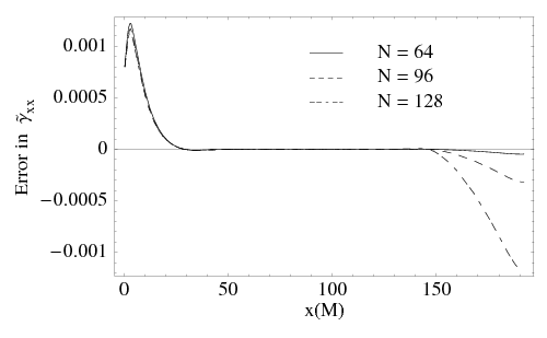
A more systematic test is shown in Figure 19, where we show the error in $\tilde{\gamma}_{xx}$ at $t=50M$. The conformal spatial metric is flat in the stationary data, $\tilde{\gamma}_{ij}=\delta_{ij}$, and so we can calculate the error by simply evaluating $\tilde{\gamma}_{xx}-1$. We see that some error has developed by $t=50M$, and it has a peak at around $x=3M$. The errors are scaled consistent with fourth-order convergence, and we indeed see fourth-order convergence up to around $x=145M$. Since the outer boundary is at $x=192M$, by $t=50M$ lower-order errors from the outer boundary will have propagated to around $x=142M$, and so we do not expect to see fourth-order convergence beyond this point.

Figure 19: The error in $\tilde{\gamma}_{xx}$ (i.e., $\tilde{\gamma}_{xx}-1$) after 50$M$ of evolution of the time-independent trumpet puncture data. The errors for simulations at three resolutions are scaled assuming fourth-order convergence, and we indeed see that the errors converge to zero at fourth-order.

In Figure 20 we show the $L_{2}$ norm of the error in $\tilde{\gamma}_{xx}$ along the $x$-axis as a function of time. The lines are once again scaled assuming fourth-order convergence to zero. We see reasonably clean fourth-order convergence, which appears to deteriorate slightly near the end of the simulation, although by this time lower-order errors from the outer boundary will have contaminated the solution, as is clear in Figure 19.

Figure 20: The $L_{2}$ norm of the error in $\tilde{\gamma}_{xx}$ over the course of the evolution. The errors again converge to zero at fourth-order.

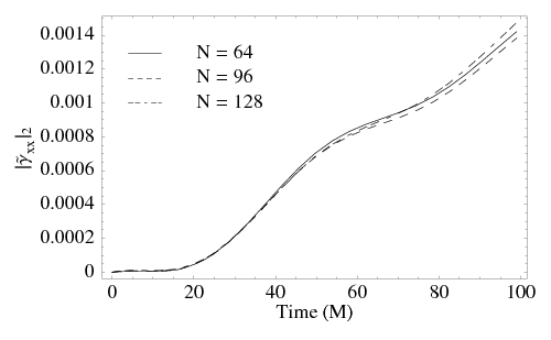
These figures indicate that the data are indeed time independent, up to small numerical errors that converge to zero at the expected rate. Since the analytic value of $\tilde{\gamma}_{xx}$ is unity, we can easily calculate the percentage error from the figures: we see that at $t=50M$ the largest error in $\tilde{\gamma}_{ij}$ is 0.12%, for the lowest-resolution simulation. As such, we see that these data provide an excellent testing ground for the accuracy of a numerical code. This point needs to be emphasized. The moving-puncture approach as used here is currently the most popular method for simulating black-hole binaries. For such a code there is no analytic black-hole solution that can be used to test the code, except for the 1+log and stationary maximal trumpet solutions presented here and in Hannam et al. (2007d); Baumgarte and Naculich (2007). These analytic solutions could be invaluable not only for testing a new code, but also in analysing and reducing the sources of error in current codes.

V.2 Alternating slices

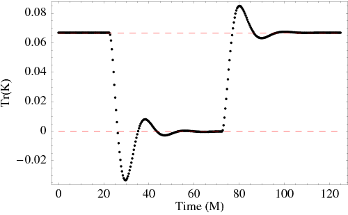
We start with 1+log trumpet data, as in the previous section. We evolve the data for $t=22.5M$, and then switch the slicing evolution equation from (22) to (21), i.e., we change to the slicing condition that asymptotes to maximal slicing. After a further $50M$ of evolution, at $t=72.5M$, we switch back to the original slicing condition, which, assuming robustness of the method, should asymptote back to the stationary 1+log solution.

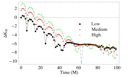
Figure 21 shows the value of $K$ at the horizon for this simulation. The value is $K=0.0668$ on the horizon in the initial data, and remains at this value for the first $22.5M$ of evolution. Then, when the slicing condition changes, $K$ quickly evolves towards $K=0$. Within about $30M$ we have $K\approx 0$. At $t=72.5M$, the slicing condition is changed again, and within another $30M$ the slice has settled back to the stationary 1+log value. Simulations were performed with the same low, medium and high resolutions as the puncture data case in Section IV. At $t=125M$, when the simulations ended, the respective values of $K$ on the horizon were $0.0679,0.0670,0.0669$.

These results illustrate the robustness of the moving-puncture method to locate the appropriate stationary 1+log slice. Potentially more challenging tests have also been performed using excision initial data with the interior filled in, and the method is again seen to be robust Brown et al. (2007); Etienne et al. (2007); Faber et al. (2007).

Figure 21: The value of $K$ at the horizon, for a simulation where the slicing condition alternates between standard 1+log and asymptotically maximal 1+log, Eqns. (36) and (21). The dashed horizontal lines indicate the respective analytic values of $K$ at the horizon.

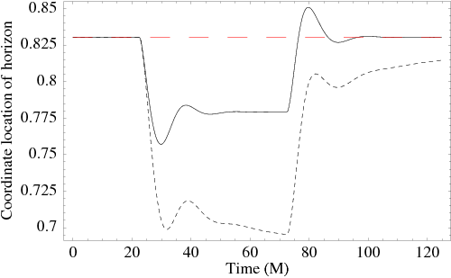
In Figure 22 we show the coordinate distance $r$ of the horizon from the origin. For the stationary 1+log data the horizon is at $r=0.8304M$, and deviates by no more than $0.0014$ % in the first $22M$ of evolution in the highest-resolution simulation. When the slicing condition is switched to asymptotically maximal 1+log, and then back to standard 1+log, we see that the horizon does not return to its original position, at least not on the same time scale as the geometry returns to the stationary 1+log geometry. (See the dashed line in the figure.) This illustrates that, although the numerical slices quickly approach a stationary geometry, the coordinates may still drift. This effect is at least partially due to the damping parameter $\eta$ in the $\tilde{\Gamma}$-driver shift condition. If we repeat the simulation with $\eta=0$, we produce the solid line in Figure 22: now the horizon location returns to its original location to a comparable accuracy that coordinate-invariant quantities return to the stationary 1+log solution.

Figure 22: The coordinate location the horizon, for two simulations with an alternating slicing condition. The dashed line is for a simulation with the standard choice of $\eta=2/M$. The solid line is for a simulation with $\eta=0$. In this case, the horizon location almost returns to its original value when the solution returns to the 1+log stationary geometry.

VI Discussion

VI.1 Setting wormholes and trumpets in motion

One of the directions for future work suggested by our results (and already proposed in Paper I) is the construction of trumpet (as opposed to wormhole) initial data for black-hole binaries.

Trumpet black-hole binary initial data would have the advantage that our numerical code would not need to evolve the fast transition from wormholes to trumpets. In addition, current binary puncture initial data start with zero speed across the numerical grid. When the simulation begins, the 1+log/$\tilde{\Gamma}$-driver gauge conditions both transform the wormholes into trumpets, but also generate an advection component to the shift vector, which moves the trumpets across the grid (Paper I). One could attempt to choose a “better” initial shift, so that the wormholes move from the outset, but if we begin with wormhole puncture data, there is no way to prevent this shift changing nontrivially as the wormholes evolve to trumpets. Although one could produce a “best” initial shift by some trial-and-error process, a more attractive proposal would be to start with trumpet data, and hope to find a procedure to choose an initial shift that imbues the boosted trumpets with their appropriate coordinate speeds. We would then hope that, from the outset, almost all of the evolution of the data would represent the evolution of physical quantities (the black holes’ motions and the evolution of their spins, surface geometry, etc.) and mere gauge evolution would be minimised. This might help reduce the gauge component to the black-hole motion seen in, for example, the first few hundred $M$ of evolution in Figure 18 in Hannam et al. (2008). Further, and more practically, we would hope that such data would reduce the initial noise in wave quantities (for example, Figures 1, 2, 4 and 6 in Hannam et al. (2008)).

Before we become too optimistic, however, we should emphasize that the bulk of the initial noise in most numerical simulations probably comes from the burst of junk radiation present in the initial data. For example, the excision data evolved in Boyle et al. (2007) already have most of the properties we have just advertised: the gauge is not expected to evolve significantly in the early stages of the simulation, and the initial shift is precisely that which should cause the black holes to follow a quasi-circular inspiral. As we would hope, the black-hole motion is indeed smooth from the outset. Nonetheless, noise still reduces the accuracy of some wave quantities at early times (see, for example, Figure 7 of Boyle et al. (2007)), and the most likely culprit is the junk radiation, which has a similar magnitude to that in moving-puncture simulations. We expect that the ideal initial data for moving-puncture simulations would produce minimal junk radiation and be in trumpet form.

VI.2 Summary

We have extended the analysis of the behaviour of the analytical and numerical slices in moving-puncture simulations of the Schwarzschild spacetime that we began in Paper I. For a general form of the 1+log slicing condition (36) we have derived the stationary Schwarzschild trumpet solution: the slice extends from spatial infinity to an infinitely long cylinder, or trumpet, with a throat at some finite radius $R_{0}$. When the parameter $n$ in this condition is set to $n=2$, we obtain the solution given in Paper I with $R_{0}=1.31M$. In the limit $n\rightarrow\infty$ we recover the maximal trumpet solution Estabrook et al. (1973); Reinhardt (1973), with $R_{0}=1.5M$.

For a given choice of the 1+log slicing condition, there is a unique regular stationary solution. In numerical simulations that apply the moving-puncture technique to wormhole puncture Schwarzschild initial data, and use the $\tilde{\Gamma}$-driver shift condition, the numerical slice quickly evolves to the stationary slice. This cannot happen to the analytic slice: this must remain connected to the two asymptotically flat ends in the wormhole data. It also cannot happen with numerical data if the shift is zero. However, the $\tilde{\Gamma}$-driver shift condition generates a shift that stretches the numerical slice such that all of the numerical points extremely quickly move onto the stationary 1+log slice; the non-stationary part of the slice no longer contains any grid points. The stretching of the slice is so extreme that no matter how many numerical points we place near the puncture (so long as there is no point on the puncture) that point will quickly move onto the stationary slice. Even a grid point initially at $r=M/8192$ and $R\approx 2000M$ on the second copy of the exterior space, passes through $R=2M$ in less than $3.5M$ of evolution, and soon after settles near $R=1.31M$.

An alternative to wormhole puncture data are trumpet puncture data. We have transformed the stationary 1+log solution to isotropic coordinates, and shown that these data are indeed time-independent when evolved, up to small numerical errors. In addition, we have shown that the numerical data can easily change from one stationary geometry to another, if the 1+log condition is changed during the evolution, indicating a certain robustness of the method. Finally, we are able to see clearly that although the data approach a stationary slice, the numerical coordinates may still drift.

The realization that the moving puncture method is really based on trumpet puncture data, and that this type of geometry naturally avoids most of the unphysical regions of spacetime in black hole evolutions, establishes a new paradigm for the numerical evolution of black holes and suggests many directions of possible future research. One of the most promising is the construction of trumpet initial data for black-hole binaries, as discussed above. Additionally, one may use the stationary data to make precise tests of numerical codes, for example to improve treatment of mesh-refinement boundaries and outer boundaries, to determine the resolutions necessary to most accurately resolve black-hole spacetimes, and to explore different gauge choices. The stationary solution also provides an ideal background for mathematical studies of the stability properties of the BSSN/moving-puncture system and other evolution systems, that could even be particularly tailored to evolve trumpet puncture data.