Microcanonical quasi-stationarity of long-range interacting systems
in contact with a heat bath

Abstract

On the basis of analytical results and molecular dynamics simulations we clarify the nonequilibrium dynamics of a long-range interacting system in contact with a heat bath. For small couplings with the bath, we show that the system can first be trapped in a Vlasov quasi-stationary state, then a microcanonical one follows, and finally canonical equilibrium is reached at the bath temperature. We demonstrate that, even out-of-equilibrium, Hamiltonian reservoirs microscopically coupled with the system and Langevin thermostats provide equivalent descriptions. Our identification of the key parameters determining the quasi-stationary lifetimes could be exploited to control experimental systems such as the Free Electron Laser, in the presence of external noise or inherent imperfections.

In recent years, systems characterized by interactions that slowly decay at large distances have considerably attracted the attention of experimental and theoretical physicists. Plasmas, gravitational systems, two-dimensional vortices, wave-matter interaction systems, all fall in this category houches . Of particular interest to what follows is the case of the Free Electron Laser (FEL), a source of coherent radiation which is expected to outperform traditional lasers thanks to the properties of a relativistic-electron lasing medium (see, e.g., fel and references therein). For these systems, the prevalence of long-range interactions over mechanisms acting on short-range scales implies an inefficiency of fast collision processes. This is in contrast with the assumptions underlying Boltzmann’s derivation of the transport equation and brings to the fact that long-range interacting systems get easily stuck in (Vlasov) nonequilibrium quasi-stationary states (QSS) houches ; mukamel ; epjb ; anto ; anto_1 . For instance, the possible observation of QSSs in FEL experiments is predicted on the basis of molecular dynamics simulations of isolated (microcanonical) Hamiltonian systems capturing the essential features of the FEL dynamics barre . From an experimental point of view, it is crucial to recognize if a stable nonequilibrium picture survives in the presence of an external environment (or inherent imperfections) acting on the system baldovin ; bbgky ; choi , and which are the parameters playing a key role in the determination of the QSSs lifetimes. In addition, a basic theoretical issue is whether a stochastic dynamics simulating a thermal bath (TB), e.g., of the Langevin type, reproduces the same nonequilibrium features of a Hamiltonian reservoir microscopically interacting with the long-range system.

While for short-range systems the equivalence between Hamiltonian and Langevin thermostats is well established, the connection between these two different descriptions for the nonequilibrium behavior of a long-range system is less clear, and recent simulations baldovin_1 recovered the same results for the two TBs only at equilibrium. Here we demonstrate that Hamiltonian and Langevin TB provide in fact an equivalent description of the behavior of a paradigmatic long-range system also in nonequilibrium conditions. This is established, both analytically and numerically, analyzing the scaling properties of the QSSs lifetimes. We recast the interaction between the system and a Hamiltonian TB in terms of an equivalent set of generalized Langevin equations. The damping coefficient $\gamma$ determines the timescale $t_{bath}$ for the relaxation to canonical equilibrium, achieved when system and TB share the same temperature. However, even in the presence of TB, correlations due to a slow collisional process determine another timescale $t_{coll}$ (depending on system size $N$) which corresponds to a relaxation to a microcanonical QSS. Thus, for $\gamma$ small enough and $N$ not too large, our main result is the discovery of a novel picture for the transport to equilibrium: On a timescale $t_{dyn}\sim 1$ (in dimensionless units) a violent relaxation drives the system into a Vlasov QSS; Then, on a timescale $t_{coll}\sim N^{\delta}$ (with $\delta\geq 1$) the system reaches a microcanonical QSS; Finally, on a timescale $t_{bath}\sim 1/\gamma$, the system crosses over to canonical (thermal) equilibrium.

Thanks to its appealing (yet non-trivial) simplicity, a system which captured a paradigmatic interest among the researchers is the Hamiltonian Mean Field (HMF) model houches ; epjb ; anto ; anto_1 ; baldovin ; bbgky ; choi , which can be thought as a set of $N$ globally coupled $XY$-spins with Hamiltonian

$$H_{HMF}=\sum_{i=1}^{N}\frac{l_{i}^{2}}{2}+\frac{1}{2N}\sum_{i,j=1}^{N}\left[1-\cos(\theta_{i}-\theta_{j})\right],$$ (1)

where $\theta_{i}\in[0,2\pi)$ are the spin angles and $l_{i}=\dot{\theta}_{i}\in\mathbb{R}$ their angular momenta (velocities). Defining the kinetic temperature $T\equiv\sum_{i=1}^{N}l_{i}^{2}/N$ as twice the specific kinetic energy and the specific magnetization as $m\equiv|\sum_{i=1}^{N}(\cos\theta_{i},\sin\theta_{i})|/N$, one obtains the exact relation $E/N=T/2+(1-m^{2})/2$, where $E$ is the total energy of the system. The free energy of the HMF model can be exactly mapped barre onto that of the Colson-Bonifacio Hamiltonian model for the single-pass FEL colson . In such a context, the variables $l_{i}$’s are interpreted as the phase velocities relative to the center of mass of the $N$ electrons and the $\theta_{i}$’s are the electron phases with respect to the co-propagating wave barre . Despite some dynamical and thermodynamic differencies, analogies can also be found between the HMF model and the behavior of one-dimensional self-gravitating systems miller .

When the HMF model is isolated, in order to determine whether the system truly converges toward statistical equilibrium and the timescale of this relaxation, one must develop an appropriate kinetic theory. This is a classical problem addressed, e.g., in newref and, more recently, in bbgky . From the Liouville equation it is possible to derive the BBGKY hierarchy for the reduced joint probability density functions (PDF) $p_{j}(\theta_{1},\ldots,\theta_{j},\dot{\theta}_{1},\ldots,\dot{\theta}_{j},t)$, with ${j}=1,2,\ldots,N$. In the thermodynamic limit $N\to\infty$, $E/N\sim 1$, and fixed volume $V=2\pi$, the hierarchy can be closed by considering a systematic expansion in powers of $1/N$ of the solutions of the equations bbgky . At the order $1/N$, the distribution function $f=Np_{1}$ satisfies

$$\frac{\partial f}{\partial t}+\dot{\theta}\frac{\partial f}{\partial\theta}-\frac{\partial\phi}{\partial\theta}\frac{\partial f}{\partial\dot{\theta}}=\frac{1}{N}C_{coll}(f),$$ (2)

where $\phi(\theta,t)\equiv-\frac{1}{2\pi}\int_{0}^{2\pi}d\theta^{\prime}\cos(\theta-\theta^{\prime})\int_{-\infty}^{+\infty}d\dot{\theta}\ f(\theta^{\prime},\dot{\theta},t)$. For $N\rightarrow+\infty$, the r.h.s. of Eq. (2) is negligible and we get the Vlasov equation newref . For $N$ finite, $C_{coll}(f)$ is a “collision” operator taking into account correlations between particles bbgky . The scaling in Eq. (2) indicates that “collisions” (more properly correlations) operate on a very slow timescale, of the order $Nt_{dyn}$ or even larger when $C_{coll}(f)=0$, as for a spatially homogeneous one dimensional system bbgky . It is precisely because of the development of correlations that the system reaches, on the “collisional” relaxation time $t_{coll}$, a microcanonical Boltzmann distribution. Since $t_{coll}(N)$ diverges for $N\rightarrow+\infty$ (different scalings, $t_{coll}\sim Nt_{dyn},N^{1.7}t_{dyn},e^{N}t_{dyn}$, have been reported depending on the initial conditions timescale ), the domain of validity of the Vlasov equation is huge. Starting from an out-of-equilibrium initial condition, the Vlasov equation develops a complicated mixing process in the single-particle phase space, leading, in most cases, to a QSS anto_1 ; timescale . This process is called violent relaxation since it takes place on a timescale $t_{dyn}\sim 1$. The QSS is a nonlinearly dynamically stable stationary solution of the Vlasov equation on a coarse-grained scale bbgky . The Vlasov equation admits an infinite number of stationary solutions. The statistical theory of Lynden-Bell lb predicts the “most probable” (most mixed) state epjb ; anto . However, in view of the possible occurrence of incomplete relaxations bbgky ; epjb , there are cases in which the QSSs take forms different from those described by Lynden-Bell’s theory.

Figure 1: Caloric curve of the HMF model (solid line). The dashed line is the prolongation of the ordered phase to subcritical energies. See text for details.

The interaction of the system (1) with a reservoir has been studied in Refs. baldovin and bbgky introducing a Hamiltonian and a Langevin TB, respectively. In the latter case, the dynamics of the system is governed by a set of $N$ coupled stochastic equations:

$$\ddot{\theta}_{i}=F_{i}-\gamma\dot{\theta}_{i}+\sqrt{2\gamma{T}_{b}}\xi_{i}(t),$$ (3)

where $F_{i}\equiv-\frac{1}{N}\sum_{j=1}^{N}\sin(\theta_{i}-\theta_{j})$ is the long-range force experienced by the spin $i$, $\gamma$ is a damping coefficient due to the interaction with the TB, ${T}_{b}$ is the TB temperature, and $\xi_{i}$ is a Gaussian white noise satisfying $\langle\xi_{i}(t)\rangle=0$ and $\langle\xi_{i}(t)\xi_{j}(t^{\prime})\rangle=\delta_{ij}\delta(t-t^{\prime})$. Eqs. (3) define the so-called Brownian Mean Field model bbgky (see also choi ). The evolution of the $N$-body PDF is governed in this case by the Fokker-Planck equation, from which a BBGKY-like hierarchy for the $p_{j}$’s can be derived. In the thermodynamic limit $N\rightarrow+\infty$, $T_{b}\sim 1$, $V=2\pi\sim 1$, the hierarchy can be closed by considering an expansion in powers of $1/N$. It is possible to see bbgky that $p_{2}(\theta_{1},\dot{\theta}_{1},\theta_{2},\dot{\theta}_{2})=p_{1}(\theta_{1},\dot{\theta}_{1})\;p_{1}(\theta_{2},\dot{\theta}_{2})+O(1/N)$. Hence, for $N\rightarrow+\infty$, the equation for $f=Np_{1}$ becomes the mean-field Kramers equation:

$$\frac{\partial f}{\partial t}+\dot{\theta}\frac{\partial f}{\partial\theta}-\frac{\partial\phi}{\partial\theta}\frac{\partial f}{\partial\dot{\theta}}=\gamma\frac{\partial}{\partial\dot{\theta}}\left({T_{b}}\frac{\partial f}{\partial\dot{\theta}}+f\dot{\theta}\right)\equiv\gamma C_{bath}(f).$$ (4)

This equation relaxes to the canonical mean-field Maxwell-Boltzmann distribution $f(\theta,\dot{\theta})=\frac{1}{Z}e^{-(\dot{\theta}^{2}/2+\phi(\theta))/T_{b}}$ [with $\phi(\theta)=\lim_{t\to\infty}\phi(\theta,t)$] on a timescale $t_{bath}\sim 1/\gamma$, independent of $N$. For $\gamma=0$ one recovers the microcanonical situation in which the system is isolated. Correspondingly, the Fokker-Planck equation becomes the Liouville equation and the mean field Kramers equation becomes the Vlasov equation.

Figure 2: (Color online) Time evolution of the magnetization with a Langevin TB. The control parameters $\gamma=10^{-7},5\times 10^{-7},10^{-6}$, $N=500,1000,5000$ satisfy $\gamma\ll 1/N^{1.7}\ll 1$. Plots are averages over at most $10$ runs. The system reaches a Vlasov QSS for $t\sim t_{dyn}\sim 1$, a microcanonical QSS for $t\sim t_{coll}\sim N^{1.7}$ and a canonical equilibrium for $t\sim t_{bath}\sim 1/\gamma$.

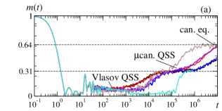
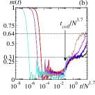
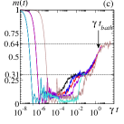
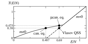
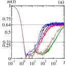
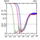
The numerical integration of Eqs. (3) exhibits a very rich transport-to-equilibrium picture baldovin_1 . In this Letter, we show that the key point for understanding the nonequilibrium behavior of the system is the comparison between the timescales $t_{dyn}$, $t_{coll}$ and $t_{bath}$. We specifically analyze the time evolution of the magnetization of the system for simulations with random water bag initial conditions of the form: $p_{1}(\theta,\dot{\theta},0)=\delta(\theta-0)[\vartheta(\dot{\theta}+\overline{l})+\vartheta(\dot{\theta}-\overline{l})]/2\overline{l}$ ($\vartheta$ being the Heaviside step function), where $\overline{l}\simeq 2.03$. We thus have $m(0)=1$, $E(0)/N\simeq 0.69$, and $T(0)=1.38$. These and similar nonequilibrium initial conditions have been largely studied in microcanonical simulations anto_1 ; timescale ; anto and recently discussed in the presence of a TB baldovin ; baldovin_1 . The initial energy of the system is below the critical point $E_{c}/N=3/4$ (see Fig. 1). Microcanonical simulations ($\gamma=0$) display, in a time $t_{dyn}\sim 1$, a violent relaxation process in which the magnetization drops to $m\simeq 0+O(1/\sqrt{N})$ and the temperature to $T\simeq 0.38$. A QSS lasting a time of the order $t_{coll}\sim N^{\delta}$ follows the violent relaxation . After the QSS, the isolated system warms up (at fixed energy) due to finite-size effects, and finally reaches the microcanonical equilibrium state with $T\simeq 0.475$ and $m\simeq 0.31$. At variance, in a relaxation process at fixed temperature $T_{b}=0.38$ (canonical simulations with $\gamma\neq 0$), the system reaches a canonical equilibrium state with $T=T_{b}$, $E/N\simeq 0.487$, and $m\simeq 0.64$ (see again Fig. 1). Hence, if we fix the TB temperature in Eq. (3) at $T_{b}=0.38$, and let $\gamma\to 0$, there is an apparent discontinuity in the final equilibrium value of the magnetization baldovin_1 . Actually, this paradox is solved by the presence of a second QSS which follows the Vlasov one. Indeed, for $t\ll t_{bath}\sim 1/\gamma$ the energy is relatively well conserved. Thus, if $t_{dyn}\ll t_{coll}\ll t_{bath}$ (i.e. $\gamma\ll 1/N^{\delta}\ll 1$), the magnetization of the system relaxes to the microcanonical value $m\simeq 0.31$ on the collisional timescale $t_{coll}\sim N^{\delta}$ (we find $\delta\simeq 1.7$, independently of $\gamma$). This is the reason why we call this second quasi-equilibrium state the “microcanonical QSS”. The equilibrium with the TB, and the consequent value $m\simeq 0.64$, is established only on the much larger timescale $t_{bath}$. On the contrary, for $t_{dyn}\ll t_{bath}\ll t_{coll}$ (i.e. $1/N^{\delta}\ll\gamma\ll 1$), the system first reaches a Vlasov QSS on a timescale $t_{dyn}$, then a canonical equilibrium state with temperature $T=T_{b}$ on a timescale $t_{bath}$, and does not form a microcanonical QSS. We note that in order to see the microcanonical QSS we need a very small noise level: $\gamma\ll 1/N^{\delta}$. There is a further interesting situation, obtained for $t_{bath}\ll t_{dyn}$ (i.e. $\gamma\gg 1$). In this latter case, the system reaches a canonical equilibrium state with temperature $T=T_{b}$, without forming any (Vlasov or microcanonical) QSS. This corresponds to the overdamped (Smoluchowski) regime studied in bbgky . In conclusion, the limits $t\to\infty$, $N\to\infty$, $\gamma\to 0$ do not commute. Depending on the order in which they are taken, the average value of the magnetization can be the Vlasov ($N\rightarrow\infty$ and $\gamma\rightarrow 0$ before $t\rightarrow\infty$), the microcanonical ($\gamma\rightarrow 0$ and $t\rightarrow\infty$ before $N\rightarrow\infty$), or the canonical one ($N\rightarrow\infty$ and $t\rightarrow\infty$ before $\gamma\rightarrow 0$). The simulations reported in Fig. 2 demonstrate these features. In Fig. 2a curves with the same $N$ almost coincide for $t<t_{coll}$; Those with the same $\gamma$ collapse onto each other for $t>t_{coll}$. The presence of a microcanonical QSS following the Vlasov one is particularly evident in the rescaled plots of Figs. 2b,c, which confirm the scaling properties of $t_{coll}$ and $t_{bath}$.

The next step is to establish whether these microcanonical QSSs are an artifact of the mesoscopic stochastic dynamics (3) or if they are still present when we consider a Hamiltonian TB microscopically coupled with the long-range system. In Ref. baldovin a first-neighbors coupled $XY$-spins TB has been introduced,

$$H_{TB}=\sum_{i=1}^{N_{TB}}\frac{{l_{i}^{TB}}^{2}}{2}+\sum_{i=1}^{N_{TB}}\left[1-\cos(\theta_{i+1}^{TB}-\theta_{i}^{TB})\right],$$ (5)

interacting with the HMF model through the potential

$$H_{I}=\epsilon\sum_{i=1}^{N}\sum_{s=1}^{S}\left[1-\cos(\theta_{i}-\theta_{r_{s}(i)}^{TB})\right],$$ (6)

where $r_{s}(i)$ are integer independent random numbers in the interval $[1,N_{TB}]$. Each HMF-spin is in contact with a set of $S$ different TB-spins chosen randomly along the chain, and the coupling constant $\epsilon\geq 0$ determines the interaction strength between system and TB. The conditions baldovin $N_{TB}=N^{2}$ and $S=10^{5}N^{-1/2}$ assure that for large $N$ the interaction, the system, and the TB energies are well separated. Molecular dynamics simulations of the Hamiltonian $H_{HMF}+H_{TB}+H_{I}$ were shown to agree with the Langevin ones at equilibrium baldovin_1 , whereas the presence of QSSs with a lifetime depending on both $\epsilon$ and $N$ (or, equivalently, $S$) has been detected baldovin ; baldovin_1 .

In order to clarify this dependence we study a different Hamiltonian form for the TB and for its interaction with the system, which has the advantage of allowing an explicit analytical analysis. Following the approach outlined by Zwanzig zwanzig for short-range systems, our aim is to recast the Hamiltonian equations of motion in a form similar to Eqs. (3). Hence, we replace Eqs. (5,6) with

$$H_{TB}^{\prime}=\sum_{i=1}^{N_{TB}}\frac{{l_{i}^{TB}}^{2}}{2},\;H_{I}^{\prime}=\epsilon\sum_{i=1}^{N}\sum_{s=1}^{S}\left[\frac{\omega_{r_{s}(i)}}{4}\left(\theta_{i}-\theta_{r_{s}(i)}^{TB}\right)^{2}\right],$$ (7)

respectively, and consider the Hamiltonian $H_{HMF}+H_{TB}^{\prime}+H_{I}^{\prime}$. The TB in Eqs. (7) describes a set of $N_{TB}$ isochronous harmonic oscillators in their canonical coordinates, which interact with the system through a quadratic potential. This quadratic form can be thought as a small-angles expansion of Eq. (6), and again each element of the HMF model interacts with $S$ different TB oscillators. Using for example the Laplace transform and performing then an integration by parts, the Hamiltonian dynamics of the $\theta_{i}$’s becomes

$$\ddot{\theta}_{i}(t)=F_{i}-\int_{0}^{t}dtK(t-\tau)\;\dot{\theta}_{i}(\tau)+\xi^{\prime}(t),$$ (8)

where $K(t)\equiv\epsilon\sum_{i=1}^{S}\omega_{r_{s}(i)}^{2}\cos\left[\sqrt{\epsilon}\;\omega_{r_{s}(i)}t\right]$, and $\xi^{\prime}$ can be written explicitly in terms of the initial conditions .

Figure 3: (Color online) Time evolution of $m$ with the Hamiltonian TB in Eqs. (5,6). In (a,b) the control parameters are $\epsilon=0.1,0.05,0,01$; $N=500,1000,5000$; $S=10^{5}N^{-1/2}$. We found $h\equiv\epsilon^{3/2}S$. In (c) the longer simulations are with $\epsilon=10^{-3},10^{-4}$; $N=500$. Averages are over at most $10$ runs.

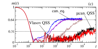
Assuming a random distribution for the initial data, $\xi^{\prime}$ can be regarded as a stochastic term. On the other hand, $K$ is a memory kernel which depends on $\epsilon$, $S$, and on the distribution of the frequencies $\omega_{r_{s}(i)}$. Specifically, when $K$ reduces to a $\delta$-function, Eq. (8) recasts into Eq. (3) with $\gamma=h(\epsilon,S)$, and $h$ a model-dependent function. The form of equations (8) suggests that the relaxation process in the presence of a general Hamiltonian TB should be analogous to that described by the stochastic Langevin Eqs. (3), with the canonical equilibrium established on a timescale $t_{bath}=[h(\epsilon,S)]^{-1}$. In particular, by choosing sufficiently small $\epsilon$’s, the system should exhibit microcanonical QSS also if coupled with a Hamiltonian TB. We verified these conclusions for the Hamiltonian TB in Eqs. (5,6). Figs. 3a,b demonstrate that if we rescale the time by $h(\epsilon,S)=\epsilon^{3/2}S$ indeed the relaxation time to the thermal equilibrium obtained for different $\epsilon$’s and $S$’s collapse onto the same value. Moreover, for $\epsilon\leq 10^{-3}$ microcanonical QSSs clearly appear (Fig. 3c).

In summary, we have shown that the nonequilibrium dynamics of a paradigmatic long-range system which can be mapped onto the one describing the single-pass FEL is characterized by the three timescales $t_{dyn}\sim 1$, $t_{coll}\sim N^{\delta}$, $t_{bath}\sim 1/\gamma$. By acting on the initial conditions, on the system size $N$, or on the coupling with the heat bath $\gamma$, one can conceive experiments in which the system is either in equilibrium with the bath or in a quasi-equilibrium state with a dynamical temperature which is different from the temperature of the thermal environment. This situation could inspire interesting applications and provides a control on the imperfections influencing a FEL and other long-range systems.

References

- (1) Dynamics and thermodynamics of systems with long range interactions, eds T. Dauxois et al., Lect. Notes Phys. 602 (Springer, 2002); Dynamics and Thermodynamics of Systems with Long-range Interactions: Theory and Experiments, eds A. Campa et al., AIP Conf. Proc. 970 (AIP, 2008).
- (2) E. Plönjes et al., Phys. World 16(7), 33 (2003); S. Milton et al., Science 292, 2037 (2001); E. Allaria and G. De Ninno, Phys. Rev. Lett. 99, 018801 (2007).
- (3) D. Mukamel et al., Phys. Rev. Lett. 95, 240604 (2005).
- (4) P.H. Chavanis, Eur. Phys. J. B 53, 487 (2006).
- (5) A. Antoniazzi et al. Phys. Rev. E 75, 011112 (2007).
- (6) A. Antoniazzi et al., Phys. Rev. Lett. 98, 150602 (2007); A. Antoniazzi et al., Phys. Rev. Lett. 99, 040601 (2007).
- (7) J. Barré et al., Phys. Rev. E 69, 045501(R) (2004); J. Barré et al., J. Stat. Phys. 119, 677 (2005).
- (8) F. Baldovin and E. Orlandini, Phys. Rev. Lett. 96, 240602 (2006); 97, 100601 (2006).
- (9) P.H. Chavanis et al., Eur. Phys. J. B 46, 61 (2005); P.H. Chavanis, Physica A 361, 81 (2006); 387, 787 (2008); P.H. Chavanis and C. Sire 73, 066104 (2006).
- (10) M.Y. Choi, J. Choi, Phys. Rev. Lett. 91, 124101 (2003).
- (11) F. Baldovin and E. Orlandini, Int. J. Mod. Phys. B 21, 4000 (2007).
- (12) W. B. Colson, Phys. Lett. A 59, 187 (1976); R. Bonifacio et al., Opt. Commun. 50, 373 (1984).
- (13) K.R. Yawn, B. Miller, Phys. Rev. Lett. 79, 3561 (1997).
- (14) W. Braun, K. Hepp, Comm. Math. Phys. 56, 101 (1977); J. Messer, H. Spohn, J. Stat. Phys. 29, 561 (1982).
- (15) V. Latora et al., Phys. Rev. E 64, 056134 (2001); Y.Y. Yamaguchi et al. Physica A 337, 36 (2004); A. Campa et al. Phys. Rev. E 76, 041117 (2007); K. Jain et al., J. Stat. Mech., P11008 (2007).
- (16) D. Lynden-Bell, MNRAS 136, 101 (1967).
- (17) R. Zwanzig, Nonequilibrium Statistical Mechanics (Oxford University Press, 2001).