Dynamics of perturbations in disordered chaotic systems

Abstract

We study the time evolution of perturbations in spatially extended chaotic systems in the presence of quenched disorder. We find that initially random perturbations tend to exponentially localize in space around static pinning centers that are selected by the particular configuration of disorder. The spatial structure of typical perturbations, $\delta u(x,t)$, is analyzed in terms of the Hopf-Cole transform, $h(x,t)\equiv\ln|\delta u(x,t)|$. Our analysis shows that the associated surface $h(x,t)$ self-organizes into a faceted structure with scale-invariant correlations. Scaling analysis of critical roughening exponents reveals that there are three different universality classes for error propagation in disordered chaotic systems that correspond to different symmetries of the underlying disorder. Our conclusions are based on numerical simulations of disordered lattices of coupled chaotic elements and equations for diffusion in random potentials. We propose a phenomenological stochastic field theory that gives some insights on the path for a generalization of these results for a broad class of disordered extended systems exhibiting space-time chaos.

I Introduction

Spatially extended chaotic systems (SECS) are of great importance for the understanding of fundamental problems in deterministic many-particle systems, including hydrodynamics and turbulence bohr ; frisch or weather forecasting kalnay . These systems exhibit dynamical instabilities that can be quantified by the spectrum of Lyapunov exponents and their corresponding Lyapunov vectors (LVs) bohr ; eckmann ; ott ; legras96 .

Recently, the application of some tools and concepts borrowed from the physics of nonequilibirum statistical systems has been shown to be a very promising line of research to study certain aspects of SECS. In particular, it has been observed that (after a suitable logarithmic transformation) the evolution of an infinitesimal perturbation in deterministic SECS can be generically described as a scale-invariant rough surface pikovsky_roughening_1994 ; pikovsky_dynamic_1998 ; pikovsky_dynamic_2001 ; sanchez_rare_2004 ; szendro_CLV07 . In this surface picture, the erratic fluctuations of the system, due to the chaotic dynamics, are interpreted as noise. Remarkably, it has been shown pikovsky_roughening_1994 ; pikovsky_dynamic_1998 ; szendro_CLV07 that in many cases the associated surfaces belong to the Kardar-Parisi-Zhang (KPZ) kardar1986 universality class of nonequilibrium surface roughening. Nonetheless, the probability distribution of the randomness generated by the chaotic trajectory can be crucial. In this regard, the existence of long-range correlations pikovsky_dynamic_2001 or a fat tail of the distribution sanchez_rare_2004 may change the universality class observed in the surface growth picture.

Typically the above discussed studies deal with homogeneous systems, where only identical elements are coupled, often in a diffusive manner. However, much less is known about the evolution of chaotic perturbations in inhomogeneous extended systems, where the many coupled elements are either different or the coupling itself is a quenched random field that varies along the system. Such conditions naturally arise in some important applications, e. g. in regional weather forecasting, where inhomogeneity is present in the form of explicit surface-topography dependent terms kalnay ; charney ; pedlosky ; legras_ghil in the dynamic equations.

Inhomogeneous SECS can indeed demonstrate rather unusual properties, like for instance taming of spatiotemporal chaos induced by disorder brainman , disorder-enhanced synchronization wiesenfield ; mousseau , and avoided crossing and level repulsion similar to that ocurring for energy eigenvalues in disordered quantum systems ahlers_zillmer_pikovsky .

In this paper, we focus on the dynamics of perturbations in disordered SECS, which has been little investigated in the literature. We analyze here a rather simple but enlightening model consisting of a lattice of coupled chaotic elements whose parameters are randomly distributed or the coupling among them is a quenched random variable. We show that long-range temporal correlations, induced by the quenched disorder, can cause perturbations to strongly localize. The strong localization observed here is essentially different from the dynamical localization that has been previously reported for homogeneous SECS pikovsky_roughening_1994 ; szendro_CLV07 . In the latter, the positions of the localization centers keep fluctuating in space, while in the presence of quenched disorder we find that the positions of the localization centers are fixed for a given disorder realization. We analyze typical perturbations, $\delta u(x,t)$, by making use of the Hopf-Cole transform, $h(x,t)\equiv\ln|\delta u(x,t)|$, and mapping to the equivalent surface growth problem. Strong localization leads to the formation of faceted structures in the corresponding surface picture. These Lyapunov surfaces also exhibit a coarsening behavior and anomalous kinetic roughening, akin to some nonequilibrium growing surfaces. The connection of the problem of the propagation of errors in disordered SECS with the problem of diffusion in random potentials is also discussed. We propose a phenomenological stochastic field theory pointing toward a generalization of our results for a broad class of disordered extended systems exhibiting space-time chaos.

II Description of the models

We focus our numerical study on coupled-map lattices with quenched disorder. We consider $L$ coupled chaotic maps $u_{x}(t)$, with $x=1,2,\cdots L$, following the evolution equation

$$u_{x}(t+1) = \sigma_{x,x+1}f_{x+1}(u_{x+1}(t))+\sigma_{x,x-1}f_{x-1}(u_{x-1}(t))$$

$$+(1-2\sigma_{x,x})f_{x}(u_{x}(t)),$$

where the $\sigma_{x,x\pm 1}$ are the disordered nearest-neighbor coupling constants, $\sigma_{x,x}$ is the on-site contribution, and $f_{x}$ is the local nonlinear map at site $x$. Here we choose $f_{x}(\varrho)=c_{x}(1/2-|\varrho\mod 1-1/2|)$, which is a periodic continuation of the tent-map. This map shows chaotic behavior for $c_{x}\in(1,\infty)$, with a Lyapunov exponent that grows logarithmically with $c_{x}$. This choice allows one to study extended coupled systems with a spatial distribution of Lyapunov exponents by allowing $c_{x}$ to take randomly distributed values along the lattice.

Almost any initial random perturbation $\delta u_{x}(t=0)$ will grow in magnitude and develop space-time correlations while propagating along the system, quickly aligning with the most unstable direction in tangent space, the so-called main LV:

$$\delta u_{x}(t+1) = \sigma_{x,x+1}f^{\prime}_{x+1}(u_{x+1}(t))\delta u_{x+1}(t)$$

$$+\sigma_{x,x-1}f^{\prime}_{x-1}(u_{x-1}(t))\delta u_{x-1}(t)$$

$$+(1-2\sigma_{x,x})f^{\prime}_{x}(u_{x}(t))\delta u_{x}(t),$$

where $f_{x}^{\prime}(\varrho)$ is just the derivative of the local map $f_{x}(\varrho)$ with respect to its argument $\varrho$.

Numerical integration of the tangent space equations (II) looks apparently rather simple, however, a caveat is in order. We found that the introduction of quenched disorder leads to the appearance of very large differences among error field $\delta u_{x}(t)$ values at certain sites of the system. The reason for this is the quenched nature of the disorder so that, if a large value of the random variable is assigned to a given site, it will continue giving high contributions for all times. In fact, these differences can become so large during the simulation that, if we were to naively integrate (II) and just multiply by some global factor to avoid numerical overflow, the perturbation field at those sites where the perturbation values are small would soon be considered as zero by the computer due to accuracy limitations. It is rather simple to overcome this technical problem by avoiding calculating the $\delta u_{x}(t)$ directly, but rather computing the quotients $\vartheta_{x}(t+1)=\delta u_{x}(t+1)/\delta u_{x}(t)$ and $\varphi_{x}(t)=\delta u_{x+1}(t)/\delta u_{x}(t)$ instead. We therefore rewrite (II) as

$$\vartheta_{x}(t+1) = \sigma_{x,x+1}f^{\prime}_{x+1}(u_{x+1}(t))\varphi_{x}(t)$$

$$+\sigma_{x,x-1}f^{\prime}_{x-1}(u_{x-1}(t))/\varphi_{x-1}(t)$$

$$+(1-2\sigma_{x,x})f^{\prime}_{x}(u_{x}(t))$$

$$\varphi_{x}(t+1) = \varphi_{x}(t)\frac{\vartheta_{x+1}(t+1)}{\vartheta_{x}(t+1)}.$$

Now we can numerically integrate this pair of equations instead of Eq. (II). This useful numerical trick resolves the problem of possible overflows during the simulations.

We have studied three different scenarios for a disordered couple-map lattice system. In the first scenario (model A) we consider the case in which the couplings are identical along the system, but coupled elements are inhomogeneous. In the simplest setting we can model this situation by drawing the local map constant $c_{x}$ from a uniform distribution, so we have

$$\begin{array}[]{ll}\text{Model A:}&\left\{\begin{array}[]{lll}c_{x}&\in&\mathrm{U}(1,2)\\ \sigma_{x,y}&=&1/3\end{array},\right.\end{array}$$ (2)

where $y\in\{x-1,x,x+1\}$. Note that we chose a homogeneous democratic coupling ($\sigma_{x,y}=1/3$) all along the system. In this situation individual elements are more chaotic or less chaotic depending on the corresponding value of $c_{x}$. Larger values of $c_{x}$ lead to a locally faster growth of the perturbation at site $x$. Strictly speaking, this is only true for uncoupled maps. Things are a much more involved here since the maps are coupled. Thus, the behavior of the perturbation at one site does not only depend on the map at that specific site, but also on the dynamics of its neighborhood.

A different source of disorder we have explored is the existence of a quenched random coupling, while the individual maps are all identical. This corresponds to systems with a disordered diffusion coefficient. From the classical theory of diffusion in disordered media we know that two different symmetries are of interest haus_diffusion_1987 ; bouchaud_anomalous_1990 . These two models are sketched in Fig. 1 and described in detail below.

Figure 1: The coupling configurations of one site to its neighboring sites and viceversa for (a) the random barrier (RB) and (b) random trap (RT) model.

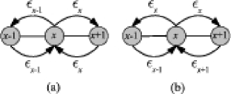
On the one hand, we have the random barrier (RB) model haus_diffusion_1987 ; bouchaud_anomalous_1990 . Physically this corresponds to the existence of a random potential barrier between every two neighboring sites so that the diffusion coefficient from site $x$ to site $x+1$ is equal to that from site $x+1$ to site $x$ (see Fig. 1). In other words, the disorder is associated with the bonds connecting neighboring sites on the lattice. We call this configuration model B:

$$\begin{array}[]{ll}\text{Model B:}&\left\{\begin{array}[]{lll}c_{x}&=&2\\ \sigma_{x,x-1}&=&\epsilon_{x}\\ \sigma_{x,x+1}&=&\epsilon_{x+1}\\ \sigma_{x,x}&=&(\epsilon_{x}+\epsilon_{x+1})/2\end{array},\right.\end{array}$$ (3)

where the disorder is drawn from a uniform distribution, $\epsilon_{x}\in\mathrm{U}(0,\epsilon_{0})$, and $\epsilon_{0}$ being an arbitrary parameter that we take as $1/3$ unless otherwise stated.

On the other hand, some disordered systems are better described by the so-called random trap (RT) model haus_diffusion_1987 ; bouchaud_anomalous_1990 . In this case a static disordered diffusion coefficient is assigned to each lattice site $x$ instead to bonds. This corresponds to our model C, which is defined by

$$\begin{array}[]{ll}\text{Model C:}&\left\{\begin{array}[]{lll}c_{x}&=&2\\ \sigma_{x,x-1}&=&\epsilon_{x-1}\\ \sigma_{x,x+1}&=&\epsilon_{x+1}\\ \sigma_{x,x}&=&\epsilon_{x}\end{array},\right.\end{array}$$ (4)

where the disorder is uniformly distributed, $\epsilon_{x}\in\mathrm{U}(0,\epsilon_{0})$, and again $\epsilon_{0}$ can be any number in the interval $(0,1/2)$, here we use $\epsilon_{0}=1/3$.

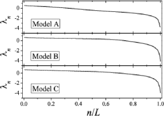
Typical Lyapunov spectra corresponding to the three disordered models introduced here are shown in Fig. 2 for a system of size $L=256$ and averages over 10 different disorder realizations. One can see that, depending on the model, one has 30-80 % of the spectra in the region $\lambda>0$. Note that Lyapunov spectra are self-averaging, therefore spectra for a single realization differ from the average in small fluctuations, which for large enough systems are negligible.

Some remarks are now in order. First, let us stress that these two disordered diffusion configurations, namely RB and RT, were not chosen arbitrarily, but are in fact all existing physically meaningful ways to introduce disorder in the diffusive couplings haus_diffusion_1987 ; bouchaud_anomalous_1990 . Second, it is important to remark that in this paper we focus on systems in the presence of weak disorder, where the probability density of having zero disorder at any given site, ${\cal P}(\epsilon=0)$, is bounded. We do leave out of our study the case of strong disorder, ${\cal P}(\epsilon\to 0)\sim\epsilon^{-|\nu|}$, where a fraction of the system sites can effectively act as sinks, which is known to have a great impact on the asymptotic transport properties haus_diffusion_1987 ; bouchaud_anomalous_1990 and will be discussed elsewhere.

Figure 2: Lyapunov spectra for models A, B and C in a lattice of $L=256$ coupled tent maps after average over ten different disorder realizations.

In principle, classical results on the problem of diffusion in random media haus_diffusion_1987 ; bouchaud_anomalous_1990 may also be invoked to argue that the details of the disorder distribution should be irrelevant in the sense that weak disorder gives rise to the same asymptotic dynamical behavior independently of the detailed form of the disorder distribution. The same conclusion applies in the case of strong disorder, where the asymptotic dynamics is fully determined by the form of the divergence at the origin, i.e. the value of the exponent $\nu$. In the following we focus on the case of weak disorder and a uniform distribution ${\cal P}(\epsilon)=\mathrm{U}(0,\epsilon_{0})$ with the parameter $\epsilon_{0}=1/3$ is used to exemplify our results. However, in the presence of random multiplicative terms the critical behavior might be affected by the detailed form of the disorder distribution krug1993 .

III Surface evolution and coarsening

As occurs in the case of homogeneous systems, the dynamics of the main LV can be conveniently described in terms of the equivalent surface picture pikovsky_roughening_1994 ; pikovsky_dynamic_1998 ; pikovsky_dynamic_2001 ; sanchez_rare_2004 ; szendro_CLV07 . The reason is that the logarithm of the perturbation field turns out to be scale-invariant, so that correlations have the form of power-law functions and critical exponents can then be used to characterize the space-time structure of perturbations. Therefore, in this paper we are interested in the scaling properties of the rough surface defined by the Hopf-Cole transform of the perturbation $h(x,t)\equiv\ln{|\delta u_{x}(t)|}=\ln{|\delta u_{x}(0)|}+\sum_{\tau=1}^{t}\ln{|\vartheta_{x}(\tau)|}$.

Space-time scaling properties of chaotic perturbations in inhomogeneous systems turn out to be very different from those in homogeneous systems, even in the case of weak disorder studied here. As can be immediately seen in Fig. 3, a first observation is the patterned structure of the LV surface, which is visible to the naked eye and contrasts with the KPZ-type morphologies observed in homogeneous systems pikovsky_roughening_1994 ; szendro_CLV07 . This already indicates that significant differences are to be expected in the scaling properties of inhomogeneous systems. Even weak disorder induces self-organization in a triangular structure, which reflects the strong spatial localization of the perturbation in the form of a exponential profile around some strong pinning centers. Note that a facet, $h(x,t)=h(x_{0})-s(t)|x-x_{0}|$, with a cusp at $x=x_{0}$ and slope $s(t)$ corresponds to an exponential profile of the perturbation, $\delta u_{x}(t)\propto\exp[-s(t)|x-x_{0}|]$, around the pinning center $x_{0}$.

Figure 3: Typical evolution a Lypunov vector surface $h(x,t)$. One can observe the emergence of facets that grow in time until, in the long time limit, the whole interface is spanned by one single facet. Tiny fluctuations can be observed at small scales. The data correspond to model C in a lattice of $L=1024$ maps.

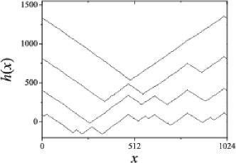
In Fig. 3 we plot a typical evolution of the main LV according to Eq. (II) in a system of size $L=1024$ for a given disorder realization in the case of model C. We observe that at short times, the surface $h(x,t)$ is composed of triangular facets of varying sizes which grow in time until, in the long time limit, the whole interface is formed by just one single facet. Therefore, as time evolves the size of the triangles increases and number of triangles diminishes. This surface dynamics corresponds to non-equilibrium ’coarsening’. Similar triangular morphologies are obtained for the three models A, B and C introduced above. Close inspection and analysis of critical exponents shows that the three models actually belong to different universality classes.

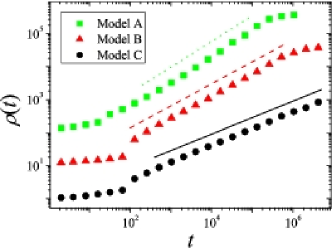
In order to characterize the growth of the faceted pattern we have measured the lateral mound size $\rho(t)$, which gives the coarsening length or typical length scale of the instability. This is usually done by calculating the slope-slope correlation function $\langle\overline{\nabla h(x,t)\nabla h(x+r,t)}\rangle$ and measuring the distance, $\rho(t)$, at which this correlation crosses zero. We calculate the surface gradient as the centered discrete derivative $\nabla h(x,t)\equiv[h(x+1,t)-h(x-1,t)]/2$. In Fig. 4 the lateral mound size, $\rho(t)$, for the three models is shown. After a short initial period, $\rho(t)$ grows as a power law in time with exponents $\theta_{\mathrm{B}}=0.67\pm 0.03$ and $\theta_{\mathrm{C}}=0.48\pm 0.03$, for models B and C, respectively. At long times $\rho(t)$ saturates, as the surface becomes dominated by a single facet and the coarsening length becomes comparable to the system size. For model A the intermediate region does not seems to be following a simple power-law. Nonetheless, we have fitted an exponent $\theta_{\mathrm{A}}=0.78\pm 0.05$ for the sake of comparison. The different scaling exponents for the coarsening length already indicate that the three models possibly belong to different universality classes.

Figure 4: (Color online) The evolution of the lateral mound size $\rho(t)$ is plotted for the three models. The straight lines are plotted to guide the eye and have slopes $0.78$ (dotted), $2/3$ (dashed) and $1/2$ (solid), respectively. The curves for models A and B have been shifted for better visibility.

IV Surface roughness scaling

Faceted surfaces exhibit anomalous scaling properties in the sense that local and global fluctuations may scale with different scaling functions (and exponents), which can be cast in the generic dynamic scaling form introduced by Ramasco et. al. ramasco_generic_2000 . In this section we briefly describe the generic scaling theory for surface kinetic roughening that will be used later on to analyze our numerical data.

The roughness of scale-invariant surfaces corresponds to the fluctuations of the surface height. These fluctuations can be computed either locally or globally as follows. On the one hand, the global roughness exponent $\alpha$ can be obtained from the scaling behavior of the global width $W(L,t)=\langle\overline{[h(x,t)-\overline{h}(t)]^{2}}\rangle^{1/2}$. Here, the overline denotes an average over all sites $x$ in a system of size $L$ and brackets denote the average over different realizations. For scale-invariant surfaces one expects the global width to scale as $W(L,t)=t^{\alpha/z}\mathcal{G}(L/t^{1/z})$, where $\mathcal{G}(u)$ is a scaling function that becomes constant for $u\gg 1$ and decays as $\sim u^{\alpha}$ for $u\ll 1$. The roughness exponent $\alpha$ and dynamic exponent $z$ characterize the scaling behavior of the global surface fluctuations.

On the other hand, one can measure the local roughness exponent $\alpha_{\mathrm{loc}}$, which is defined via the scaling behavior of the local width $w(l,t)=\langle\langle[h(x,t)-\langle h\rangle_{l}(t)]^{2}\rangle_{l}\rangle^{1/2}$, where $\langle\ldots\rangle_{l}$ denotes an average over $x$ in a window of size $l$. The local width scales as $w(l,t)\sim t^{\alpha/z}\mathcal{G}_{\mathrm{A}}(l/t^{1/z})$, where the scaling function $\mathcal{G}_{\mathrm{A}}(u)$ has a similar asymptotic behavior as $\mathcal{G}(u)$, but with a local anomalous exponent, $\sim u^{\alpha_{\mathrm{loc}}}$ for $u\ll 1$. So that in the stationary regime (for $t\gg L^{z}$) one obtains $w_{\mathrm{stat}}(l,L)\sim l^{\alpha_{\mathrm{loc}}}L^{\alpha-\alpha_{\mathrm{loc}}}$. In the cases where local and global roughness exponents do not coincide the scaling is said to be anomalous.

Figure 5: (Color online) The spectral power functions of the surfaces obtained for model A are plotted for times $t=2^{12}(\mathrm{a}),2^{14}(\mathrm{b}),2^{16}(\mathrm{c}),2^{18}(\mathrm{d})$. The straight line corresponds to $\alpha_{s}=1.5$. In the inset we show the data collapse according to the scaling ansatz (6) and (7), using $\alpha=1.03$ and $z=1.3$. The dashed and the solid straight line have slopes -1 and 3, respectively. The plotted data correspond to model A for a system of size $L=16384$ averaged over 100 disorder realizations.

Following Ramasco et. al. ramasco_generic_2000 , in order to correctly classify the different forms that scaling can take it is convenient to introduce a third roughness exponent, namely the so called spectral roughness exponent $\alpha_{\mathrm{s}}$. This is defined in terms of the structure factor (or power spectrum in $k$ space),

$$S(k,t)=\langle\widehat{h}(k,t)\widehat{h}(-k,t)\rangle,$$ (5)

where $\widehat{h}(k,t)$ is the spatial Fourier transform of $h(x,t)-\overline{h}(t)$. Ramasco et. al. ramasco_generic_2000 showed that scale-invariant roughening in $d+1$ dimensions is fully described in the following scaling ansatz:

$$S(k,t)=k^{-(2\alpha+d)}s(kt^{1/z}),$$ (6)

$z$ being the dynamical exponent that connects temporal-scales $\tau$ and length-scales $l$ according to $\tau\sim l^{z}$, and the nontrivial scaling function takes the form

$$s(u)\sim\left\{\begin{array}[]{lll}u^{2(\alpha-\alpha_{\mathrm{s}})}&\text{if}&u\gg 1\\ u^{2\alpha+d}&\text{if}&u\ll 1.\end{array}\right.$$ (7)

Here $\alpha$ is the global roughness exponent. With the help of these three exponents one can distinguish the four different possible types of scaling that any scale-invariant rough surface can exhibit,

$$\left\{\begin{array}[]{llll}\mathrm{if}&\alpha_{\mathrm{s}}<1\Rightarrow\alpha_{\mathrm{loc}}=\alpha_{\mathrm{s}}&\bigg{\{}\begin{array}[]{ll}\alpha_{\mathrm{s}}=\alpha\Rightarrow&\text{Family-Vicsek}\\ \alpha_{\mathrm{s}}\neq\alpha\Rightarrow&\text{intrinsic}\end{array}\\ \mathrm{if}&\alpha_{\mathrm{s}}>1\Rightarrow\alpha_{\mathrm{loc}}=1&\bigg{\{}\begin{array}[]{ll}\alpha_{\mathrm{s}}=\alpha\Rightarrow&\text{super-rough}\\ \alpha_{\mathrm{s}}\neq\alpha\Rightarrow&\text{faceted.}\end{array}\end{array}\right.$$ (8)

Note that only in the case where standard Family-Vicsek scaling is valid, which means $\alpha=\alpha_{\mathrm{loc}}=\alpha_{\mathrm{s}}$, the surface is self-affine. In the other cases this will in general not be true, i. e. local and global fluctuations will still exhibit dynamical scaling, but will do so with different exponents.

Although Family-Vicsek scaling is the best known scaling class barabasi_fractal_1995 , over the last ten years experimental studies in a variety of systems including growth of thin-films, electrodeposition, fracture or fluid imbibition yang_instability_1994 ; jeffries_instability_1996 ; huo_anomalous_2001 ; santamaria_scaling_2002 ; lopez_anomalous_1998 ; morel_anomalous_1998 ; soriano_anomalous_2002 as well as theoretical studies ramasco_generic_2000 ; amar_groove_1993 ; schroeder_scaling_1993 ; das_sarma_kinetic_1994 ; das_sarma_scale_1996 ; smilauer_crossover_1994 ; bhattacharjee_infrared_1996 ; dasgupta_controlled_1996 ; lopez_power_1997 ; lopez_superroughening_1997 ; krug_turbulent_1994 ; lopez_scaling_1999 ; lopez_scaling_2005 have confirmed the existence of intrinsic anomalous and super-rough kinetic roughening, as well as the validity of the generic scaling theory.

Figure 6: (Color online) The spectral power functions of interfaces obtained for model B are plotted for times $t=2^{12}(\mathrm{a}),2^{14}(\mathrm{b}),2^{16}(\mathrm{c}),2^{18}(\mathrm{d}),2^{20}(\mathrm{e})$. The straight line corresponds to $\alpha_{s}=1.5$. In the inset we show the data collapse according to scaling ansatz (6) and (7), using $\alpha=1.0$ and $z=1.5$. The dashed and the solid straight line have slopes -1 and 3, respectively. The plotted data corresponds to model B for a system of size $L=16384$ averaged over 100 realizations.

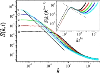
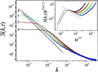
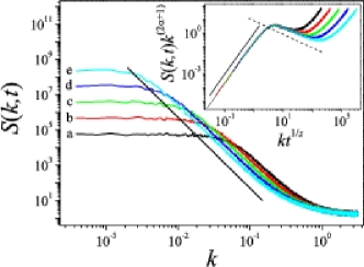
We now use this general scaling ansatz to study the scaling properties of our system. In order to do so, we have calculated the structure factor corresponding to the Hopf-Cole transforms of the perturbations at various times. Figures 5, 6 and 7 show the structure factor for models A, B and C, respectively. We observe a power-law decay as $\sim k^{-(2\alpha_{\mathrm{s}}+1)}$ for momenta limited by a large scale and a small scale cutoff. At large length scales the power-law behavior is limited by the correlation length $\xi(t)\sim t^{1/z}$, as expected from dynamical scaling. The cutoff at short lengths also grows in time, suggesting the existence of a different dynamics at small scales, which will be studied in detail in Sec. V. Note that the curves $S(k,t)$ shift downward for increasing times, indicating the presence of anomalous scaling with $\alpha_{\mathrm{s}}>\alpha$. Specifically, one expects $S(k,t)\sim k^{2\alpha_{\mathrm{s}}+1}t^{(\alpha-\alpha_{\mathrm{loc}})/z}$. We have measured $\alpha_{\mathrm{s}}=1.43\pm 0.05$, $1.47\pm 0.05$ and $1.45\pm 0.05$ for models A, B and C, respectively. This should be compared with the value of $\alpha_{\mathrm{s}}=3/2$ that can be obtained analytically for interfaces consisting of random smooth facets ramasco_generic_2000 . In the insets of Figs. 5, 6 and 7 we show a data collapse according to the generic scaling ansatz in Eqs. (6) and (7), obtaining values for the roughness and dynamical exponents $\alpha$ and $z$. As can be verified, all three models show scaling properties well described by the faceted interface scaling class in Ramasco’s classification, Eq. (8), with a roughness exponent $\alpha\approx 1$ for all the three models. Nonetheless, all three systems yield different values for the dynamical exponent, $z_{\mathrm{A}}=1.3\pm 0.1$, $z_{\mathrm{B}}=1.50\pm 0.03$ and $z_{\mathrm{C}}=2.00\pm 0.03$, again indicating that the three models belong to different universality classes. These values of $z$ define the typical length scale that correlations have spread along the system up to time $t$, $\xi(t)\sim t^{1/z}$, and are in good agreement with the inverse of the exponents ($\theta=1/z$) that we obtained from the analysis of the coarsening length discussed in Sec. III for all the three models studied in this paper.

Figure 7: (Color online) The spectral power functions of interfaces obtained for model C are plotted for times $t=2^{12}(\mathrm{a}),2^{14}(\mathrm{b}),2^{16}(\mathrm{c}),2^{18}(\mathrm{d}),2^{20}(\mathrm{e})$. The straight line corresponds to $\alpha_{s}=1.5$. In the inset we show the data collapse according to scaling ansatz (6) and (7), using $\alpha=1.0$ and $z=2.0$. The dashed and the solid straight line have slopes -1 and 3, respectively. The plotted data corresponds to model C for a system of size $L=16384$ averaged over 100 realizations.

V Separating facets from fluctuations

The scaling analysis of the surface fluctuations presented in the preceding sections has shown that the LV surface self-organizes in a characteristic triangular pattern for all the three models of disorder. A closer inspection, in particular the computation of the structure factor, has also revealed the existence of a cutoff at small scales such that length scales below that point obey a different dynamics. This suggests the existence of another dynamical process taking place at small scales which is different from the mechanism responsible for the large scale faceted structure.

Figure 8: For a segment of 1024 maps on a system of $L=16364$ we exemplify the separation of the surface $h(x)$ into the triangular pattern $h^{0}(x)$ and the difference $y(x)=h(x)-h^{0}(x)$, which gives the small scale fluctuations.

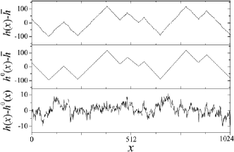
In this section we show that one can actually separate two different contributions to the LV surface height: The large scale pattern, $h^{0}(x,t)$, formed by facets of constant slope, and a randomly fluctuating term, $y(x,t)$, which becomes the dominant one at small scales. Therefore the surface profile at any given time can be expressed as the sum of the two independent components as $h(x,t)=h^{0}(x,t)+y(x,t)$. This separation can be carried out numerically as follows. For a given time the interface $h(x,t)$ is smoothed to remove local maxima and minima corresponding to local fluctuations upon the triangular structure. This is done by replacing the heights at every site by a spatial average over some arbitrary region around each site. Then, the locations of the cusp sites and valley sites of the smoothed curve are easily identified and the faceted pattern $h^{0}(x)$ is defined as the set of straight lines connecting the cusp points to the neighboring valley points. The interface corresponding to the fluctuations is then obtained by taking the difference $y(x,t)=h(x,t)-h^{0}(x,t)$ as exemplified in Fig. 8

Interestingly, one can observe that the triangular pattern, $h^{0}$, and the random fluctuation components, $y(x,t)$, are uncorrelated. This can be shown by checking that $\langle\widehat{h^{0}}(k,t)\widehat{y}(-k,t)\rangle=0$, which is equivalent to proving the identity

$$S(k,t)=\langle\widehat{h^{0}}(k,t)\widehat{h^{0}}(-k,t)\rangle+\langle\widehat{y}(k,t)\widehat{y}(-k,t)\rangle.$$ (9)

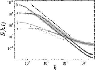
In fact, the numerical data presented in Fig. 9 confirm that both components are actually uncorrelated. Figure 9 shows the structure factor of the faceted pattern $h^{0}(x,t)$, the local fluctuations $y(x,t)$, and the complete interface $h(x,t)$ at two different times. In particular, the data shown correspond to model B, but we obtained identical results for for the other two models.

It becomes apparent that the anomalous scaling of the surface stems from that of the faceted structure. Since the vertical scale in Fig. 9 is logarithmic, the sum in Eq. (9) will essentially be dominated by the largest of the two terms, as one can easily see in Fig. 9. Therefore, the large scale behavior of the complete interface is totally dominated by the scaling behavior of the pattern component. On the other hand, the structure factor $S(k,t)$ should crossover to that of the local fluctuations, $\langle\widehat{y}(k,t)\widehat{y}(-k,t)\rangle$, at short wavelengths. The structure factor of the pattern component shifts downwards with time because $\alpha<\alpha_{\mathrm{s}}$. This is not the case for the structure factor of the local fluctuations, which scale according to Family-Vicsek’s, where $\alpha=\alpha_{\mathrm{s}}\approx 0.45$ is fulfilled. Thus the length scale at which the local fluctuations dominate the structure factor should grow with time. Whether the asymptotic scaling behavior of the facets can be observed in the limit $t\rightarrow\infty$ for a finite system depends on the relative strength of the local fluctuations.

Figure 9: The power spectra of the interface $h(x)$ (light gray dots), the triangular structure $h^{0}(x)$ (dark gray lines), and the difference $y(x)=h(x)-h^{0}(x)$ (gray lines) are plotted for two different times $t_{\mathrm{a}}<t_{\mathrm{b}}$. The straight solid line corresponds to $\alpha^{0}_{\mathrm{s}}=1.5$, while the straight dashed line corresponds to $\alpha^{\mathrm{diff}}_{\mathrm{s}}=0.45$.

VI Lyapunov vectors

So far we have studied the dynamics of random infinitesimal perturbations, which is equivalent to study the dynamics of the most unstable direction in tangent space, i. e. the first LV. We now devote this section to briefly describe the dynamics of further unstable directions that growth at slower rates.

Let us start by introducing a few key quantities that shall be used in our analysis. The evolution equation for an initially random infinitesimal perturbation, Eq. (II), can be written in vectorial form as $\mathbf{\delta u}(t+1)=\mathbf{J}[\mathbf{u}(t)]\mathbf{\delta u}(t)$, where $\mathbf{J}[\mathbf{u}(t)]$ is just the jacobian evaluated on the trajectory $\mathbf{u}(t)$ at time $t$. Since infinitesimal perturbations evolve linearly there exists a linear operator $\mathbf{M}(t_{2},t_{1})$ such that $\mathbf{\delta u}(t_{2})=\mathbf{M}(t_{2},t_{1})\mathbf{\delta u}(t_{1})$, given by $\mathbf{M}(t_{2},t_{1})=\prod_{t_{i}=t_{1}}^{t_{2}-1}\mathbf{J}[\mathbf{u}(t_{i})]$. Oseledec’s theorem Oseledec1968 implies that the (symmetric) limit operator $\lim_{t_{2}\rightarrow\infty}[\mathbf{M}(t_{2},t_{1})\mathbf{M}^{*}(t_{2},t_{1})]^{1/2(t_{2}-t_{1})}$, where $\mathbf{M}^{*}$ denotes the adjoint of $\mathbf{M}$, does exist and the logarithms of its eigenvalues are the Lyapunov exponents $\lambda_{n}$ ($n=1,2,\cdots,L$) and the eigenvectors are the so-called backward Lyapunov vectors $\mathbf{b}_{n}$ eckmann ; legras96 . In what follows, we will consider standard ordering of the Lyapunov exponents, $\lambda_{1}\geq\lambda_{2}\geq\ldots\geq\ldots\lambda_{L}$, and the corresponding vectors. We use standard numerical techniques to calculate Lyapunov exponents and vectors benettin_lyapunov_1980 ; GEIST1990 .

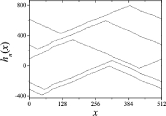
As we have discussed in Secs. III and IV, in inhomogeneous systems the main LV, the one corresponding to the most unstable direction, converges to a faceted structure asymptotically dominated by one single facet in the limit $t\rightarrow\infty$. In Fig. 10 we plot the LV surfaces $h_{n}(x,t)=\ln(|b_{n}(x,t)|)$, $n\in\{1,2,3,4,5\}$, corresponding to the first five backward LVs for model B at some arbitrary time $t$ during evolution in a system of 512 coupled maps. The surface profiles in this plot are arbitrarily shifted in the vertical direction to aid comparison. In the long time limit the interface $h_{1}(x,t)$, the first LV surface, naturally coincides with the interface $h(x,t)$ corresponding to an arbitrary initially random perturbation. It should be observed that not only the first LV, but each surface $h_{n}(x,t)$ corresponding to the $n$-th LV indeed converges to a structure dominated by a single triangle as well. This is actually the case for all the inhomogeneous models studied in this paper.

Interestingly, the location of the cusp of the triangles, where the LVs spatially localize, is not arbitrary. It is interesting to compare the positions of the global maxima of the interface profiles with the values of the quenched disorder at those sites. For model C, i. e. the RT case, the site where the first LV takes its maximum value coincides with the site $x$ at which the coupling $\epsilon_{x}$ takes its lowest value, the site where the second LV takes its maximum coincides with the site where $\epsilon_{x}$ takes its second lowest value, and so forth. This is easy to interpret: since errors get trapped at sites with lower diffusion, the result is that the LVs strongly localize and utterly get frozen at those sites.

A very similar correlation effect between error localization and disorder can be seen for model B, i. e. the RB case. Note that in the case of RB disorder the diffusion coefficient at a given site $x$ is the sum $\epsilon_{x+1}+\epsilon_{x}$ of the local diffusive couplings connecting $x$ to any of the two neighboring sites. In fact, we find that the site where the first LV takes its maximum coincides with the site $x$ where the diffusivity $\epsilon_{x+1}+\epsilon_{x}$ takes its lowest value, the site where the second LV takes its maximum value coincides with the site where $\epsilon_{x+1}+\epsilon_{x}$ takes its second lowest value and so forth. Thus, the on-site growth velocity is again controlled by the probability for the perturbation to get trapped at that site.

One would expect that a similar association of LVs maxima with disorder extrema should also exist for model A. However, things are not that straightforward in this case. We recall that in model A the disorder is introduced in the map constants and not in the diffusive couplings, which are identical along the system. We think that due to the dominance of small scale fluctuations up to quite large length scales for model A (see Fig. 5) as compared with the situation for models B and C, the maxima get smoothed out and an extended neighborhood, rather than just one single site, controls the final position where the LVs get frozen at long times. In other words, local synchronization of neighboring sites over short scales makes it difficult to simply identify the region where, at a coarse-grained level, the vectors will get asymptotically trapped in the case of disorder of type A.

Figure 10: The surfaces $h_{n}(x)$ corresponding to the first five Lyapunov-vectors are plotted (from bottom $n=1$ to top $n=5$). Note that all the interfaces converge to a triangular structure. The data presented were obtained for model B and have been shifted for better visibility.

VII Torward a phenomenological stochastic field theory

The evolution of perturbations in homogeneous SECSs is known to be described in statistical terms by the multiplicative stochastic equation

$$\frac{\partial}{\partial t}\delta u=\partial_{xx}\delta u+\xi(x,t)\delta u,$$ (10)

where $\xi(x,t)$ is a noise term that accounts for the chaotic fluctuations along the trajectory and is assumed to be delta-correlated in space and time, $\langle\xi(x,t)\,\xi(x^{\prime},t^{\prime})\rangle=2\,\sigma\,\delta(x-x^{\prime})\,\delta(t-t^{\prime})$. Pikovsky and Kurths pikovsky_roughening_1994 and Pikovsky and Politi pikovsky_dynamic_1998 proposed this equation as the proper candidate for modeling the dynamics of the first Lyapunov vector from a statistical perspective. They showed that it actually reproduces the main statistical properties of SECS in a variety of systems pikovsky_dynamic_1998 . This equation mimics the linear equations in tangent space for the dynamics of infinitesimal perturbations in spatio-temporal chaotic systems.

An important feature of Eq. (10) is that, under a Hopf-Cole transformation, $h=\ln|\delta u|$, it maps into the KPZ equation:

$$\frac{\partial}{\partial t}h=(\partial_{x}h)^{2}+\partial_{xx}h+\xi(x,t),$$ (11)

which ultimately justifies why the log-transformed (main) Lyapunov vector of many spatiotemporal chaotic systems scales in space and time as a KPZ surface pikovsky_roughening_1994 ; pikovsky_dynamic_1998 ; pikovsky_dynamic_2001 ; sanchez_rare_2004 ; szendro_CLV07 . Interestingly, Eq. (10) also appears in the context of the classical problem of the directed polymer in a random potential kardar_zhang (also see Ref. halpin-zhang for an detailed review).

We now explore extensions of this type of Langevin equations to the case of disordered systems. A phenomenological stochastic field theory of this kind should be helpful in order to identify the essential symmetries and mechanisms that determine the dynamics of perturbations in chaotic disordered systems. The existence of scale invariance strongly encourages this approach. Therefore, microscopic details of the models are expected to be irrelevant at a sufficiently coarse-grained scale, as occurs in the case of homogeneous systems.

In the case of Model A, Eq. (II) can be considered as a straightforward discrete version of

$$\frac{\partial}{\partial t}\delta u=\partial_{xx}[\partial_{u}f(x,u)\delta u]+[\partial_{u}f(x,u)-1]\,\delta u.$$

It is important to note that the noisy term $\partial_{u}f(x,u)\equiv\partial_{y}f(x,y)|_{u(x,t)}$ depends implicitly on time through the trajectory $u(x,t)$ and so, it includes both an annealed and a quenched component. The origin of the latter is the inhomogeneous character of the coupled elements: Sites are more or less chaotic depending on their position $x$ in the system. For instance, in the particular case of the logistic map we have $\partial_{u}f(x,u)=c(x)[1-2c(x)u]$, where $c(x)$ is the local map parameter. We argue that in the hydrodynamic limit the quenched part of the noise dominates over the annealed one. The reason being that the quenched character of the disorder generates long-range temporal correlations at each site, which are expected to control the dynamics over the short-range correlations of the annealed random terms.

These arguments suggest that for type A models the long time limit of main LV should be generically described by a multiplicative Langevin equation like

$$\frac{\partial}{\partial t}\delta u=\partial_{xx}[(\zeta(x)\delta u]+\partial_{xx}\delta u+\zeta(x)\delta u,$$ (12)

where $\zeta(x)$ represents the quenched disorder. This equation can be further simplified since the disordered diffusion term $\partial_{xx}[(\zeta(x)\delta u]$ is irrelevant as compared with $\partial_{xx}\delta u$. To be precise, in the case of weak disorder that we study here the inhomogeneous diffusion term simply renormalizes to an effective constant diffusion term . Finally we arrive at our stochastic field theory proposal for model A type of systems:

$$\partial_{t}\delta u=D\partial_{xx}\delta u+\zeta(x)\delta u,$$ (13)

where $D$ is an effective diffusion constant and $\zeta(x)$ is a quenched columnar disorder with delta correlations.

Interestingly, Eq. (13) appears in the context of diffusion in random trapping/amplifying quenched potentials zhang_diffusion_1986 ; ebeling_diffusion_1984 ; engel_comment_1987 ; tao_exact_1988 ; tao_exact_1989 ; tao_path-integral_1991 ; rosenbluth_random_1989 ; valle_diffusion_1991 . After the Hopf-Cole transform of the perturbation field, $\delta u=\exp(\mu h/D)$, one obtains

$$\partial_{t}h(x,t)=\partial_{xx}h+\mu(\partial_{x}h)^{2}+\zeta(x),$$ (14)

which is a close relative of the KPZ equation, but here the additive noise term $\zeta(x)$ is quenched and delta correlated, $\langle\zeta(x)\zeta(x^{\prime})\rangle=2\theta\delta(x-x^{\prime})$. This equation has attracted some interest in the past, as it also describes the free energy of directed and undirected polymers of length $t$ in the presence of columnar disorder CATES1988 ; nattermann_diffusion_1989 ; krug1993 ; szendro_localization_2007 .

Only very recently szendro_localization_2007 , it has been realized that the surface described by Eq. (14) exhibits anomalous scaling exponents induced by the self-organization in a faceted structure. In Ref. szendro_localization_2007 we studied Eq. (14) by means of extensive simulations and determined the critical exponents to be $z=1.35\pm 0.05$, $\alpha=1.05\pm 0.05$ and $\alpha_{\mathrm{s}}=1.50\pm 0.05$. These values are in excellent agreement with the values reported here for the critical exponents of the main LV surface in SECSs of type A (see Fig. 5). This strongly supports our claim that, in fact, Eq. (13) is a minimal model that captures the essential ingredients dominating the evolution of errors in inhomogeneous models of type A .

As it has already been discussed in Ref. szendro_localization_2007 , the introduction of an additional annealed noise term in Eq. (14) is irrelevant in the renormalization group sense, but leads to an increase of the typical size over which the local random fluctuations (discussed in Sec. V) dominate. Hence, for a finite size system the asymptotic scaling behavior may not be observable if the thermal noise amplitude is too large. This is of some importance for the situations we are interested in because, when considering the evolution of perturbations in SECS, there will always be some temporally fluctuating noise as explained above. Thus, even if quenched disorder is present in the studied system, it may be very weak in comparison with the temporally fluctuating one. In that case the behavior described here would only be observable in very large systems.

Moreover, it should be noticed that, although the roughness exponents $\alpha$, $\alpha_{\mathrm{loc}}$ and $\alpha_{\mathrm{s}}$ seem to be the same within error bars for the three models of disorder studied in this paper, the dynamic exponent $z$ does take different values. This suggests that the disorder symmetries that distinguish models A, B and C are indeed relevant and lead to different nonequilibrium universality classes. One can try to formulate a stochastic-field evolution equation similar to Eq. (12) for models B and C, but where the disorder enters in a different form into the diffusion and the multiplicative term in order to reflect the different symmetries of the coupling in these two models. Unfortunately, we have not been able to find the correct equations reproducing the scaling behavior of the LV surfaces for disordered systems in the class B and C. Similar arguments might be used to write down the stochastic equation

$$\partial_{t}\delta u=\partial_{x}[\zeta(x)\partial_{x}\delta u]+\xi(x,t)\delta u,$$ (15)

for model B and

$$\partial_{t}\delta u=\partial_{xx}[\zeta(x)\delta u]+\xi(x,t)\delta u,$$ (16)

for model C, where $\xi(x,t)$ is a noise term. We have investigated the scaling properties of Eqs. (15) and (16) by means of numerical simulations and found that, while these simple stochastic models generically lead to faceted surfaces with the expected roughness exponents, they are unable to reproduce the correct dynamic exponent of disordered SECS in the class B nor C. We believe that the reason behind this disagreement lies in the existence of correlations between the quenched and annealed fluctuating terms that are not incorporated in this naive approach. These non-trivial correlations might also explain the, at least at first sight, counter intuitive result that different dynamic exponents are observed in SECS of class B and C. Some remarks regarding this point are now in order.

Classical diffusion in random media involves the study of equations like (15) and (16), but where the multiplicative term $\xi(x,t)\delta u$ is absent. It is well-known bouchaud_anomalous_1990 that, in the long time limit, dynamics of RB and RT models is identical, even for strong disorder. Despite the different symmetries involved, the large scale physics is the same. However, our numerical results indicate that model B (RB symmetry) and model C (RT symmetry) in SECS seemingly belong to different universality classes. We claim that the multiplicative noise, which is generically coupled to the quenched disorder in the systems we have studied, breaks the duality between RB and RT type of disorder in this case, leading to distinct dynamical exponents for the two different diffusion configurations.

VIII Conclusions

We have studied the evolution of infinitesimal perturbations in inhomogeneous spatially extended systems exhibiting space-time chaos. Inhomogeneity is introduced by means of a quenched disorder. We have considered one-dimensional coupled-map lattices as a simple and computationally convenient model system to analyze some aspects of chaos in the presence of disorder. In this regard, three different classes of models have been investigated by means of extensive numerical simulations. In all cases we find a strong localization behavior characterized by an exponential spatial profile around some localization centers. In the long time limit the perturbation concentrates around one single final attracting center. We have also studied the second, third, and so on backward LVs corresponding to most rapidly expanding directions in tangent space and found a correspondence between the localization centers and the positions in space corresponding to increasing minima of the diffusion in the particular disorder realization.

Note that the strong localization behavior described here is essentially different from the dynamic localization observed in the case of homogeneous SECS. In the latter, perturbations do also localize on just a few sites, but the position of these sites keeps fluctuating in time. However, in the presence of quenched disorder the sites where perturbations localize are fixed by the corresponding realization of the disorder.

Moreover, by a standard mapping (Hopf-Cole transform) of the perturbation into a growing surface we found that the LV associated surfaces self-organize in a faceted structure, at variance with what occurs in homogeneous (non disordered) systems where one generically obtains a surface in the universality class of KPZ. Interestingly, this faceted surface was found to exhibit coarsening and anomalous kinetic roughening in agreement with previous theoretical predictions ramasco_generic_2000 for this type of scale-invariant structures.

The evolution of infinitesimal perturbations in spatially extended chaotic systems with quenched disorder may be described at a coarse-grained level as a diffusion process in a random potential. Note, however, that the value of the dynamical exponent $z$ depends on how disorder is introduced. The reason for this is possibly the influence of the disorder distribution on the temporal dependence of the coarsening, as described in Ref. krug1993 in the context of diffusion (see also Ref. szendro_localization_2007 for a discussion relevant to the present work)

We think that strong localization and anomalous scaling should play a role, e. g. in realistic weather models, where quenched disorder is included in the form of inhomogeneous boundary conditions representing certain geographical and topographical conditions.