High order relaxed schemes for nonlinear reaction diffusion problems in nonconservative form

Abstract

Different relaxation approximations to partial differential equations, including conservation laws, Hamilton-Jacobi equations, convection-diffusion problems, gas dynamics problems, have been recently proposed. The present paper focuses onto diffusive relaxed schemes for the numerical approximation of nonlinear reaction diffusion equations. We choose here a nonstandard relaxation scheme that allow the treatment of diffusion equations in their nonconservative form. A comparison with the traditional approach in the case of conservative equations is also included. High order methods are obtained by coupling ENO and WENO schemes for space discretization with IMEX schemes for time integration, where the implicit part can be explicitly solved at a linear cost. To illustrate the high accuracy and good properties of the proposed numerical schemes, also in the degenerate case, we consider various examples in one and two dimensions: the Fisher-Kolmogoroff equation, the porous-Fisher equation and the porous medium equation with strong absorption. Moreover we show a test on a system of PDEs that describe an ecological model for the dispersal and settling of animal populations.

1 Introduction

The main purpose of this work is to approximate solutions of a nonlinear, possibly degenerate, reaction-diffusion equation of the form

$$\frac{\partial u}{\partial t}=D\nabla\cdot(A(u)\nabla u)+g(u)$$ (1)

for $x\in\Omega\subseteq\mathbb{R}^{d},~{}~{}d\geq 1,~{}~{}t\geq 0$, with initial condition, $u(x,0)=u_{0}(x)$ and with suitable boundary conditions, where the function $A$ is a non-negative bounded function defined on $\mathbb{R}$. The equation is degenerate if $A(0)=0$ and in this case the solutions often become non-smooth in finite time, developing fronts and discontinuities [Aro70]. Finally, the coefficient $D$ is a diffusivity coefficient and the function $g(u)$ is the reaction term.

Equations like (1) are relevant in describing biological and physical processes and are involved in the modelling of population growth and dispersal [GRSGM00, TLB07a], of waves of concentration of chemical substances in living organisms, of the motion of viscous fluids (see e.g. [Mur02]). Also, systems of equations like (1), coupled via the reaction terms, are capable of modelling the cyclic Belousov-Zhabotinskii reactions and the pattern formation on the wings of butterflies and the coat of mammals (see [Mur03] and references therein).

This paper is organized as follows. In section 2 we introduce the relaxation approximation of nonlinear diffusion problems, in section 3 we describe the fully discrete relaxed numerical scheme in the reaction-diffusion case. In section 4 we report several numerical tests, in one and two space dimensions. The last application shown is about a relevant ecological model.

2 Relaxation approximation of nonlinear diffusion

The schemes proposed in the present work are a generalization of those proposed and studied in [NP98], and fit in the wider class of the schemes associated to relaxation approximations of partial differential equations, started after the well-known case studied in [JX95] for hyperbolic conservation laws. In the case of the nonlinear diffusion operator in (1), an additional variable $\vec{v}(x,t)\in\mathbb{R}^{d}$ and a positive parameter $\varepsilon$ are introduced and the following relaxation system is considered:

$$\left\{\begin{array}[]{ll}\displaystyle\frac{\partial u}{\partial t}+\mathrm{div}(\vec{v})=g(u)\\ \\ \displaystyle\frac{\partial\vec{v}}{\partial t}+\frac{D}{\varepsilon}A(u)\nabla u=-\frac{1}{\varepsilon}\vec{v}\end{array}\right.$$ (2)

Now, formally, in the small relaxation limit, $\varepsilon\rightarrow 0^{+}$, system (2) approximates to leading order equation (1).

We point out that in this relaxation system we do not need a third equation to “relax” the non-linearity of $A$, as was the case in [CNPS07].

In the previous system the parameter $\varepsilon$ has physical dimensions of time and represents the so-called relaxation time. Furthermore, each component of $\vec{v}$ has the dimension of $u$ times a velocity and $\varphi$ is a velocity. The inverse of $\varepsilon$ gives the rate at which $v$ decays onto $-A(u)\nabla u$ in the evolution of the variable $\vec{v}$ governed by the stiff second equation of (2).

In order to justify the convergence of the proposed relaxation scheme to equation (1), we study the Chapman-Enskog expansion of the solutions of (2). We consider for simplicity the case with only one spatial variable and temporarily assume that $A$ is sufficiently regular. From the second equation of (2) we obtain

$$v=-A(u)u_{x}-\varepsilon v_{t}=-A(u)u_{x}-\varepsilon(A(u)u_{x})_{t}+O(\varepsilon^{2})$$

Using the relation above and (2) again, one computes

$$\begin{split}(A(u)u_{x})_{t}=A^{\prime}(u)u_{t}u_{x}+A(u)u_{tx}=A^{\prime}(u)(-v_{x})u_{x}+A(u)(-v_{x})_{x}\\ =-(A(u)v_{x})_{x}=\left(A(u)\left(A(u)u_{x}\right)_{x}\right)_{x}+O(\varepsilon)\end{split}$$

Finally we substitute in the first equation of (2), obtaining

$$u_{t}-\left(A(u)u_{x}\right)_{x}=\varepsilon\left(A(u)\left(A(u)u_{x}\right)_{x}\right)_{xx}+O(\varepsilon^{2})$$

The idea of employing a semilinear hyperbolic relaxation system to derive numerical schemes for (degenerate) diffusion equation was first introduced in [NP00] for the purely diffusive case in the conservative form $u_{t}=\mathrm{\Delta}(p(u))$. High order schemes based on such approach have been studied in [CNPS07]. As in that paper we introduce a parameter $\varphi$ which allows to move the stiff terms $\frac{D}{\varepsilon}\nabla p(u)$ to the right hand side, without losing the hyperbolicity of the system:

$$\left\{\begin{array}[]{ll}\displaystyle\frac{\partial u}{\partial t}+\mathrm{div}(\vec{v})=g(u)\\ \\ \displaystyle\frac{\partial\vec{v}}{\partial t}+\varphi^{2}\nabla u=-\frac{1}{\varepsilon}\vec{v}+\left(\varphi^{2}\nabla u-\frac{D}{\varepsilon}A(u)\nabla u\right)\end{array}\right.$$ (3)

Now, the characteristic velocities of the hyperbolic left hand side are given by $\pm\varphi$ and are no longer stiff.

We point out that degenerate parabolic equations often model physical situations where free boundaries and discontinuities are relevant: we expect that schemes for hyperbolic systems will be able to reproduce faithfully these details of the solution. One of the main properties of (2) consists in the semilinearity of the system, that is all the nonlinear terms are in the (stiff) source terms, while the differential operator is linear. Hence, the solution of the convective part requires neither Riemann solvers nor the computation of the characteristic structure at each time step, since the eigenstructure of the system is constant in time. Moreover, the relaxation approximation does not exploit the form of the nonlinear function $A$ and hence it gives rise to a numerical scheme that, to a large extent, is independent of it, resulting in a very versatile tool.

We also anticipate here that, in the relaxed case (i.e. $\varepsilon=0$), the stiff source terms can be integrated solving a system that is already in triangular form and then it does not require iterative solvers.

Obviously, when (1) can be put in the form $u_{t}+\mathrm{\Delta}(p(u))=g(u)$, the relaxation approximation of the parabolic part described in [CNPS07] can be employed. In the following sections we will compare the two possibilities from a theoretical and numerical point of view.

3 Relaxed numerical schemes

The numerical approximation of system (3) can be obtained following the ideas already exploited in [CNPS07]: first obtain a semidiscrete scheme applying an IMEX time integrator and then choose a high order non-oscillatory spatial discretization. The reaction term will be included in the explicit part of the IMEX scheme. This obviously is convenient only for non-stiff reaction terms.

For simplicity, here we describe the one-dimensional case, the generalization being straightforward.

3.1 Relaxed IMEX schemes

We observe that system (3) is in the form

$$\frac{\partial{z}}{\partial{t}}+\frac{\partial{f(z)}}{\partial{x}}=g(z)+\frac{1}{\epsilon}h(z)$$

where $z=(u,v)^{T}$, $f(z)=(v,\varphi^{2}u)^{T}$, $g(z)=(g(u),0)^{T}$ and $h(z)=(0,-v+\varepsilon\varphi^{2}u_{x}-DA(u)u_{x})^{T}$. When $\varepsilon$ is small, the presence of both non-stiff and stiff terms, suggests the use of IMEX schemes [ARS97, KC03, PR05]. In the problems considered here, the reaction term $g(u)$ is not stiff and hence we treat it within the explicit portion of the IMEX scheme.

First we semi-discretize the equation in time. Let’s assume for simplicity a uniform time step $\Delta t$ and denote with $z^{n}$ the numerical approximation of the variable $z$ at time $t_{n}=n\Delta t$, for $n=0,1,\ldots$ We employ a $\nu$-stages IMEX scheme including the $1/\varepsilon$ terms in the implicit part, giving

$$z^{n+1}=z^{n}-\Delta t\sum_{i=1}^{\nu}\tilde{b}_{i}\left[\frac{\partial{f}}{\partial{x}}(z^{(i)})+g(z^{(i)})\right]+\frac{\Delta t}{\varepsilon}\sum_{i=1}^{\nu}b_{i}h(z^{(i)})$$ (4)

where the stage values are computed as

$$z^{(i)}=B^{(i)}+\frac{\Delta t}{\varepsilon}a_{i,i}h(z^{(i)})$$ (5)

for

$$B^{(i)}=z^{n}-\Delta t\sum_{k=1}^{i-1}\tilde{a}_{i,k}\left[\frac{\partial{f}}{\partial{x}}(z^{(k)})+g(z^{(k)})\right]+\frac{\Delta t}{\varepsilon}\sum_{k=1}^{i-1}a_{i,k}h(z^{(k)})$$ (6)

Here $({a}_{ik},{b}_{i})$ and $(\tilde{a}_{ik},\tilde{b}_{i})$ are a pair of Butcher’s tableaux [HNW93] of, respectively, a diagonally implicit and an explicit Runge-Kutta scheme.

In this work we use the so-called relaxed schemes, that are obtained by letting $\varepsilon\rightarrow 0$ in (4). The first stage, that is (5) with $i=1$, is defined by

$$\lim_{\varepsilon\to 0}\left\{\left[\begin{array}[]{l}{u^{(1)}}\\ {v^{(1)}}\\ \end{array}\right]-\left[\begin{array}[]{l}u^{n}\\ v^{n}\end{array}\right]-\frac{\Delta t}{\varepsilon}a_{1,1}h\left(\left[\begin{array}[]{l}u^{(1)}\\ v^{(1)}\end{array}\right]\right)\right\}=0$$ (7)

and thus

$${u^{(1)}=u^{n}}\qquad v^{(1)}=-A(u^{(1)})\frac{\partial{u^{(1)}}}{\partial{x}}.$$

Note that, in particular, $h(z^{(1)})=0$. Now the second stage, $i=2$, reads

$$z^{(2)}=z^{n}-\Delta{t}\tilde{a}_{2,1}{\left[\frac{\partial{f}}{\partial{x}}(z^{(1)})+g(z^{(1)})\right]}+\frac{\Delta t}{\varepsilon}a_{2,1}\underbrace{{h(z^{(1)})}}_{{\equiv 0}}+\frac{\Delta t}{\varepsilon}a_{2,2}{h(z^{(2)})}.$$

Hence the second component of $z^{(2)}$ is determined by the stiff term of the above expression, namely $h(z^{(2)})=0$. On the other hand, due the form of $h(z)$, there are no stiff terms in the equation for the first component $u^{(2)}$, which is then determined by a balance law.

Summarizing, the relaxed scheme yields an alternation of relaxation steps

$$h(z^{(i)})=0\qquad\text{ i.e. }\,v^{(i)}=-A(u^{(i)})\frac{\partial{u^{(i)}}}{\partial{x}}$$ (8)

and transport steps where we advance for time $\tilde{a}_{i,k}\Delta{t}$

$$\frac{\partial{z}}{\partial{t}}+\frac{\partial{f(z)}}{\partial{x}}=g(z)$$ (9)

with initial data $z=z^{(i)}$, retain only the first component and assign it to $u^{(i+1)}$. Finally the value of $u^{n+1}$ is computed as $u^{n}+\sum\tilde{b}_{i}u^{(i)}$.

3.2 Spatial reconstructions

In order to have a fully discrete scheme, we still need to specify the space discretization. We will use discretizations based on finite differences, in order to avoid cell coupling due to the source terms.

Recall that the IMEX technique reduces the integration to a cascade of relaxation and transport steps. The former are the implicit parts of (7) and (5), while the transport steps appear in the evaluation of the explicit terms $B^{(i)}$ in (6). Since (7) and (5) involve only local operations, the main task of the space discretization is the evaluation of $\partial_{x}{f}$, where we will exploit the linearity of $f$ in its arguments.

In the one-dimensional case, let us consider a uniform grid on $[a,b]\subset\mathbb{R}$, $x_{j}=a-\frac{h}{2}+jh$ for $j=1,\ldots,m$, where $h=(b-a)/m$ is the grid spacing and $m$ the number of cells. We denote with $z^{n}_{j}$ the value of the quantity $z$ at time $t^{n}$ at $x_{j}$, the centre of the $j^{\mbox{\scriptsize th}}$ computational cell. The fully discrete scheme may be written as

$$z_{j}^{n+1}=z_{j}^{n}-\Delta t\sum_{i=1}^{\nu}\tilde{b}_{i}\left(F^{(i)}_{j+1/2}-F^{(i)}_{j-1/2}\right)+\frac{\Delta t}{\varepsilon}\sum_{i=1}^{\nu}b_{i}g(z_{j}^{(i)}),$$

where $F^{(i)}_{j+1/2}$ are the numerical fluxes, which are the only item that we still need to specify. It is necessary to write the scheme in conservation form and thus, following [SO89], we introduce the function $\hat{F}$ such that

$$f(z(x,t))=\frac{1}{h}\int_{x-h/2}^{x+h/2}\hat{F}(s,t)\mathrm{d}s$$

and hence

$$\frac{\partial f}{\partial x}(z(x_{j},t))=\frac{1}{h}\left(\hat{F}(x_{j+1/2},t)-\hat{F}(x_{j-1/2},t)\right).$$

The numerical flux function $F_{j+1/2}$ approximates $\hat{F}(x_{j+1/2})$.

In order to compute the numerical fluxes, for each stage value, we reconstruct boundary extrapolated data $z^{(i)\pm}_{j+1/2}$ with a non-oscillatory interpolation method, starting from the point values $z^{(i)}_{j}$ of the variables at the centre of the cells. Next we apply a monotone numerical flux to these boundary extrapolated data.

To minimize numerical viscosity we choose the Godunov flux, which, in the present case of a linear system of equations, reduces to the upwind flux. In order to select the upwind direction we write the linear system with constant coefficients (9) in characteristic form. The characteristic variables relative to the eigenvalues $\varphi,-\varphi$ are respectively

$$U=\frac{v+\varphi u}{2\varphi}\qquad V=\frac{\varphi{}u-v}{2\varphi}.$$

Note that $u=U+V$. Therefore the numerical flux in characteristic variables is $F_{j+1/2}=(\varphi U^{-}_{j+1/2},-\varphi V^{+}_{j+1/2})$.

The accuracy of the scheme depends on the accuracy of the reconstruction of the boundary extrapolated data. For a first order scheme we use a piecewise constant reconstruction such that $U^{-}_{j+1/2}=U_{j}$ and $V^{+}_{j+1/2}=V_{j+1}$. For higher order schemes, we use ENO or WENO reconstructions of appropriate accuracy [SO89].

Since the transport steps need to be applied only to $u^{(i)}$, we have

$$u_{j}^{(i)}=u_{j}^{n}-\lambda\sum_{k=1}^{i-1}\tilde{a}_{i,k}\left[\varphi\left(U^{(k)-}_{j+1/2}-U^{(k)-}_{j-1/2}-V^{(k)+}_{j+1/2}+V^{(k)+}_{j-1/2}\right)+\mathrm{\Delta t}g(u^{(k)}_{j})\right]$$

Finally, taking the last stage value and going back to conservative variables,

$$\begin{array}[]{ll}u_{j}^{n+1}=u_{j}^{n}-\frac{\lambda}{2}\sum_{i=1}^{\nu}\tilde{b}_{i}&\left([v^{(i)-}_{j+1/2}+v^{(i)+}_{j+1/2}-(v^{(i)-}_{j-1/2}+v^{(i)+}_{j-1/2})]\right.\\ &\left.+\varphi[w^{(i)-}_{j+1/2}-w^{(i)+}_{j+1/2}-(w^{(i)-}_{j-1/2}-w^{(i)+}_{j-1/2})]\right)\end{array}$$

We wish to emphasize that the scheme reduces to the time advancement of the single variable $u$. Although the scheme is based on a system of three equations, the construction is used only to select the correct upwinding for the fluxes of the relaxed scheme and the computational cost of each time step is not affected.

3.3 Numerical scheme

Employing a Runge-Kutta IMEX scheme of order $p$, can give an integration procedure for (1) which is of order up to $2p$ with respect to $h$ (see [CNPS07]), because the CFL restrictions are of parabolic type ($\mathrm{\Delta{}t}\leq{}Ch^{2}$). We observed that this theoretical convergence rate can be achieved in practice, with careful choice of the approximations of the spatial derivatives in the discretization of (8).

Summarizing, the relaxed schemes that we propose for the numerical integration of (1) consists of the following steps. For each Runge-Kutta stage we need to compute the variables $v^{(i)}$ (relaxation steps). This requires the approximation of a spatial gradient operator, for which we choose a central finite difference operator of order at least $2p$. Close to the boundary of the domain, there would not be enough information to compute the gradient with high order centered finite difference formulas. We employ instead asymmetric formulas of order $2p$. Then we need to solve the transport equation by diagonalizing the linear system (9), reconstructing the characteristic variables $U^{(i)}$ and $V^{(i)}$ at cell boundaries and computing the fluxes. Again, we must choose a spatial reconstructions of order at least $2p$ and, to avoid spurious oscillations, we employ ENO or WENO non-oscillatory procedures. These procedures compare, for each cell, the reconstructions obtained using different stencils and choose the least oscillatory one (ENO) or compute a weighted linear combination of all of them (WENO). For details, see [SO89].

Boundary conditions are enforced by extrapolating the approximate solution and/or the stage values $u^{(\cdot)}_{i}$ to $1$ ghost point located outside the domain before the computation of each Runge-Kutta stage. This is done via a polynomial $p(x)$ of degree $2p$, fitting the first $2p$ values of $u$ inside the domain and satisfying the boudary condition.

4 Numerical results

4.1 Convergence

	N=12	N=36	N=108	N=324	N=972
ENO2, RK1	0.00068189	0.00024698	5.9722e-005	1.1944e-005	9.4124e-007
ENO3, RK2	0.00067142	0.00023703	1.2878e-005	8.8231e-007	3.2784e-008
ENO4, RK2	0.00066558	0.00024014	9.7088e-006	2.2072e-007	2.0655e-009
ENO5, RK3	0.00066357	0.00022958	4.2855e-006	3.3662e-008	1.5442e-010
ENO6, RK3	0.0006615	0.0002267	4.2338e-006	1.0991e-008	1.833e-011
WENO3, RK2	0.0006839	0.00014311	7.484e-005	1.014e-005	4.4262e-007
WENO5, RK3	0.00066849	0.0001484	2.387e-005	2.3906e-007	3.7223e-010

	N=36	N=108	N=324	N=972
ENO2, RK1	0.92439	1.2922	1.465	2.3127
ENO3, RK2	0.94777	2.6512	2.4401	2.997
ENO4, RK2	0.92793	2.9202	3.4442	4.2522
ENO5, RK3	0.96613	3.6237	4.4116	4.9011
ENO6, RK3	0.97477	3.6232	5.4194	5.8222
WENO3, RK2	1.4238	0.59004	1.8194	2.8504
WENO5, RK3	1.37	1.6633	4.1904	5.8847

Table 1: Errore in norma 1 fatte sulla soluzione con 2916 punti e velocità di convergenza

We tested the convergence rate of our schemes with smooth initial data. We considered equation (1) with $A(u)=1$ and $D=1$ and $g(u)=0$. We computed the numerical solution with the relaxed schemes, using various combinations of spatial reconstructions and time integrators, starting from the initial data $u(x)=\sin(2\pi x)$ for $x\in[0,1]$. The errors and convergence rates are reported in Table 1. This test shows that the schemes can reach the predicted order of convergence.

4.2 Travelling waves

Figure 1: Travelling waves with $\alpha=2$ (left) and $\alpha=5$ (right). The circles represent the numerical solution at $t=0,1,2,3,4,5$ and the solid lines are the corresponding exact solutions (11).

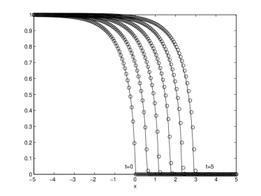
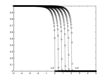
We consider the following generalization of the Fisher-Kolmogoroff equation (10)

$$\frac{\partial{u}}{\partial{t}}=u^{p}(1-u^{q})+\frac{\partial{}}{\partial{x}}\left(u^{m}\frac{\partial{u}}{\partial{x}}\right)$$ (10)

The existence of travelling waves can be proved for a wide range of parameters $p,q,m$ [Mur02]. For example in the paper [New83] gives the expression of such a wave for the case $p=1$ and $q=m=\alpha$. The speed $c$ and the exact solution are:

$$c=\frac{1}{\sqrt{1+\alpha}}\qquad u(t,x)=\left[\left(1-e^{\frac{\alpha(x-ct)}{\sqrt{1+\alpha}}}\right)^{\frac{1}{\alpha}}\right]_{+}$$ (11)

Figure 1 shows the numerical solutions obtained for $t=5$, using $300$ points in the interval $x\in[-5,5]$. The initial data and the exact solutions shown are defined according to (11). The accuracy of the schemes is good in both cases. In the case with $\alpha=5$ there is a lower accuracy around the corner, due to the higher degeneracy of the diffusion term and the more pronounced stiffness of the reaction term.

Table 2 shows the errors and convergence rates, measured at $t=5$, comparing the results of the schemes presented in this paper and those obtained with the schemes described in [CNPS07]. In order to apply the schemes of [CNPS07], equation (10) was rewritten in the “conservative form” $u_{t}=[u^{m}/m]_{xx}+u(1-u^{\alpha})$, where $m=\alpha+1$. We point out that, although we employed the Heun scheme and ENO reconstruztions of order $3$, the convergence rate is limited by the $C^{(0)}$ regularity of the solution. The comparison shows that the schemes for the conservative form perform slightly better than those described here for the nonconservative form, both regarding the convergence rate and the absolute value of the errors. Both schemes could be improved by integrating the reaction term with the diagonnally implicit part of the IMEX scheme, expecially in the test with $\alpha=5$.

Thus, whenever the equation can be put in the conservative form required by the schemes of [CNPS07], those are to be preferred. In the other cases, which frequently occour in more than one dimensions or in the case of systems of equations, the present scheme is a good choice for the numerical integration of the differential problem.

	$\alpha=2$				$\alpha=5$
	Section 3		[CNPS07]		Section 3		[CNPS07]
$N$	$\|E\|_{2}$	rate	$\|E\|_{2}$	rate	$\|E\|_{2}$	rate	$\|E\|_{2}$	rate
30	2.3515e-01		6.9686e-02		4.5251e-01		5.0452e-02
60	6.9899e-02	-1.75	4.7352e-03	-3.87	2.0266e-01	-1.15	2.7865e-02	-0.85
120	2.4679e-02	-1.50	4.1303e-03	-0.19	9.0192e-02	-1.16	1.3893e-02	-1.00
240	6.0385e-03	-2.03	7.0980e-04	-2.54	3.2529e-02	-1.47	3.1202e-03	-2.15
480	2.1158e-03	-1.51	3.2753e-04	-1.11	1.2977e-02	-1.32	1.1481e-03	-1.44
avg. rate		-1.71		-1.82		-1.28		-1.40

Table 2: Errors and convergence rates on the travelling wave solution (11). For $\alpha=2$ and $\alpha=5$ we compare the results of the schemes proposed in this paper with those described in [CNPS07]. The last row is the average convergence rate.

4.3 Two dimensional tests

Figure 2: Initial data (top) and supports (bottom) of the numerical solution of (12) at different times.

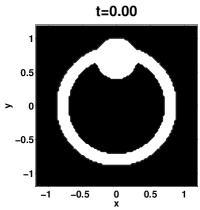
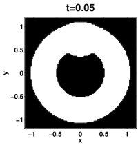
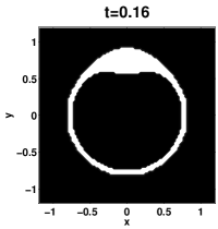
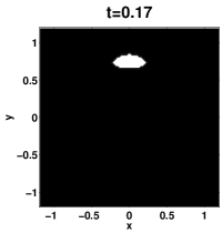
We tested the multi-dimensional version of our integration scheme on the equation

$$\frac{\partial{u}}{\partial{t}}=\mathrm{\Delta}(u^{m})-cu^{p}$$ (12)

for $x\in[-2,2]^{2}$ and $t\geq 0$. The above equation presents interesting finite-time extinction phenomena, reported in [Mik95].

We tested the ability to reproduce the extinction phenomenon and the persistence of asymmetry in the initial datum along the evolution. We took $u(x,y,0)$ as a radially symmetric function with a small perturbation, see Figure 2, and evolved it with the same equation and parameters as before, until extinction. Figure 2 shows clearly that the initial perturbation of the radial symmetry is maintained until the solution vanishes.

4.4 Application to a system of PDEs

Figure 3: Model (13) for frog populations in [TLB07b]. Solutions at $t=0.5$, $t=5$, $t=5.5$, $t=10$, $t=15$ and $t=20$. Note the different scale in the top right panel. In blue: the $u$ population released at $x=0$ at $t=0$; in green: the $v$ population, that is released at $x=0$ after the first has settled ($t=5$ here). The black dashed line is the total settled population, i.e. $u_{s}+v_{s}$.

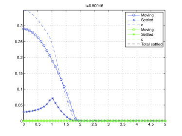
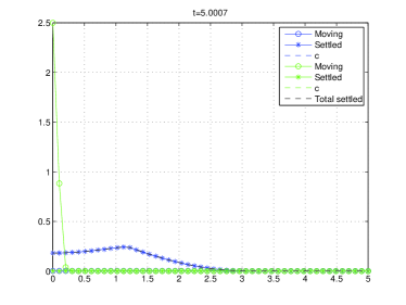
We consider now an ecological model described in [TLB07b]. It consists in a system of PDEs describing the dispersal and settling of frogs. The model splits the population of frogs in two classes: the ones that have already settled and those that are still migrating. The moving class diffuses with rate $D$ and settles at rate $S$. Once an individual is in the settled class, they cannot migrate any more. The authors of [TLB07b] study various mechanisms of dispersal and settling: we describe here only those that they think relevant in the case study considered in the paper, that is density-dependent dispersal and constant or $u$-dependent settling rate.

Let $$u_{m}(t,x) u_{s}(t,x) D(u) S(u)$$ and be the population density of migrating and settled animals, and suitable functions describing the dispersal and settling mechanism. The population is described by the following parabolic equations.

$$\frac{\partial{u_{m}}}{\partial{t}} =\mu\nabla_{x}\cdot\left(D(u_{m}+u_{s})\nabla_{x}(u_{m})\right)-S(u_{m}+u_{s})u_{m}$$ (13a)

$$\frac{\partial{u_{s}}}{\partial{t}} =S(u_{m}+u_{s})u_{m}$$ (13b)

Initial conditions mimic a population concentrated around $$x=0 u_{m}(0,x) u_{s}(0,x)=0 D(u)=u/u_{0} u_{0} u_{m}$$ for and . In the case (for constant ) considered in the paper, the diffusion equation (13a) is degenerate and gives rise to Barenblatt-like profiles for the density of the moving population. We point out that a very accurate numerical approximation is very important, since there is no mechanism in the model to move the population once it has settled.

If a second population $v$ is released in the same spot, the model is augmented with the following equations:

$$\frac{\partial{c_{u}}}{\partial{t}} =\alpha\mathrm{\Delta}_{x}(c_{u})+\beta(u_{m}+u_{s}-c_{u})$$ (13c)

$$\frac{\partial{v_{m}}}{\partial{t}} =\mu\nabla_{x}\cdot\left(D(v_{m}+v_{s})\nabla_{x}(v_{m})\right)+\gamma\nabla_{x}\cdot\left(v_{m}\nabla_{x}(c_{u})\right)-S(u_{s}+v_{m}+v_{s})v_{m}$$ (13d)

$$\frac{\partial{v_{s}}}{\partial{t}} =S(u_{s}+v_{m}+v_{s})u_{m}$$ (13e)

Here $v_{m}$ and $v_{s}$ are the densities of migrating and settled animals belonging to the second population, while $c_{u}$ is a diffusible pheromone released by the first population and discouraging the $v$ population from staying in the area where the $u$ density is higher.

The case study of [TLB07b] is about a release of a batch of frogs ($v$) at the same spot where an earlier release ($u$) had taken place, at a time when the frogs from the first batch have already settled down. In order to reproduce the situation of the case study of [TLB07b], one has to evolve in time the system (13) starting with an initial nonzero $u_{m}$ population while $u_{s}=v_{m}=v_{s}=0$ and adding a nonzero $v_{m}$ density after the $u$ population had time to settle settled (that is when $u_{m}$ is negligible).

We employed free-flow boundary conditions and chose parameters as suggested in [TLB07a]:

$$\mu=1\qquad\gamma=0\qquad\alpha=0.01\qquad\beta=10\qquad$$

The initial population is taken to be

$$u_{m}(0,x)=2.5e^{-100x^{2}}$$

and we chose

$$D(u)=\frac{u}{0.25}\qquad S(u,c)=\chi\left(1-\frac{u}{0.25}\right)$$

where $\chi(x)=1$ when $x>0$ and $\chi(x)=0$ otherwise.

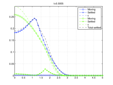
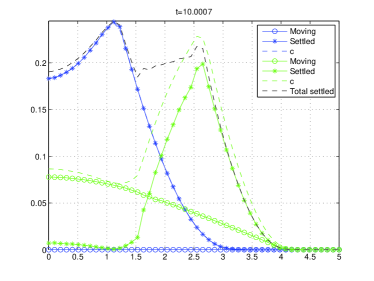
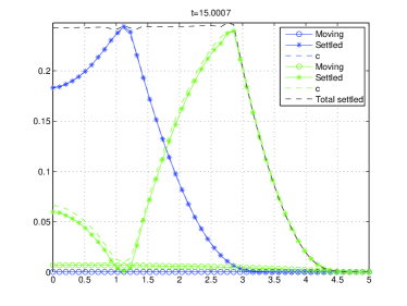
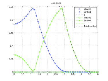
The $u$ population settles in the time lapse from $t=0$ to $t=5$ with maximum density located some distance apart from the original release spot ($x=0$ in the simulation). After this, the release of the second batch is simulated setting, at $t=5$, $v_{m}(5,x)=u_{m}(0,x)$. Thus the same initial condition is employed for both batches.

Figure 3 clearly shows that this second population first moves further away than the peak of the $u_{s}$ distribution and start settling there. Only afterwards the $v$ population settles also near $x=0$.

The panel in figure 3 shows the evolution of the system, from the early $u$ dispersal that gives rise to a Barenblatt-like profile for $u_{m}$ (upper left), to the release of the $v$ population when $u_{m}\simeq 0$ (upper right), the early migration and settling of the second population around $x=2$ (middle), the beginning of the secondary settling at $x=0$ (bottom left) and the final steady state (bottom right).

We reproduced with our method also all the other cases studied in [TLB07a]. We point out that the standard integration procedure used for the simulations in [TLB07a] required a smoothing of the $\chi$ function and, despite that, produces unrealistic wiggles in the population densities, that are not seen with the method presented here.

5 Conclusions

We have proposed and analyzed relaxed schemes for nonlinear degenerate reaction diffusion equations. By using suitable discretization in space and time, namely ENO/WENO non-oscillatory reconstructions for numerical fluxes and IMEX Runge-Kutta schemes for time integration, we have obtained a class of high order schemes. The theoretical convergence analysis for the semidiscrete scheme and the stability for the fully discrete schemes have been studied by us, for the case of nonlinear diffusion, in [CNPS07].

Here we tested these schemes on travelling waves solutions and in cases where the solution vanishes in finite time. In all cases we observed a very good agreement with known properties of the exact solutions.

Moreover we have shown how the accurate approximation of the fronts arising in degenerate parabolic equations can lead to improved accuracy in the simulation of an ecologically relevant model.

References

- [Aro70] D. G. Aronson. Regularity properties of flows through porous media: a counterexample. SIAM J. Appl. Math., 19:299–307, 1970.
- [ARS97] U. Asher, S. Ruuth, and R.J. Spiteri. Implicit-explicit Runge-Kutta methods for time dependent Partial Differential Equations. Appl. Numer. Math., 25:151–167, 1997.
- [CNPS07] F. Cavalli, G. Naldi, G. Puppo, and M. Semplice. High-order relaxation schemes for non linear degenerate diffusion problems. SIAM Journal on Numerical Analysis, 45(5):2098–2119, 2007.
- [GRSGM00] G. Garcia-Ramos, F. Sanchez-Garduno, and P. K. Maini. Dispersal can sharpen parapatric boundaries on a spatially varying environment. Ecology, 81(3):749–760, 2000.
- [HNW93] E. Hairer, S. P. Nørsett, and G. Wanner. Solving ordinary differential equations. I, volume 8 of Springer Series in Computational Mathematics. Springer-Verlag, Berlin, second edition, 1993. Nonstiff problems.
- [JX95] S. Jin and Z. Xin. The relaxation schemes for systems of conservation laws in arbitrary space dimensions. Comm. Pure and Appl. Math., 48:235–276, 1995.
- [KC03] Christopher A. Kennedy and Mark H. Carpenter. Additive Runge-Kutta schemes for convection-diffusion-reaction equations. Appl. Numer. Math., 44(1-2):139–181, 2003.
- [Mik95] K. Mikula. Numerical solution of nonlinear diffusion with finite extinction phenomenon. Acta Math. Univ. Comenian. (N.S.), 64(2):173–184, 1995.
- [Mur02] J. D. Murray. Mathematical biology. I, volume 17 of Interdisciplinary Applied Mathematics. Springer-Verlag, New York, third edition, 2002. An introduction.
- [Mur03] J. D. Murray. Mathematical biology. II, volume 18 of Interdisciplinary Applied Mathematics. Springer-Verlag, New York, third edition, 2003. Spatial models and biomedical applications.
- [New83] William I. Newman. The long-time behavior of the solution to a nonlinear diffusion problem in population genetics and combustion. J. Theoret. Biol., 104(4):473–484, 1983.
- [NP98] G. Naldi and L. Pareschi. Numerical schemes for kinetic equations in diffusive regimes. Appl. Math. Lett., 11(2):29–35, 1998.
- [NP00] G. Naldi and L. Pareschi. Numerical schemes for hyperbolic systems of conservation laws with stiff diffusive relaxation. SIAM J. Numer. Anal., 37:1246–1270, 2000.
- [PR05] L. Pareschi and G. Russo. Implicit-explicit Runge-Kutta schemes and applications to hyperbolic systems with relaxation. J. Sci. Comp., 25:129–155, 2005.
- [SO89] C. Shu and S. Osher. Efficient implementation of essentially nonoscillatory shock-capturing schemes. II. J. Comput. Phys., 83(1):32–78, 1989.
- [TLB07a] Abbey J. Trewenack, Kerry A. Landman, and Ben D. Bell. Dispersal and settling of translocated populations: a general study and a New Zealand amphibian case study. J. Math. Biol., 55(4):575–604, 2007.
- [TLB07b] Abbey J. Trewenack, Kerry A. Landman, and Ben D. Bell. Dispersal and settling of translocated populations: a general study and a New Zealand amphibian case study. J. Math. Biol., 55(4):575–604, 2007.