Athena: A New Code for Astrophysical MHD
Abstract
A new code for astrophysical magnetohydrodynamics (MHD) is described. The code has been designed to be easily extensible for use with static and adaptive mesh refinement. It combines higher-order Godunov methods with the constrained transport (CT) technique to enforce the divergence-free constraint on the magnetic field. Discretization is based on cell-centered volume-averages for mass, momentum, and energy, and face-centered area-averages for the magnetic field. Novel features of the algorithm include (1) a consistent framework for computing the time- and edge-averaged electric fields used by CT to evolve the magnetic field from the time- and area-averaged Godunov fluxes, (2) the extension to MHD of spatial reconstruction schemes that involve a dimensionally-split time advance, and (3) the extension to MHD of two different dimensionally-unsplit integration methods. Implementation of the algorithm in both C and Fortran95 is detailed, including strategies for parallelization using domain decomposition. Results from a test suite which includes problems in one-, two-, and three-dimensions for both hydrodynamics and MHD are given, not only to demonstrate the fidelity of the algorithms, but also to enable comparisons to other methods. The source code is freely available for download on the web.
1 Introduction
Numerical methods are essential for the study of a very wide range of problems in astrophysical fluid dynamics. As such, the development of more accurate and more capable algorithms, along with a description of their implementation on modern parallel computer systems, is important for progress in the field. This paper describes a new code for astrophysical magnetohydrodynamics (MHD) called Athena, developed through a collaborative effort between the authors.
There are many numerical algorithms available for solving the equations of compressible MHD. One of the most successful is based on operator splitting of the equations, with higher-order upwind methods used for the advection terms, centered-differencing for the remaining terms, and artificial viscosity for shock capturing. This algorithm, as implemented in for example the ZEUS code (Stone & Norman 1992a; b; Clarke 1996; Hayes et al. 2006), has been used for many hundreds of applications in astrophysics. The key advantage of the method is its simplicity, making it easy to extend with more complex physics (for example, Stone & Norman 1992c; Turner & Stone 2001; De Villiers & Hawley 2003, Hayes & Norman 2003).
However, in the fifteen years since the development of ZEUS, static and adaptive mesh refinement (SMR and AMR respectively) have emerged as powerful techniques to resolve a large range in length scales with grid-based methods. Berger & Colella (1990) have shown that in order to prevent spurious reflections, it is important to enforce conservation at internal boundaries between fine and coarse meshes. Thus, operator-split methods that do not solve the dynamical equations in conservation form such as ZEUS are unsuitable for use with SMR or AMR. This has been our primary motivation for the development of Athena.
The numerical algorithms in Athena are based on directionally-unsplit, higher-order Godunov methods, which not only are ideal for use with both SMR and AMR, but also are superior for shock capturing and evolving the contact and rotational discontinuities that are typical of astrophysical flows. Athena is neither the first nor the only MHD code based on these methods which is designed for use with AMR; others include RIEMANN (Balsara 2000), BATS-R-US (Powell et al. 1999; Gombosi et al. 2004), AMRVAC (Tóth 1996; Nool & Keppens 2002), Nirvana (Ziegler 2005), RAMSES (Fromang et al. 2006), PLUTO (Mignone et al. 2007), and AstroBEAR (Cunningham et al. 2007). While the wealth of papers describing AMR MHD codes demonstrates the interest in and importance of these numerical methods, it also calls into question the need for another paper describing yet another code. However, it has been our experience that the precise details of the algorithm can be important. The numerical methods in Athena differ, sometimes in small ways, and sometimes in substantial ways, from those in other codes. Our goals in developing Athena have been to write an accurate, easy-to-use, adaptable, and maintainable code. Our hope is that the comprehensive description provided in this paper will be useful to anyone who adopts, modifies, or builds upon the code, as well as for others developing their own codes.
The development of Godunov methods for MHD has required substantial progress over the past decade. Most of the effort has focused on two main areas: the multidimensional integration algorithm, and the method by which the divergence-free constraint on the magnetic field is enforced. Different options have been explored in different combinations, including unconstrained directionally split integrators (Dai & Woodward 1994), or directionally split and unsplit integrators that use either a Hodge projection to enforce the constraint (Zachary et al. 1994; Ryu et al. 1995; Balsara 1998; Crockett et al. 2005), a non-conservative formulation that allows propagation and damping of errors in the constraint (Powell 1994; Falle et al. 1998; Powell et al. 1999; Dedner et al. 2002), or some form of the constrained transport (CT) algorithm of Evans & Hawley (1988) to enforce the constraint (Dai & Woodward 1998; Ryu et al. 1998; Balsara & Spicer 1999; Tóth 2000, hereafter T2000; Pen et al. 2003; Londrillo & Del Zanna 2004; Ziegler 2004; Fromang et al. 2006; Mignone et al. 2007; Cunningham et al. 2007). T2000 provides a systematic comparison of many of these techniques using an extensive test suite.
While the algorithms in Athena build upon this progress, they also incorporate several innovations, including (1) the extension of two different directionally unsplit integration algorithms to MHD, including the corner transport upwind (CTU) method of Colella (1990 – hereafter the CTU+CT algorithm), and a simpler predictor-corrector method (see the appendix in Falle 1981) similar to the MUSCL-Hancock scheme described by van Leer (2006; Toro 1999 – hereafter referred to as the VL+CT algorithm), (2) the method by which the Godunov fluxes are used to calculate the electric fields needed by CT, and (3) the extension of the dimensionally-split spatial reconstruction scheme in the piecewise parabolic method (PPM) of Colella & Woodward (1984, hereafter CW) to multidimensional MHD. The mathematical foundations of these ingredients for integration in two dimensions (2D) is presented in detail in Gardiner & Stone (2005, hereafter GS05), and for three dimensions (3D) in Gardiner & Stone (2008, hereafter GS08). The focus of this paper is on the implementation rather than the mathematics of the methods.
The use of two distinct unsplit integration algorithms in Athena, namely the CTU+CT and the VL+CT algorithms, allows us to compare the advantages and disadvantages of both. We find the CTU+CT algorithm is generally less diffusive and more accurate than VL+CT. Thus, for simplicity sake, the description in this paper will be based on the CTU+CT algorithm. However, for some applications the VL+CT algorithm has definite advantages. A complete description of the 3D VL+CT algorithm implemented in Athena, including the results of tests in comparison to the CTU+CT algorithm, is provided in a short companion paper (Stone & Gardiner 2008, hereafter SG08).
The primary goal of this paper is to provide a comprehensive description of Athena that will serve as a reference for others to adopt, modify, and extend the code for their own research. As with ZEUS, the source code is freely available from the web, along with documentation and an extensive set of test problems that are useful for any method. The organization of this paper is as follows: §2 introduces the equations of motion solved by Athena, while §3 describes their finite-volume and finite-area discretizations. Sections 4-6 describe in detail the numerical algorithms in one, two, and three spatial dimensions respectively, including details such as the reconstruction algorithm, Riemann solvers used to compute upwind fluxes, and the unsplit CTU+CT integrator used in multidimensions. In §7 the implementation of the algorithms in both C and Fortran95 on parallel computer systems is discussed. The results of a comprehensive test suite composed of problems in 1D, 2D, and 3D are given in §8. Finally, we summarize and discuss future extensions to the code in §9.
2 Basic Equations
Athena implements algorithms which solve the equations of ideal MHD, which can be written in conservative form as
| (1) | |||||
| (2) | |||||
| (3) | |||||
| (4) |
where is a diagonal tensor with components (with the gas pressure), is the total energy density
| (5) |
and . The other symbols have their usual meaning. These equations are written in units such that the magnetic permeability .
An equation of state appropriate to an ideal gas, (where is the ratio of specific heats, and is the internal energy density), has been assumed in writing equation 5. For a barotropic equation of state (for example, , where is the isothermal sound speed), both equations 3 and 5 are dropped from the system. Of course, in this case total energy is not conserved. The algorithms implemented in Athena can solve the equations of motion in four regimes: both hydrodynamics or MHD with either an ideal-gas or barotropic equation of state. In each regime the system of equations to be solved is different in number and form, however the same general numerical techniques apply. Extension of the numerical methods to a more complex, e.g. tabular, equation of state is possible.
It is useful to define vectors of the conserved and primitive variables, and respectively, with components in Cartesian coordinates (for adiabatic MHD)
| (6) |
where is the momentum density. The conservation laws can now be written in a compact form (in Cartesian coordinates)
| (7) |
where , , and are vectors of fluxes in the , , and directions respectively, with components
| (8) |
| (9) |
| (10) |
Extension to curvilinear coordinates requires adding metric scale factors to the definitions of the fluxes, or using a non-conservative formulation that treats grid curvature as source terms, or a combination of these approaches.
For hydrodynamics, or for a barotropic equation of state (or for both), the appropriate components of the vectors , , and their fluxes are dropped. While the last three components of these vectors represents the induction equation in Cartesian coordinates, the numerical algorithm actually used to evolve the magnetic field is very different in comparison to that used for the other components, as described in the next section.
3 Discretization
Athena integrates the equations of motion on a regular, three-dimensional Cartesian grid. The continuous spatial coordinates () are discretized into () cells within a finite domain of size () in each direction respectively. The cell denoted by indices () is centered at position (). For simplicity we describe the algorithm with the assumption that the sizes of the grid cells in each direction, , , and respectively, are uniform throughout the domain; the numerical methods are easily extended to non-uniform grids.
Time is discretized into non-uniform steps between the initial value and the final stopping time . Following the usual convention, we use a superscript to denote the time level, so . Hereafter we drop the superscript on with the understanding that the time step may vary.
3.1 Mass, Momentum, and Energy: Finite-Volumes
Discretizations based on the integral, rather than the differential, form of equations 1 through 4 have numerous advantages for flows that contain shocks and discontinuities (LeVeque 2002). Integration of equation 7 over the volume of a grid cell, and over a discrete interval of time gives, after application of the divergence theorem,
| (11) | |||||
where
| (12) |
is a vector of volume-averaged variables, while
| (13) |
| (14) |
| (15) |
are vectors of the time- and area-averaged fluxes. We use the convention here, and throughout this paper, that half-integer subscripts denote the edges of the computational cells, that is is the location of the interface between the cells centered at and . Thus, the fluxes are evaluated at (and are normal to) the faces of each grid cell (see figure 1). Note the half-integer superscript on the fluxes denote a time average, rather than representing the flux evaluated at .
As has been pointed out by many previous authors, equations 11 through 15 are exact: to this point no approximation has been made. A numerical algorithm for MHD within the finite-volume approach requires accurate and stable approximations for the time- and area-averaged fluxes defined by equations 13 through 15. In principle, one can approximate the fluxes to any order of accuracy, although in practice most algorithms are restricted to second-order. A variety of authors are exploring the use of higher than second-order accurate time- and spatial integration (Londrillo & Del Zanna 2000), especially in the context of WENO schemes (Balsara & Shu 2000; McKinney et al. 2007). Higher-order schemes improve the accuracy primarily in smooth flow, not in shocks or discontinuities, and are more difficult to combine with AMR. Based on a set of 1D hydrodynamic test problems, Greenough & Rider (2003) conclude that a second-order Godunov scheme provides more accuracy per computational cost than a fifth-order WENO scheme. Although it is clear that higher-order schemes will have advantages for some applications, in Athena we shall restrict ourselves to second-order accuracy in both space and time.
3.2 Magnetic Field: Finite-Areas
The last three components of equations 11 through 15 are the finite-volume form of the induction equation, which could be used to integrate the volume-averaged components of the magnetic field. Instead, in Athena we use an integral form of the induction equation that is based on area- rather than volume-averages. In GS05, we have argued that area-averaging is the most natural representation of the integral form of the induction equation. This form conserves the magnetic flux through each grid cell, and as a consequence automatically preserves the divergence free constraint on the field (Evans & Hawley 1988).
Integration of equation 4 over the three orthogonal faces of the cell located at (), () and () respectively, gives
| (16) | |||||
| (17) | |||||
| (18) | |||||
where
| (19) |
| (20) |
| (21) |
are the area-averaged components of the magnetic field centered on each of these faces, and
| (22) |
| (23) |
| (24) |
are the components of the electric field (the electromotive force, or emf) averaged along the appropriate line element. Note this discretization requires a staggered grid, that is the area-averaged components of the magnetic field are located at the faces (not the centers) of the cells. Figure 1 shows the relative locations of the cell-centered volume-averaged variables (), the face-centered area-averaged components of the magnetic field () the face-centered area-averaged fluxes (), and the edge-centered line-averaged emfs (, etc.)..
There are many advantages to using a discretization of the induction equation based on area- rather than volume-averages (GS05). The most important is that the finite-volume representation, i.e. the cell-volume average, of the divergence-free constraint constructed using the time-advanced field
| (25) | |||||
is kept zero by the discrete form of the induction equation, equations 16 through 18, provided of course it was zero at (Evans & Hawley 1988). Equivalently, the CT algorithm conserves the magnetic flux through each grid cell. The most serious disadvantage of using CT with face-centered fields is that it complicates the implementation of the algorithm, and the interface to AMR drivers.
Of course, there are many possible discretizations of the divergence-free constraint, and the CT algorithm based on face-centered fields described above preserves only one of them (equation 25). T2000 has described an extension to CT which preserves the constraint formulated using several different discretizations of the divergence operator based on cell-centered fields. It is difficult to assess, for a given integration algorithm, whether preserving one discretization is more important than any other. We have argued (GS05; GS08) that the discretization based on face-centered fields is more consistent with the finite volume approach in that it conserves the magnetic flux within each individual grid cell, equivalently it conserves the volume integral of the density of magnetic monopoles at the level of grid cells. In addition, in GS08 (see also §8) we describe a simple test problem based on the advection of a field loop that is sensitive to whether the discretization of the divergence-free constraint that is preserved is consistent with the numerical algorithm used to update the induction equation. If not, growth of net magnetic flux will be observed.
In Athena, the primary description of the magnetic field is taken to be the face-centered area-averages equations 19 through 21. However, cell-centered values for the field are needed to construct the fluxes of momentum and energy (equations 8 through 10). Here, we adopt the second-order accurate averages
| (26) |
| (27) |
| (28) |
Operationally, the face-centered fields are evolved using equations 16 through 18, and at the end of each integration step the cell-centered fields are computed using equations 26 through 28. As shown in GS05 (and discussed further in §5.3), the relationship between the face- and cell-centered components of the field given above determines how their fluxes (the time- and line-averaged emfs in equations 22 through 24 and last three components of the time- and area-averaged fluxes in equations 13 through 15 respectively) are computed from one another.
4 One-dimensional integration algorithm
It is useful (and standard) pedagogy to describe the algorithm for integration of the equations of motion in 1D first, before introducing methods for multidimensions. However, for MHD, this approach can be misleading. In 1D the divergence-free constraint reduces to the condition that the longitudinal component of the magnetic field be constant, the CT algorithm is not needed, and the discrete forms of the induction equation for the area- and volume-averaged fields are identical. As a consequence, 1D algorithms for MHD are a simple extension of those for hydrodynamics. Moreover, 1D test problems for MHD will not reveal errors associated with the development of a non-solenoidal field. Any rigorous test suite for MHD must be based on multidimensional problems.
Nonetheless, we begin a description of the algorithms in Athena with the 1D integrator as it allows us to introduce basic components, such as Riemann solvers and methods for spatial reconstruction, required in multidimensions. We emphasize that the integrators for 2D and 3D MHD, described in detail in §5 and §6 respectively, are substantially different and more complex than the 1D integrator introduced here.
In 1D, the equations of adiabatic MHD can be written in Cartesian coordinates as
| (29) |
where the vectors of conserved variables and their fluxes are
| (30) |
Note these are identical to equations 6 and 8 with the sixth component dropped. We introduce the notation that vectors denoted by lower-case letters are in one spatial dimension (and therefore contain 7 components for adiabatic MHD, rather than 8 for the same vectors written in full 3D). It is important to remember that the components of the 1D vectors defined in equation 30 will change depending on direction. For example, in the direction for ideal MHD, the order of the three components are permuted (so the second to fourth components become , , and respectively), and the sixth and seventh components become and respectively.
The finite-volume discretization of equation 29 proceeds as described in §3.1, giving
| (31) |
where
| (32) |
is a vector of volume-averaged variables, while
| (33) |
are the time-averaged fluxes at the interface located at .
In a Godunov method, the time-averaged fluxes (equation 33) are computed using a Riemann solver (see Toro 1999 for an introduction to the subject). Figure 2 illustrates the process (see also LeVeque 2002). Starting from the 1D volume-averages stored at cell-centers a spatial reconstruction scheme is used to construct the conserved quantities to the left- and right-sides of the interface, and respectively. For the CTU+CT integrator, the reconstruction is performed in the primitive variables, and includes a time-advance using characteristic variables, with and computed from the resulting interpolants (this step will be described in detail in §4.2). Due to the slope-limiters used to keep the interpolants non-oscillatory, the left- and right-states and will not be equal, except in smooth flow. Thus, they define a Riemann problem, the solution to which is the time evolution of the various waves, and the intermediate states that connect them, that propagate away from the interface. The solution to the Riemann problem, evaluated at the location of the interface, can be used to construct the time-averaged flux (details of the calculation of fluxes using Riemann solvers is given in §4.3).
4.1 Steps in the 1D Algorithm
The 1D algorithm outlined above can be summarized by the following steps:
Step 1. From , the volume averages at time level , compute the left- and right-states and at every interface using one of the spatial reconstruction algorithms described below in §4.2.
Step 2. Compute the time-averaged fluxes at every interface using one of the Riemann solvers described in §4.3. Note the face-centered longitudinal component of the magnetic field is passed to the Riemann solver as a parameter.
Step 3. Update the cell-centered conserved variables and the transverse components of the magnetic field using the finite-volume difference equation in 1D, equation 31.
Step 4. Increment the time: . Compute a new timestep that satisfies an estimate of the CFL stability condition based on wavespeeds at cell centers
| (34) |
where is the CFL number, is the fast magnetosonic speed in the direction, evaluated using the updated quantities, and the maximum is taken over all grid cells. Note this is only an estimate of the CFL stability condition, since the wavespeeds used in the Riemann solver can be different from those computed from the cell-centered values.
Step 5. Repeat steps 1-4 until the stopping criterion is reached, i.e..
The entire 1D integration algorithm is summarized by the flow chart shown in figure 3.
4.2 MHD Interface States
The first step in the 1D algorithm is to compute the left- and right-states and that define the Riemann problem at the interface located at . (Note that in our notation the left-state is actually on the right side of the cell center at , while the right-state is on the left side of the cell center at , see figure 2). The reconstruction is inherently 1D, and therefore is based on the vector of conserved variables in 1D (equation 30). This vector contains only the transverse components of the field: in 1D these are cell-centered quantities. For reconstruction in multidimensions, the cell-centered averages of the face-centered transverse components of the field (for example, equations 27 and 28 for reconstruction in the direction) would be used. When the longitudinal component of the field is needed, the area-averaged value stored at the appropriate interface is adopted. The fact that the longitudinal component of the field does not need to be reconstructed from cell-centered values is a further advantage of the CT algorithm based on staggered (face-centered) fields; it avoids the problem of the longitudinal component being discontinuous at the interface due to slope-limited reconstruction from cell centers.
When the CTU+CT unsplit integrator is used in Athena, the second- and third-order reconstruction algorithms described below include both spatial interpolation with slope-limiting in the characteristic variables, and a characteristic evolution of the linearized system in the primitive variables. We have found these steps help to make the reconstruction less oscillatory. However, they also require an eigenvalue decomposition of the linearized equations of motion in the primitive variables. Appendix A catalogs the eigenvalues and left- and right-eigenvectors for adiabatic and isothermal hydrodynamics and MHD in the primitive variables needed for this approach. For more complex physics (e.g., relativistic MHD) this eigenvalue decomposition may be difficult. One advantage of the VL+CT integrator described in SG08 is that it does not require a characteristic evolution in the reconstruction step. This avoids the need for an eigenvalue decomposition in the primitive variables, and therefore this integrator may be a better choice for more complex physics. The interface state algorithm used in the VL+CT algorithm is described more fully in SG08.
4.2.1 Piecewise constant (first-order) reconstruction
The simplest possible reconstruction algorithm is to assume the primitive variables are piecewise constant within each cell (implying the conserved variables are also piecewise constant), leading to the first-order method
| (35) | |||||
First-order reconstruction is far too diffusive for applications, however it is useful for testing, or in those circumstances when extra diffusion is in fact desired.
4.2.2 Piecewise linear (second-order) reconstruction
A better approximation is to assume the primitive variables vary linearly within each cell (meaning that the profile of the conserved variables within a cell may be steeper than linear). This approximation leads to the second-order reconstruction algorithm used with the CTU+CT unsplit integrator that is given by the following steps:
Step 1. Compute the eigenvalues and eigenvectors of the linearized equations in the primitive variables using , the cell-centered primitive variables in 1D (which differs from defined in equation 6 only in that it lacks the longitudinal component of the magnetic field). Explicit expressions for these are given in Appendix A.
Step 2. Compute the left-, right-, and centered-differences of the primitive variables
| (36) | |||||
(Note that in these equations the subscripts , , and refer to locations relative to the cell-center at .)
Step 3. Project the left, right, and centered differences onto the characteristic variables
| (37) | |||||
where is a matrix whose rows are the appropriate left-eigenvectors computed in Step 1.
Step 4. Apply monotonicity constraints to the differences in the characteristic variables, so that the characteristic reconstruction is total variation diminishing (TVD), e.g. see LeVeque (2002).
| (38) |
Step 5. Project the monotonized difference in the characteristic variables back onto the primitive variables
| (39) |
where is a matrix whose columns are the appropriate right-eigenvectors computed in Step 1.
Step 6. Compute the left- and right-interface values using the monotonized difference in the primitive variables
| (40) |
| (41) |
where and are the largest and smallest eigenvalues computed in Step 1 respectively, at the appropriate cell center. Note these values are at different cell faces, with () located to the right (left) of the cell center at .
Step 7. Perform the characteristic tracing, that is subtract from the integral performed in step 6 that part of each wave family that does not reach the interface in , using (CW; Colella 1990)
| (42) |
| (43) |
where the sums are taken only over those waves that propagate towards the interface (i.e., whose eigenvalue has the appropriate sign), and and are the rows and columns of the left- and right-eigenmatrices respectively corresponding to .
When using approximate Riemann solvers that average over intermediate states (like the HLL family of solvers), it is also necessary to include a correction for waves which propagate away from the interface in order to make the algorithm higher than first-order. This is because either the right-interface state (if the wavespeed is positive) or the left-interface state (if the wave speed is negative) will not include the half-timestep predictor evolution in the reconstruction, and will thus be first-order. Since the numerical flux in the HLL solver is given by a weighted average of the flux in the left-interface state and the right-interface state for such waves, the flux itself will be first-rder. Specifically, an additional term and is added to each of equations 42 and 43 respectively, where these terms are
| (44) |
| (45) |
We emphasize these terms are not added when the Roe or exact solvers are used.
Step 8. Finally, convert the left- and right-states in the primitive to the conserved variables, and .
4.2.3 Piecewise parabolic (third-order) reconstruction
Although the numerical algorithms in Athena are formally only second-order accurate, we have found that using third-order accurate spatial reconstruction can lower the amplitude of the truncation error and increase the accuracy of the solution. Thus, we have implemented the PPM interface state algorithm of CW in Athena. In §8, we provide a quantitative comparison of both the second-order (PLM) and third-order (PPM) reconstruction algorithms for smooth and discontinuous solutions in 1D, 2D and 3D.
The PPM reconstruction algorithm consists of the following steps.
Steps 1 through 5. These steps are identical to the first five steps in the second-order algorithm, see §4.2.2.
Step 6. Use parabolic interpolation to compute values at the left- and right-side of each cell center
| (46) |
where in the above, the subscript () refers to the left (right) side of cell center at .
Step 7. Apply further monotonicity constraints to ensure the values on the left- and right-side of cell center lie between neighboring cell-centered values (CW equation 1.10). These can be written as a series of conditional statements:
These conditions are applied independently to each component of .
Step 8. Compute the coefficients for the monotonized parabolic interpolation function,
| (47) |
Step 9. Compute the left- and right-interface values using monotonized parabolic interpolation (CW equation 1.12)
| (48) |
| (49) |
where and respectively, and and are the largest and smallest eigenvalues computed in Step 1 respectively. Note these values are at different cell faces, with () located to the right (left) of the cell center at .
Step 10. Perform the characteristic tracing, that is subtract from the integral performed in step 9 that part of each wave family that does not reach the interface in (CW; Colella 1990), using
| (50) |
| (51) |
where in the above
where the sums are taken only over those waves that propagate towards the interface (i.e., whose eigenvalue has the appropriate sign), and and are the rows and columns of the left- and right-eigenmatrices respectively corresponding to .
Once again, when using the HLL family of solvers, it is necessary to add a correction for waves which propagate away from the interface (as was required in step 7 of the PLM integration). These terms are identical to those in equations 44 and 45, which are correct to second-order. Again, we emphasize these terms are not added when the Roe or exact solvers are used.
Step 11. Finally, convert the left- and right-states in the primitive to the conserved variables, and .
An important ingredient of the reconstruction algorithm is the slope limiters used in steps 4 and 7. It is well-known that these limiters clip extrema in the solutions. We have also implemented the limiters described in Colella & Sekora (2007, hereafter CS), which are designed to prevent clipping of extrema. We find for some tests, the CS limiters significantly improve the solution compared to the original PPM limiters used above. For the test results shown in §8 we will always indicate if the CS limiters are used. The lesson, however, is that improving the convergence rate of the reconstruction algorithm is not always the best way to improve the overall accuracy of the solution.
4.3 Godunov Fluxes
The second step in the 1D algorithm is to compute time-averaged fluxes using a Riemann solver. Exact Riemann solvers for MHD (e.g. Ryu & Jones 1995) are generally too expensive for practical computations with current hardware. Moreover, since the full solution to the Riemann problem over all space-time is not required, but only the time-integral of the solution along the line (which gives the flux through the interface), approximate solvers which provide an accurate estimate of the flux are all that is needed. In fact, it is not even necessary to use the same solver to compute the flux at every interface in the grid. Instead, simple solvers can be used in smooth regions, while more robust (and expensive) solvers are adopted only when needed, for example in highly nonlinear flow where simple solvers fail (such as strong rarefactions). Since the latter generally occupy only a tiny fraction of the total number of interfaces over the whole grid, this strategy can be very cost effective.
A wide variety of approximate Riemann solvers for MHD are possible, including nonlinear solvers such as the HLL flux (Harten et al. 1983), the HLLD flux (Miyoshi & Kusano 2005), Toro’s FORCE flux (Toro 1999), Roe’s linear solver (Roe 1991) extended to MHD (Cargo & Gallice 1997), as well as MHD solvers based on other approximations (e.g, Dai & Woodward 1994; 1995; Zachary et al. 1994). A range of solvers is implemented in Athena, including exact solvers in the simplest cases (isothermal hydrodynamics). In the subsections below we describe some of the most useful.
Finally, it is important to emphasize that Godunov methods do not require expensive solvers based on complex characteristic decompositions. Simple solvers based on the local Lax-Friedrichs (LLF) or HLL fluxes that are typically adopted in other methods can also be used. Generally, the reason for adopting more complex and expensive Riemann solvers is that they reduce dissipation, especially in the neighborhood of discontinuities in the intermediate waves.
4.3.1 HLL Solvers
The simplest Riemann solver implemented in Athena uses the HLL fluxes as described by Einfeldt et al. (1991), hereafter termed the HLLE solver. The HLLE flux at the interface is defined as
| (52) |
where and are the fluxes evaluated using the left- and right-states of the conserved variables (using equation 30), and
| (53) |
| (54) |
Here and are the maximum and minimum eigenvalues of Roe’s matrix (see §4.3.2 and Appendix B), and are the velocity component normal to the interface in the left- and right-states respectively, and and are the maximum wavespeeds (the fast magnetosonic speed in MHD, or the sound speed in hydrodynamics) computed from the left- and right-states. The HLLE solver does not require a characteristic decomposition of the MHD equations; the eigenvalues of Roe’s matrix are given by simple, explicit formulae (see Appendix B). Note that if both and (or both and ), the HLLE flux will be (or ), as expected.
The HLLE solver approximates the solution to the Riemann problem using a single constant intermediate state computed from a conservative average, bounded using an estimate for the maximum and minimum wavespeeds. Thus, for hydrodynamics it neglects the contact wave, and for MHD it neglects the Alfvén, slow magnetosonic, and contact waves. For this reason, the HLLE is extremely diffusive for these waves (in fact, even if , contact discontinuities are diffused with the method). Thus, in practice, the HLLE solver is of limited use for applications. However, a distinct advantage of the HLLE solver is that the intermediate state is positive-definite, that is the pressure and density in the intermediate state can never be negative. Thus, in 1D it can be used to construct a positive-definite integration algorithm (Einfeldt et al 1991). This is in contrast to linearized solvers such as Roe’s method, in which the Riemann solver itself can produce negative densities and pressures for one or more of the intermediate states. The HLLE flux is therefore an excellent alternative in the rare circumstance that a more accurate solver fails. In multidimensions, however, use of the HLLE flux at higher than first order does not necessarily guarantee the method is positive definite: this depends on the details of the multidimensional integrator being used.
For hydrodynamics, the HLL solver has been extended to include the contact wave, resulting in a solution consisting of two constant intermediate states bounded by shocks and separated by a contact discontinuity. The resulting method is termed the HLLC solver. A basic description of the method is given in §10.4 of Toro (1999) and will not be repeated here; although it is important to note in Athena we choose the wavespeeds following the suggestion in Batten et al. (1997). This choice has the attractive property that the pressure in the intermediate states computed from the Rankine-Hugoniot relations across the left and right shocks is the same. We find that for hydrodynamics, this implementation of the HLLC solver produces results that are as, if not more, accurate than Roe’s method (see below), but at much lower computational cost. For 1D problems, it also is a positive definite method (although again, this is not guaranteed in multidimensions). Thus, the HLLC solver is highly recommended for adiabatic hydrodynamic simulations with Athena.
Recently, Miyoshi & Kusano (2005) have described an extension of the HLL solver to MHD which includes the fast magnetosonic, Alfvén, and contact waves. The resulting solver approximates the solution of the Riemann problem with four constant intermediate states. It reduces exactly to the HLLC solver when the longitudinal component of the magnetic field is zero, and is a positive definite method. The implementation of the solver is detailed in Miyoshi & Kusano (2005), and will not be repeated here. Tests using Athena indicate that this solver, termed HLLD, is typically as accurate as the MHD extension of Roe’s method, although it is much faster. Thus, the HLLD solver is the best choice for many MHD applications using Athena.
4.3.2 Roe’s Method
The HLL fluxes are based on an approximate solution to the nonlinear equations of MHD. Instead, Riemann solvers can be constructed from exact solutions to an approximate (linearized) form of the MHD equations, for example
| (55) |
The matrix is the Jacobian evaluated at some appropriate, constant mean state (treating this matrix as constant is what makes the system linear). Finding the exact solution to linear hyperbolic systems is less difficult because only discontinuities (no rarefactions) are allowed.
Of course, the challenge in developing linearized solvers is finding the appropriate representation for . Roe (1981) proposed one particularly useful linearization, which has subsequently been extended to adiabatic MHD by Cargo & Gallice (1997). In this linearization, the Jacobian is evaluated using an average state defined in the primitive variables as follows
| (56) | |||||
where is the enthalpy (used to compute the pressure), and the subscripts and denote the left- and right-states of each variable at the interface (computed using one of the reconstruction schemes described in §4.2). Explicit forms for the matrix , and its eigenvalues and eigenvectors for isothermal and adiabatic hydrodynamics and MHD are given in Appendix B.
Given the eigenvalues and left- and right-eigenmatrices and respectively, where denotes the characteristics in the solution, the Roe fluxes are simply
| (57) |
where as before , , and
| (58) |
| (59) |
and the and are the rows and columns of the left- and right-eigenmatrices corresponding to .
The primary advantage of Roe’s method is that it includes all of the characteristics in the problem, and therefore is less diffusive and more accurate than the HLLE solver for intermediate waves such as contact discontinuities. Moreover, Roe (1981) showed that it gives the flux exactly if the solution to the full nonlinear Riemann problem contains only an isolated discontinuity. However, because it is based on a linearization of the MHD equations, for some values of the left- and right-states Roe’s method will fail (Einfeldt et al. 1991); it will return negative densities and/or pressures in one or more of the intermediate states. In Athena, if this occurs we replace the calculation of the fluxes at that interface with the HLLE solver (which is a positive-definite method) or some other more accurate (e.g. an exact) solver. Tests indicate this is only required very rarely.
5 Two-dimensional integration algorithm
Probably the most popular method for constructing a 2D integration algorithm from the 1D method described in §4 is based on dimensional splitting (Strang 1968). Unfortunately, dimensional splitting cannot be used for MHD if the equations are to be solved in the conservative form. This is because during each one-dimensional update, only the transverse components of the magnetic field evolve (e.g., from equation 30 it is clear that is non-evolutionary during an update in the direction). However, the divergence-free constraint can only be maintained if all three components of the field evolve simultaneously. Thus, during the update in the direction, must evolve. The terms that describe this evolution cannot be written in conservative form, leading to for example the source term formulations of Powell (1994) and Powell et al. (1999). However, there are significant advantages to maintaining the conservative form (T2000), thus in Athena we adopt dimensionally-unsplit integrators for MHD, either based on the CTU+CT method (described below), or the VL+CT method (SG08). The use of directionally unsplit integrators in multidimensions is one of the most important components of the MHD algorithms in Athena.
Even after adopting an unsplit integration algorithm, combining it with the CT method to enforce the divergence-free constraint presents challenges. In particular, the method by which the corner-centered, line-averaged emfs are constructed from the face-centered, area-averaged fluxes returned by the Riemann solver is non-trivial. In GS05, we showed that simple arithmetic averaging does not work for the unsplit integrators adopted here. Instead, we developed several methods for constructing the emfs from the Godunov fluxes, the version actually used in Athena is described in §5.3. The resulting method reduces exactly to the 1D algorithm described in §4 for plane-parallel, grid-aligned flow, and preserves the flux normal to the plane of the calculation.
5.1 Steps in the 2D Algorithm
The 2D CTU+CT integration algorithm is based on the method of Colella (1990), and is described in detail in GS05; below we provide an overview of the main steps.
Step 1. Compute and store the left- and right-states at cell interfaces in both the direction () and the direction () simultaneously, using any of the 1D spatial reconstruction algorithms described in §4.2, for all the interfaces over the entire grid. Since the 1D reconstruction algorithms in Athena include a characteristic tracing step, when applied in multidimensions the 1D reconstruction must include source terms as described in §3.1 in GS05, and briefly in §5.2. Note that the components of (and ) are different on the and interfaces.
Step 2. Compute 1D fluxes of the conserved variables using any one of the Riemann solvers described in §4.3 at interfaces in both the and directions simultaneously
| (60) | |||||
| (61) |
where the appropriate longitudinal component of the magnetic field has been passed to the Riemann solver as a parameter.
Step 3. Using the algorithm of GS05, described in §5.3, calculate the emf at cell corners from the appropriate components of the face-centered fluxes returned by the Riemann solver in step 2, and the component of a cell center reference electric field calculated using the initial data at time level , i.e. .
Step 4 Evolve the left- and right-states at each interface by using transverse flux gradients. For example, the mass density, momentum density, energy density, and at the interface located at are advanced using
| (62) | |||||
| (63) |
Since the components of 1D vectors on the and interfaces differ, care must be taken to associate the components of the left- and right-states with the appropriate components of the transverse fluxes (for example, the components of with the components of ). The updates in equations 62 and 63 are directionally split (only the transverse flux gradient is used) and are based on the conservative form, therefore source terms must be added to the momentum density, energy, and . These are represented by the source term vector , the last term in both equations. For the left- and right-states on the interface, the source term vector has components where
| (64) | |||||
Expressions similar to equations 62 and 63 are used to update the interface states located at , that is and , for using the flux gradient in the direction. Source terms analogous to those in equation 64, but proportional to , also are necessary (see §4.1.2 in GS05). The in-plane components of the magnetic field are evolved using CT,
| (65) | |||||
| (66) |
using the emfs computed in step 3.
Step 5. Calculate a cell-centered reference electric field at , , which is needed as a reference state for the CT algorithm in step 7. The cell-centered velocities at the half-timestep needed to compute come from a conservative finite-volume update of the initial mass and momentum density, using the fluxes and . The cell-centered components of the magnetic field at the half-timestep come from averaging the face centered fields at the half-timestep computed by equations 65 and 66 in step 4 to cell-centers.
Step 6. Compute new fluxes at cell interfaces using the corrected left- and right-states from step 4 using one of the Riemann solvers described in §4.3, giving
| (67) | |||||
| (68) |
Note the appropriate face-centered fields updated to the half-timestep computed in step 4 are passed as parameters to the Riemann solver. If needed, the H-correction is used in this step to eliminate the carbuncle instability (see Appendix C).
Step 7. Apply the algorithm of §5.3 to calculate the CT electric fields using the numerical fluxes from step 6 and the cell center reference electric field calculated in step 5.
Step 8. Update the solution from time level to , using the 2D version of the finite-volume difference discretization (equation 11) for the mass density, momentum density, energy density, and , and the CT formulae (equations 16 and 17) for the in-plane components of the field and .
Step 9. Compute the cell-centered components of the magnetic field from the updated face-centered values using equations 26 and 27.
Step 10. Increment the time: . Compute a new timestep that satisfies an estimate of the CFL stability condition based on wavespeeds at cell centers
| (69) |
where is the CFL number, and are the fast magnetosonic speeds in the and directions respectively, evaluated using the updated quantities, and the minimum is taken over all grid cells. Note this is only an estimate of the CFL stability condition, since the wavespeeds used in the Riemann solver can be different from those computed from the cell-centered values.
Step 11. Repeat steps 1-10 until the stopping criterion is reached, i.e..
The entire 2D integration algorithm is summarized by the flow chart shown in figure 4.
5.2 MHD Interface States in 2D
In step 1 of the 2D algorithm discussed above, source terms must be added to the left- and right-states in the primitive variables that arise due to the characteristic tracing step in the reconstruction algorithms (see §4.2). These terms are necessary for a proper accounting of all the evolutionary terms that form the characteristic tracing step in multidimensioal MHD (see GS05 and GS08 for a complete discussion of the origin of these terms). Since the reconstruction is performed in the primitive variables, the only terms required are for the transverse components of the magnetic field (in contrast to step 4 in the 2D algorithm above, where the directional splitting is performed on the equations in conservative form, and therefore source terms were needed for , , and ). Thus, for the left-state at the interface located at , the change to the transverse fields due to the source term is
while for the left- and right-interface values at the interface located at , the change to the transverse field due to the source term is
Similar expressions are needed for the right-state values at each interface (GS05). In both cases the terms are added to the primitive variables after the reconstruction, and before converting back to the conserved variables.
5.3 Calculating the emfs
As discussed in §3, the CT update of the magnetic field requires the line-averaged emfs at cell corners, whereas the Riemann solver returns area-averaged electric fields at cell faces. For example, figure 5 shows the relative positions of the fluxes returned by the Riemann solver, and the emfs needed by CT, for the 2D grid cell with indices . In GS05, it was shown that the relationship between the two is determined by the averaging formulae used to convert between the face-centered area-averages of the magnetic field, and the cell-centered volume-averages. A variety of different algorithms were explored, and the best compromise between accuracy and simplicity was found to be
| (70) | |||||
where the derivative of on each grid cell face is computed by selecting the “upwind” direction according to the contact mode, e.g.
| (71) |
(where the subscript has been suppressed) with an analogous expression for the . The derivatives of the electric field in equation (71) are computed using the face centered electric fields (Godunov fluxes) and a cell center “reference” value , e.g.
| (72) |
where the cell center reference electric field is computed at the appropriate time level (either for step 3 of the 2D algorithm, or for step 7). To help clarify the above, figure 5 diagrams the relative locations of the Godunov fluxes, corner-centered emf, cell-centered reference states, and the derivatives of the electric field. Further details are provided in GS05 (and GS08 for the 3D case).
6 Three-Dimensional Integration Algorithm
The extension of the dimensionally unsplit CTU integrator due to Colella (1990) used in Athena from 2D to 3D is in fact quite complex. In particular, for stability with a CFL number requires 12 Riemann solves per cell per timestep, and multiple fractional timesteps are required to correct the left- and right-states with transverse flux gradients in a genuinely multidimensional fashion. This extension of CTU to 3D has been described by Saltzman (1994) for hydrodynamics.
In GS08, we explored the use of the 12-solve CTU+CT algorithm for MHD, as well as a simpler variant that uses only 6-solves per timestep, but formally is only stable for CFL numbers . The tests presented in GS08 show that the 6-solve algorithm is as accurate as the 12-solve method, and requires about the same computational cost. However, the 6-solve algorithm is dramatically simpler to implement, and therefore is the primary 3D integrator used in Athena.
The 6-solve CTU+CT 3D algorithm is designed in such a way that for grid aligned flows it reduces exactly to the 2D CTU+CT algorithm described in §5, or the 1D algorithm described in §4, depending on the symmetry of the problem. Perhaps even more importantly, in GS08 we introduced a test problem to demonstrate the 3D CTU+CT algorithm preserves a discrete representation of the divergence-free constraint that prevents anomalous growth of magnetic flux for problems with certain symmetries. The test involves advection of a cylindrical column of 2D field loops in the plane, with , and a constant but fully 3D velocity field. In this case the component of the induction equation reduces to
Clearly, the second term is proportional to . Thus, if the discrete form of the induction equation used to update the field components in 3D is able to preserve exactly, then the algorithm must preserve the appropriate discrete representation of . We present results of this field loop test in §8.4 in 2D, and §8.6 in 3D.
6.1 Steps in the 3D Algorithm
The 6-solve version of the dimensionally unsplit 3D CTU+CT algorithm can be described by the following steps (see GS08 for details). It may also be useful to compare and contrast the steps in the 3D algorithm with those in the 2D method (§5.1).
Step 1. Compute and store the left- and right-states at cell interfaces in the direction (), the direction (), and the direction () simultaneously, using any of the 1D spatial reconstruction schemes described in §4.2, for all the interfaces over the entire grid. This requires adding source terms to the primitive variables, as discussed in GS08 and §6.2.
Step 2. Compute 1D fluxes of the conserved variables using any one of the Riemann solvers described in §4.3 at interfaces in all three dimensions
| (73) | |||||
| (74) | |||||
| (75) |
using the appropriate longitudinal component of the magnetic field passed as a parameter to the Riemann solver.
Step 3. Apply the algorithm of §5.3 to calculate the CT electric fields at cell-corners, , and , from the appropriate components of the face-centered fluxes returned by the Riemann solver in step 2, and a cell center reference electric field calculated using the initial data at time level , i.e. . (Note the algorithms for computing the and components of the emf are a straightforward extension of the algorithm to compute the component described in §5.3, see GS08.)
Step 4. Update the face-centered magnetic field by using the CT difference equations 16 through 18, and the emfs computed in step 3.
Step 5. Evolve the left- and right-states at each interface by using transverse flux gradients. For example, the hydrodynamic variables (mass, momentum and energy density) are advanced using
| (76) | |||||
| (77) | |||||
Once again, care must be taken to associate the components of the vectors of interface states (e.g. ) with the appropriate components of the transverse fluxes (e.g., and ). Moreover, since these updates are directionally split, source terms must be added. These are represented by the source term vector , the last term in both equations. For the left- and right-states on the interface, the source term vector has components where
| (78) | |||||
where the minmod function is defined as
| (79) |
The use of the minmod operator to limit the source terms according to the magnitude of the terms in the divergence of is discussed in GS08, it is needed because there are now two terms that arise from transverse gradients, instead of only one as in 2D. The transverse components of the magnetic field stored at each of the interfaces is evolved using a combination of the emfs computed in step 3, and source terms. For example, the right-state value of the and components of the magnetic field at the interface at are evolved using
| (80) | |||||
| (81) | |||||
with similar expressions for the left-state values (but using quantities at on the right hand side of the above equations as appropriate). The origin of these MHD source terms for the transverse components of the magnetic field is discussed further in GS08. The - and -interface states are advanced in an equivalent manner by cyclic permutation of and in the above expressions.
Step 6. Calculate a cell-centered electric field at by using the fluxes , , and to compute the cell-centered velocities at the half-timestep using a conservative finite volume update for the momentum and density, and by averaging the face centered fields at the half-timestep computed in step 4. This is needed as a reference state for the CT algorithm in step 8.
Step 7. Compute new fluxes at cell interfaces using the corrected left- and right-states from step 5, and the interface magnetic fields at computed in step 4, using one of the Riemann solvers described in §4.3
| (82) | |||||
| (83) | |||||
| (84) |
using the appropriate longitudinal component of the magnetic field passed as a parameter to the Riemann solver. If needed, the H-correction is used in this step to eliminate the carbuncle instability (see Appendix C).
Step 8. Apply the algorithm of §5.3 to calculate the CT electric fields , and using the appropriate components of the numerical fluxes from step 7 and the cell center reference electric field calculated in step 6.
Step 9. Update the solution from time level to using the conservative finite volume update (equation 11) for the hydrodynamic variables (mass, momentum and energy density) and the CT formulae (equations 16 through 18) to update the area-averaged face-centered components of the magnetic field.
Step 10. Compute the cell-centered components of the magnetic field from the updated face-centered values using equations 26 through 28.
Step 11. Increment the time: . Compute a new timestep that satisfies an estimate of the CFL stability condition based on wavespeeds at cell centers
| (85) |
where is the CFL number, , , and are the fast magnetosonic speeds in the , , and directions respectively, evaluated using the updated quantities, and the minimum is taken over all grid cells. Note this is only an estimate of the CFL stability condition, since the wavespeeds used in the Riemann solver can be different from those computed from the cell-centered values.
Step 12. Repeat steps 1-11 until the stopping criterion is reached, i.e., .
The steps in the 3D integration algorithm are very similar to those summarized by the flow chart in figure 4 for the 2D algorithm.
6.2 MHD Interface States in 3D
As with the 2D integrator, source terms must be added to the left- and right-states in the primitive variables calculated using the 1D spatial reconstruction schemes described in §4.2. Since the reconstruction is in the primitive variables, only the transverse components of the magnetic field require these terms. For the right-state at the interface located at , the change to the transverse fields due to the source terms are
| (86) | |||||
| (87) |
Similar expressions are needed for the left-state values, while the equations for the left- and right-state values at the and interfaces follow from cyclic permutation of the . These terms are added to the primitive variables after reconstruction, and before converting back to the conserved variables.
7 Implementation
The implementation of the numerical algorithms described in the previous sections into a functioning computer code can be complex, and warrants at least some discussion.
Athena was developed in C, but many applications scientists prefer to work with Fortran. Hence, we have written two different versions of Athena: the original C code, and another in Fortran95. These two versions provide the community with implementations of the Athena algorithm in the two most popular languages used for scientific computing in astrophysics. The most important design criteria we have adopted for both versions are
-
1.
modularity,
-
2.
documentation,
-
3.
strict adherence to ANSI standards,
-
4.
simple control of physics and runtime options
We briefly discuss each of these below.
By far the most important design priority is modularity. Thus, the Riemann solvers, 1D reconstruction algorithms, conversion from conserved to primitive variables, boundary conditions, data output, and the integrators themselves are all broken into individual functions, with a common interface specific to each class. This makes adding everything from a new Riemann solver to a new data output format simply a matter of writing a new function which conforms to the appropriate interface. Moreover, all problem-specific code is contained in a single file, with functionality provided that makes it easy to add new boundary conditions or new source terms in the equations.
Although writing documentation is never enjoyable, it is critical if anyone other than the developer is to use the code. We have found this to be true even amongst members of our own research groups. The C version of Athena comes with an extensive User’s Guide which describes installing, compiling, and running the code, and a Programmer’s Guide which explains the grid, data structures, and program control and flow. Both are included with the source code in the download from the web. The Fortran95 version has its own User’s Guide. Ample comments are also embedded within the source files.
By adhering to ANSI standards, we ensure Athena can be compiled and run on any machine with a C or Fortran95 compiler, as appropriate. To avoid reliance on external libraries, we do not use special purpose output formats. The philosophy is that data can always be converted into other format by post-processing software if needed, or by writing a new user-defined output routine. Athena is written to run either as a serial code on one CPU or in parallel using domain decomposition through MPI calls. The only external libraries needed by Athena are for parallelization with MPI (using any version of the MPICH or OpenMPI libraries). As algorithms become more complex, the use of external libraries for I/O may become unavoidable. For example, the HDF5 library has proved to be useful in organizing the complex data structures associated with AMR grids.
The compile and runtime options in the C version of Athena are documented in the User’s Guide. Physics and algorithm options are set at compile time using a configure script generated by the autoconf toolkit. In the Fortran95 version, these options are determined by selecting which modules to USE. A perl build script buildathena is included to simplify the choice of problem module, physics, and parallel or serial version. A separate user guide is provided for the Fortran code. Both codes use a simple block-structured input file with runtime parameter values. The Fortran95 version uses NAMELIST and the the C version uses a flexible format that emulates NAMELIST functionality. Although there is nothing special about the specific way compiler and run options are set in Athena, the key point is that simple and extensible mechanisms to control both are provided.
Two final important aspects of code implementation are the single processor performance, and parallelization on distributed memory clusters. Aggressive optimization requires mature and static algorithms, and often comes at the cost of clarity and adaptability in the code. Athena is intended to be a community code, and we plan that Athena will continue to be developed and extended. Thus, optimization has been limited to the basic concepts guided by the rules of data locality and vectorization. In the C version, for example, to optimize cache use we define all variables within a cell as a data structure, and then create 3D arrays of this structure. This ensures values for each variable associated with a given cell are contiguous in memory. To promote vectorization, as much computational work as is possible is done on 1D pencils drawn from the grid (for example, the spatial reconstruction step). The Fortran95 version is designed to take advantage of Fortran array syntax where possible. One drawback of dimensionally unsplit algorithms is that the left- and right-states and fluxes must be computed and stored for every interface over the entire 3D grid. This requires many 3D arrays, which increases the memory footprint of the code and reduces cache-performance. However, unsplit algorithms are essential for MHD.
Although Athena requires many more floating point operations per cell than algorithms such as ZEUS (as much as ten times more), the primary bottleneck on modern processors is generally accessing cache and interprocess communication for parallel problems. Thus, the performance of Athena in comparison to ZEUS is not decreased in proportion to the amount of work per cell in the two codes. One of the most useful measures of performance is the number of cells updated per cpu second. This depends on many factors, including the algorithm, the size of the grid, and the processor speed. Table 1 lists the performance of the C version of Athena on a 2.2 GHz Opteron processor, compiled with gcc using an optimization level of -O3 for various physics and algorithm options and using a 3D grid. For comparison, a 3D version of ZEUS written in F77 by one of us (Stone) and run on the same processor gives cell-updates/sec for adiabatic MHD on a grid. Thus, while the algorithms in Athena typically require the work of those in ZEUS, the code is only four times slower when using the HLLD fluxes.
Parallelization is achieved in Athena using domain decomposition with MPI calls to swap data in ghost cells at grid boundaries. The number of ghost cells required depends on the type of physics used and the order of the reconstruction. For example, MHD with third-order reconstruction requires four ghost cells at every boundary (more are required if the H-correction is used, see Appendix C). By sequential exchange of boundary conditions in the , , and directions, we avoid the need for extra MPI calls to swap values across diagonal domains at the corners of the grid. Two factors contribute to making Athena very efficient on distributed memory clusters. First, the unsplit direct Eulerian update in Athena requires communication of ghost zones only once per timestep, greatly reducing the number of MPI calls compared to split methods. Second, the ratio of computational work to data communicated is large in Athena due to the complexity of the algorithms. Figure 6 plots the efficiency of the C version of Athena, defined as the speed per processor in a parallel calculation normalized by the speed of a single processor calculation, on Red Storm, a Cray XT-3 at Sandia National Laboratory. Even up to 20,000 processors the efficiency of Athena remains above 85%, and is nearly flat indicating essentially perfect weak scaling.
8 Tests
Tests are an integral part of the code development process, used not only to find bugs in the implementation, but also to measure the fidelity of the method in comparison to other techniques. In this section we present a selection of tests that we have found useful in the development of Athena for both hydrodynamics and MHD in 1D, 2D and 3D. A more comprehensive set of tests is published on the web. Many of the problems are drawn from test suites of our own codes (Stone et al. 1992) or from those published by other authors (Woodward & Colella 1984, hereafter WC; Ryu & Jones 1995, hereafter RJ; T2000; Liska & Wendroff 2003, hereafter LW). Although we begin by showing 1D tests for hydrodynamics and MHD, our focus will be on the multidimensional results that follow, since multidimensinal tests are so critical for MHD.
In only a few of the tests do we show the results from more than one Riemann solver. In general, we find the most accurate (and often nearly identical) results are obtained with either the Roe and HLLC solvers in hydrodynamics, or the Roe and HLLD solver in MHD. Thus, we use these solvers interchangeably. If one solver fails on a particular test, it will be mentioned in the discussion.
8.1 One-Dimensional Hydrodynamics
Linear wave convergence. One of the simplest, yet most discriminating tests is to follow the propagation of linear modes of each wave family in a periodic domain to measure the amplitude of both diffusion and dispersion errors. Exact eigenfunctions of sound, contact, and shear waves are initialized in a uniform medium with , , and . The wave amplitude , and the wavelength is equal to the size of the domain . For sound waves, the background medium is initially at rest. (It is also useful to try a test in which , where is the sound speed, so that the right-propagating sound waves are standing waves.) For the contact and shear waves, the background medium has a constant velocity . The solution is then evolved for 1 crossing time, or until . Figure 7 shows the norm of the L1 error vector for each wave, defined as
| (88) |
where is the initial solution, as a function of the numerical resolution up to 1024 zones, using third-order reconstruction and the HLLE, HLLC, or Roe fluxes. The errors for the HLLC and Roe fluxes are nearly identical, and converge at second-order for each wave family. The errors for the HLLE solver are slightly larger, and converge at a slightly lower rate. By plotting profiles of the waves, we find the errors are dominated primarily by diffusion error; with 16 or more grid points per wavelength the plots show almost no dispersion in any of the waves. A number of very sensitive tests of the coding can be designed. Firstly, the L1 errors should be identical (to every digit of accuracy) for left- and right-propagating waves. Secondly, convergence should continue until either the limits of round-off error are reached, or nonlinear steeping becomes important (when L). We have found that both double precision, and very small initial amplitudes, are necessary to see convergence out to 1024 cells. This suggests that round-off error can dominate truncation error in very high resolution simulations with higher-order methods such as Athena.
Sod shocktube. Long a standard test for hydrodynamic codes, the Sod shocktube consists of two constant states separated by a discontinuity (a Riemann problem). Table 2 lists the values in the left- and right-states for this test. Figure 8 shows the results for the density, pressure, velocity, and (which is proportional to the specific internal energy density) at when run on a grid of 100 cells in the domain using third-order reconstruction, the HLLC Riemann solver, and an adiabatic index . When configured for 1D hydrodynamics, Athena reduces to a direct Eulerian PPM code (e.g. §4 of CW), thus we expect the results should be similar to those published by e.g., Greenough & Rider (2003). As is typical of a PPM code, Athena resolves the shock front and contact discontinuity with only 2-3 zones. Although we show this test for posterity, in our opinion the 1D Sod shocktube should no longer be considered a discriminating test of algorithms.
Two-interacting blast waves. Introduced as a test by WC, this problem consists of an initially constant density in a stationary medium in a domain of size with reflecting boundary conditions, and . For , the initial pressure is , for , while everywhere else. The solution is evolved to an arbitrary time of , at which point the shocks and rarefactions generated at the two discontinuities in the initial state have interacted multiple times in the domain. The test is quite sensitive of the ability of the method to capture the interaction of shocks with contact discontinuities and rarefactions. Figure 9 shows the solution computed with Athena using 400 grid points, third-order reconstruction, the CS limiters, and the HLLC Riemann solver, with a reference solution computed using 9600 grid points shown as a solid line. In addition, the solution can be compared to figure 2h of WC. Note that the contact discontinuity near is quite smeared out in the Athena solution, this seems to be a common property of direct Eulerian methods (see figures 18 and 19 in Greenough & Rider 2003), the Lagrange-plus-remap version of PPM seems to capture this feature more sharply (WC, LW).
Shu & Osher shocktube. Introduced by Shu & Osher (1989), this test measures the ability of a scheme to capture the interaction of shocks with smooth flow. The initial conditions are a strong shock, initially located at , propagating into a background medium with a sinusoidally varying density in a domain with adiabatic index . Table 2 lists the initial conditions for this test. Figure 10 shows the result at computed with both 200 and 800 cells using third-order reconstruction, the CS limiters, and the HLLC solver. Comparison of this plot with, e.g. figure 5 in Balsara & Shu (2000), shows the Athena solution is similar to a 3rd-order WENO scheme. The use of the CS limiters significantly improves the solution in comparison to the original PPM limiters, since with only 200 cells many of the extrema in the postshock gas are unresolved, and are clipped with the PPM limiters. We conclude that low-order (less than 5th-order) WENO schemes are not more accurate than 2nd order Godunov methods like Athena for this test. A more comprehensive comparison of Godunov and higher-order WENO schemes is provided by Greenough & Rider (2003). In particular they conclude for problems involving shocks and discontinuities, second-order Godunov schemes are more accurate per fixed computational cost.
Einfeldt strong rarefaction tests. Einfeldt et al. (1991) described several test problems designed to reveal shortcomings of various Riemann solvers for hydrodynamics. In particular, the Roe solver will always fail on these tests, in the sense that it will produce negative densities and pressures in the intermediate states for the initial discontinuity in the first timestep. For this reason, when using the Roe solver in Athena we test the intermediate states, and if the density or pressure is negative, we replace the Roe flux with the HLLE flux for that interface only. As an example, figure 11 shows the results for the density, pressure, velocity, and (which is proportional to the specific internal energy) for test 1-2-0-3 in Einfeldt et al. (1991) at , computed using 200 grid points, , and second-order spatial reconstruction (the initial left- and right-states for this test are given in Table 2). The profiles of density and pressure are captured accurately. We find that the HLLE solver is only needed for one interface in the first timestep, thereafter the Roe solver returns positive states. We have also run the 1-1-2-5 test in Einfeldt et al. (1991); we find this test is less challenging.
8.2 One-Dimensional MHD
Linear wave convergence. As in hydrodynamics, the convergence of errors in the propagation of linear amplitude MHD waves is a sensitive test. For MHD waves, we use a uniform medium with , , and in a domain of size . These choices give well separated wave speeds: , , and for the fast, Alfvén, and slow magnetosonic speeds respectively. Exact eigenfunctions for fast and slow magnetosonic, Alfvén, and contact waves for this background state are given in GS05. These are used to initialize each wave family with amplitude and exactly one wavelength in the domain. Figure 12 shows the norm of the L1 error vector for each wave family as a function of the numerical resolution up to 1024 zones, using third-order reconstruction and the HLLE, HLLD, or Roe fluxes. The errors using the HLLD or Roe fluxes are nearly identical, converge at second-order, and are slightly lower than the HLLE fluxes. As before, this problem can be used as the basis for a number of very sensitive tests. For example, standing waves in each family can be initialized by setting to the appropriate wave speed, the L1 error should be identical for left- and right-propagating waves, and convergence should continue until the limits of round-off error or wave-steepening effects are reached.
Brio & Wu shocktube. An MHD analog to the Sod shocktube was introduced by Brio & Wu (1988), and has now become a standard test for MHD codes. Table 2 gives the values of the primitive variables in the left- and right-states. The longitudinal component of the magnetic field is , and is of course constant everywhere. The solution is computed with . Figure 13 shows results computed with second-order spatial reconstruction and the Roe fluxes, on a grid of 800 zones at time . A reference solution, computed using grid points, is shown as a solid line. Once again, shocks and contacts are captured in only 2-3 zones. Small oscillations are present in the velocity if third-order reconstruction is used, indicating our TVD limiters could be improved. Recently, Torrilhon (2003) has performed a careful study of the convergence of finite-volume schemes for MHD Riemann problems similar (but not identical) to the Brio & Wu shocktube. We have run the regular, nearly coplanar problem defined in §4.2 of that paper. The left- and right-states for this test are given in Table 2, in addition . The results, computed using third-order reconstruction and the Roe solver, are nearly identical to those shown in figure 7 of that paper, although the Athena solution with grid points is comparable to the solution with twice as many points in that paper. At lower resolution (800 grid points) the Athena solution shows the compound wave structure which appears in dissipative MHD (similar to figure 6 of Torrilhon 2003). As the numerical resolution is increased, the solution converges to the the exact solution for ideal MHD, which does not contain this structure. The fact that Athena shows more rapid convergence to the exact solution for ideal MHD than the central scheme tested in Torrilhon (2003) is indicative of lower numerical dissipation.
RJ shocktube 2a. RJ introduced a large number of MHD shocktube problems as tests of a 1D algorithm they developed. Figure 14 shows the results for the problem shown in their figure 2a, which we refer to as the RJ2a test. Table 2 lists the left- and right-states for this test, in addition . The results in figure 14 are computed using third-order reconstruction and the Roe fluxes on a grid of 512 cells. This test is of particular interest because discontinuities in each MHD wave family are produced from the initial conditions, that is both left- and right-propagating fast and slow magnetosonic shocks, left- and right-propagating rotational discontinuities, and a contact discontinuity. The results in figure 14 show that Athena captures each of these discontinuities with 2-4 cells.
RJ shocktube 4d. A second test introduced by RJ is shown in their figure 4d, hereafter we refer to this problem as test RJ4d. The left- and right-states are given in table 2, with . The solution at is shown in figure 15 computed with third-order reconstruction and the HLLD fluxes. The problem is interesting because it involves a switch-on slow rarefaction and a slow shock. Although the HLLD solver does not include the slow wave explicitly, figure 15 shows these features are all captured well in the Athena solution using this solver.
8.3 Two-Dimensional Hydrodynamics
Double Mach reflection. Another classic test of hydrodynamic algorithms introduced by WC, this problem follows the oblique reflection of a Mach 10 shock in air (). The interaction of the reflected and incident shocks produces a triple-point, and between the resulting contact discontinuity and the reflected shock a short jet is formed along the wall. The structure of this jet is very sensitive to the numerical diffusion of contact waves. This test requires a time-dependent boundary condition be applied along the top edge to follow the propagation of the incident shock; this is easily achieved in Athena using function pointers. The problem is initialized following the description in WC. Figure 16 shows contour plots of the solution at computed with both second- and third-order reconstruction, and at two different numerical resolutions. The H-correction described in Appendix C is used for all the calculations to reduce small amplitude noise in the postshock flow. The low-resolution () results (first and third panels) show small but distinct changes in the jet between the reconstruction algorithms. The third-order reconstruction is slightly less diffusive. Comparison of the results with those in WC (their figure 4) demonstrate the differences between the Lagrange-plus-remap version of PPM, and the direct Eulerian version implemented in Athena. The results can also be compared with those from ZEUS shown in figures 15 and 16 of Stone & Norman (1992a).
LW implosion test. LW have provided an extensive comparison of a wide variety of hydrodynamic codes using 1D and 2D problems (including some of the 1D problems presented in §8.1). We have found the problem discussed in §4.7 in LW, hereafter the implosion test, to be one of the most informative. It consists of initial states identical to the Sod shocktube problem separated by a discontinuity inclined at in a 2D domain of size with reflecting boundary conditions everywhere (a more precise description of the initial conditions and grid is given in LW). It produces a shock wave which initially propagates into the lower left corner, and a rarefaction which propagates in the opposite direction. Along the bottom and left-side walls, the initial evolution is nearly identical to the double Mach reflection test described above. The jets along each wall produced in this interaction collide in the lower left corner, and produce vortices which propagate outwards along the diagonal. In the meantime, a succession of reflected shocks interact with the vortices and contact discontinuity, driving the Richtmyer-Meshkov instability, and complex shock reflections and rarefactions (animations of the evolution, available on the Athena web page, are useful for interpreting the evolution). Figure 17 shows contours of the density at two times (the same two times shown in LW) for a solution computed using third-order reconstruction and the HLLC fluxes. The key result of the test is the production of the jet along the diagonal. Whether this is the correct dynamics was left uncertain in the discussion in LW: some codes produce it and others do not. However, we have found the jet is reliant on maintaining symmetry in the problem. In directionally-split algorithms, perfect symmetry is lost, and the collision of the jets in the lower left corner does not eject vortices along the diagonal. In dimensionally unsplit algorithms such as the CTU method in Athena, the jet is clearly formed. We conclude the jet is the correct result, and that it is a sensitive test of symmetry. We consider the preservation of symmetry a further advantage of the unsplit integrators used in Athena, however the primary motivation for their use is the preservation of the divergence-free constraint in MHD.
LW Rayleigh-Taylor instability test. Another test introduced by LW in their §4.6 is the nonlinear evolution of a single mode of the Rayleigh-Taylor instability. Two fluids, with densities two and one respectively, are initialized at rest in a domain of size with constant vertical gravitational acceleration , and the heavier fluid on top of the light. The pressure is computed so that the fluids are in hydrostatic equilibrium, with the sound speed equal to one in the light fluid at the interface, with . The interface between the two is perturbed with a vertical velocity . Running this test requires adding gravitational source terms to the equations of motion. In Athena, the source terms for a fixed gravitational potential are added in such a way as to conserve total energy exactly, This extension to the algorithms, along with the addition of self-gravity in a way that conserves total momentum exactly, is described in Gardiner & Stone (in preparation). Without explicit viscosity, or surface tension at the interface, there is no one correct solution to this problem to which all codes should converge. Instead, the resulting structure of the interface between the light and heavy fluids is sensitive to the numerical diffusion of the method, and to the numerical perturbations introduced by the grid that seed secondary Kelvin-Helmholtz instability. Figure 18 shows the results at time computed with Athena using third-order spatial reconstruction, the HLLC fluxes, and a grid of cells. It can be compared directly to the results of other codes shown in figure 4.8 in LW. The Athena solution shows more fine-scale structure than many other methods, but less than the Lagrange-plus-remap PPM codes. This may indicate greater diffusion of contacts in a direct Eulerian PPM code like Athena, or it may also indicate the effect of a contact steepener (which tends to seed more KH instability in multidimensions) in the other codes.
8.4 Two-Dimensional MHD
Circularly polarized Alfvén waves. Circularly polarized Alfvén waves are an exact nonlinear solution to the equations of MHD. T2000 introduced the propagation of these waves as a sensitive test of dispersion properties of MHD algorithms. Although such waves are subject to a parametric instability (Del Zanna et al. 2001), for the parameters adopted by T2000 no instability should be present. A complete description of this test, including the procedure for initializing the solution at an oblique angle to the mesh, is presented in GS05. This test has proved extremely useful for developing Athena. Figure 19 shows profiles of the waves after propagating 5 crossing times as a function of resolution, computed using third-order reconstruction, the CS limiters, and the Roe fluxes, for both traveling and standing waves. Dispersion error is seen to be important only at the lowest resolution, diffusion error generally dominates (this is also true for the linear wave convergence tests described in §8.1 and §8.2). Even with only 8 grid points per wavelength, the wave profile is captured well with an amplitude at least 0.8 of the original. With 16 or more grid points per wavelength, the amplitude is better than 0.95 the original in both cases. The CS limiter greatly improves the solution at low resolution, as it prevents the clipping of extrema in the wave profile. Figure 20 shows the norm of the L1 error vector as a function of resolution for traveling waves, after propagating one wavelength, for both second- and third-order reconstruction. For comparison, the errors on both a 1D and 2D grid are shown. In all cases, second-order convergence is evident, with the 2D errors larger by a factor of about two.
Advection of a field loop. This test was introduced and discussed extensively in GS05; it consists of the advection of a circular field loop by a constant velocity inclined to the grid in a periodic 2D domain. For the CT algorithm, solving field advection problems is non-trivial. This test demonstrates the importance of constructing the line-averaged corner-centered emfs used by CT from the area-averaged face-centered electric fields returned by the Riemann solver using the technique outlined in §5.3 with the CTU integrator. Along with the circularly polarized Alfvén wave test described above, this test has been critical to the development of the algorithms. Figure 21 shows the magnetic field lines and contours of the out-of-plane component of the current density after advection of the loop twice around the domain. The current density is particularly sensitive to diffusion or oscillations in the field. The figure shows the CTU+CT algorithm in Athena preserves the shape of the field loop extremely well. We have also checked that if this test is performed with a uniform , the code keeps to round-off error (provided it was zero to begin with). As discussed at the beginning of section 6, this confirms our formulation of CT preserves the appropriate discretization of the divergence-free constraint.
Orszag-Tang vortex. A 2D MHD test which has now become a standard is the evolution of the vortex of Orszag & Tang (1979). There is some confusion in the literature as to the time at which comparisons between solutions are made. The results shown here are computed with constant initial densities and pressure, and , in a periodic domain of size , with an initial velocity , and a magnetic field computed from the vector potential , with . Figure 22 shows contour plots of the density, pressure, magnetic pressure, and specific kinetic energy density at time computed on a grid of cells, which can be compared directly to the results in, e.g., T2000 at a time of . Of particular note is the symmetry in the solutions. Figure 23 shows horizontal slices of the pressure at and (shown by the horizontal lines in the upper right panel of figure 22), with the solution on a grid shown as a solid line for reference. This test does not seem to be extremely discriminating for MHD algorithms. (We consider linear wave convergence (see §8.6), circularly polarized Alfvén waves, and field loop advection to be more quantitative MHD tests.) The most stringent comparison between methods is provided by the slices shown in figure 23. Finally, figure 24 plots contours of the density, magnetic pressure, specific kinetic energy density, and total pressure for an isothermal version of the Orszag-Tang vortex test. Comparison to results shown previously by Balsara (1998, see his figure 8) appear to show significant differences.
MHD Rotor. The test suite of Stone et al. (1992) contained tests based on the propagation of nonlinear amplitude shear Alfvén waves in 1D generated by rotating disks in axisymmetry. Since analytic solutions are available for this problem, it was possible to provide quantitative measure of the errors in ZEUS. (We have confirmed Athena reproduces these tests accurately, with second-order convergence on the version of the test that uses continuous initial conditions.) Following the suggestion of Brackbill (1986), Balsara & Spicer (1999) introduced a 2D version of this test consisting of a rotating disk located in the plane of the computation, with an initial magnetic field perpendicular to the rotation axis. Strong rotational discontinuities are generated in the field due to the shear at the surface of the disk, and shocks and rarefactions are produced by the radial expansion of the disk due to unbalanced centrifugal forces. We use the initial conditions as described by T2000. We present results only for the problem labeled “Rotor Test # 1”, as it involves higher initial velocities and is therefore more difficult. No smoothing is used at the surface of the disk. Figure 25 shows contours of the density, pressure, Mach number, and magnetic pressure at on a grid of cells, computed using third-order reconstruction and the Roe fluxes. Figure 26 plots slices of the component of the magnetic field taken along , and the component of the magnetic field taken along . Of note is the near-perfect symmetry maintained in the solutions, with no oscillations. In particular, contours of the Mach number remain concentric circles in the rarefaction at the center all the way to the origin. Similarly, the slices show constant field strength within the central rarefaction, and sharp discontinuities.
Magnetic Rayleigh-Taylor instability. To show the effect of magnetic fields on the nonlinear evolution of the 2D RT instability, and to demonstrate the use of AMR with Athena, figure 27 shows the results of a single mode RT instability computed with 5 levels of refinement. A base grid of cells is used, giving an effective resolution on the finest grid of . The parameters for this calculation are not identical to those used for the LW hydrodynamic RT test shown in figure 16. In particular, for the MHD test we use a domain of size with , an adiabatic index , and densities in the light and heavy fluids of and respectively. The magnetic field is initially uniform and horizontal, with initial amplitude compared to the critical value which suppresses instability of . The figure shows the distribution of a passive contaminant advected with the flow at a final time in order to show mixing, as well as the grid levels used in the AMR calculation. For reference, the identical calculation but without the magnetic field is shown as well. Note the suppression of secondary KH instabilities at the interface in the MHD case. An extensive discussion of the nonlinear evolution of the magnetic RT instability is presented in Stone & Gardiner (2007a; 2007b). The use of an AMR grid is very efficient for this problem, since the refinement is predominantly required near the interface.
Blast wave in a strongly magnetized medium. In order to demonstrate the propagation of strong MHD shocks in multidimensions, we show the results of an MHD blast wave problem. Many authors have performed similar versions of this test, we adopt the initial conditions used in Londrillo & Del Zanna (2000). The results are shown at time in figure 28 using a domain of size with a grid of cells, third-order reconstruction, and the HLLC (hydro) and HLLD (MHD) fluxes. The top row shows contour plots from a hydrodynamic version of this test, while the lower row shows the MHD results with an initial magnetic field inclined at to the grid ( where . By using periodic boundary conditions, the flow becomes more complex as the outgoing blast wave re-enters the grid on the opposite side, and interacts with the contact discontinuity that bounds the evacuated bubble at the center. Figure 29 shows the result at for both the hydrodynamic and MHD problem. Note the CTU integrator preserves perfect symmetry (most noticable in the fingers at the contact discontinuity generated by the Richtmyer-Meshkov instability in the unmagnetized problem). Also note the magnetic field suppresses the R-M instability (Wheatley et al. 2005). Finally, figure 30 plots contours of the MHD blast problem using an isothermal equation of state and both (top row) and (bottom row). The plasma for , and for in the external medium initially. GS05 shows results for adiabatic MHD with . This problem demonstrates the CTU+CT algorithm is robust for low flows.
8.5 Three-Dimensional Hydrodynamics
Noh’s strong shock. As a fully 3D hydrodynamical test, we present results from the strong shock test described by Noh (1987). This is a very difficult test. A uniform (), cold () medium converges in a spherically symmetric radial inflow onto the origin. This generates a very strong (formally, ) spherical shock wave which propagates away from the origin at constant velocity . Due to the spherical convergence, the preshock density increases everywhere in time according to . However, the density immediately upstream of the shock location is always 16, thus the postshock gas is uniform with for . A similar test is often run in planar (1D) and cylindrical (2D) symmetry, however when run with a Cartesian grid the 3D test presented here is probably the most difficult. In practice Athena cannot be run with pressure identically zero, thus initially we set everywhere. The problem is run until in a domain of size computed only in the positive octant with cells. The inner boundary condition in each dimension is reflecting. At the outer boundary the density is evolved according to the analytic solution for the preshock flow, the radial velocity is held fixed at , and the entropy is evolved identically to the density, i.e. , where is the spherical radius of the boundary. Figure 31 shows contours of the density at computed using second order reconstruction, the Roe flux, and the H-correction (see Appendix C). Note the contours are smooth and spherical, with virtually no noise in the postshock gas. Also shown is a scatter plot of versus for every eighth grid cell in the computation. The solution has the correct density jump and shock speed. The small scatter behind the shock demonstrates that with the H-correction, the shock remains sharp, smooth, and spherically symmetric. Near the origin, the small dip in the density is a signature of wall-heating (Noh 1987). These plots can be compared to figure 4.7 in LW, who ran the same test but in 2D cylindrical symmetry. Only a few of the algorithms tested by LW were able to run the test at all. The 3D results shown in figure 31 are similar to the best result in LW (for PPM). Without the H-correction, Athena still runs this test but the shock develops strong perturbations along the grid directions, similar to but somewhat stronger than those evident in the results for the VH-1 code shown in LW. Finally, at low resolutions (less than ), this test can cause Athena to crash when the Roe solver is used, even with the H-correction, unless the CFL number is reduced.
8.6 Three-Dimensional MHD
Linear wave convergence. We have argued that tests of MHD codes must be multidimensional, yet the most quantitative tests generally involve plane-wave (1D) solutions. Sensitive multidimensional tests can be constructed by simply inclining the plane wave to the grid at an arbitrary angle. Here, we measure the convergence rate of Athena for each MHD wave family in 3D by initializing a plane waves solution at an oblique angle to a grid of size , using the same initial conditions as in the 1D test described in §8.2 and a grid with resolution of cells, with and 128. The angle of the wavevector is chosen so that it does not lie along the diagonal of a grid cell, that is there are no symmetries in the fluxes in any direction. Details of the initialization of this problem in 3D, which requires care to prevent grid noise along the wave front, are given in GS08. Figure 32 shows the norm of the L1 error vector for each wave family using both second- and third-order reconstruction computed with the HLLD solver, as a function of resolution along . For comparison, the errors for this same problem in 1D are shown as a dashed line. Again, we see second order convergence in all wave families. The amplitude of the errors in the fast wave are higher than the 1D case by about a factor of two, but for all other waves the errors are comparable. The fact that the errors in 3D are not significantly larger than those in 1D reflects the fidelity of the multidimensional CTU+CT algorithm.
Circularly polarized Alfvén waves. We initialize a 1D plane wave solution corresponding to the parameter values given by T2000 on a grid of size , with the wave front oblique to the grid, following the procedure given in GS08. The technique for initializing the wave solution at an oblique angle is similar to that used above for linear waves. Figure 33 plots profiles of the traveling wave at different resolutions using third-order reconstruction, the CS limiters, and the HLLD fluxes. Also shown are the norm of the L1 error vector computed using both second- and third-order reconstruction. These results can be compared directly to the 2D results shown in Figure 19. Once again, the solution in 3D compares extremely favorably with the 2D solution, for example the L1 errors are nearly identical to the 2D errors for an adiabatic equation of state.
Advection of a field loop. On a 3D grid, we have found there are two challenging versions of this test that can be attempted. The first is the 3D analogue of the test described in §8.4, that is a cylindrically symmetric field loop with = 0, but with a constant advection velocity along the grid diagonal so that . As discussed in §6, the numerical algorithm should maintain , which can only be achieved if the code maintains the balance between the two nonzero terms in the component of the induction equation, that is . In turn, for constant , this requires the code to maintain the divergence-free constraint properly. Since the 3D CTU+CT algorithm in Athena has been designed to reduce exactly to the 2D version for problems with symmetry in , we obtain the identical results for the profile of the field loop in an slice in this test as shown in figure 21. Moreover, we confirm that Athena maintains to round-off. A second sensitive test is to incline the field loop at an oblique angle to the grid, and advect it with a velocity along a perpendicular diagonal (see GS08 for details). The resulting current density after advecting the loop twice around the grid for both second- and third-order reconstruction is shown in Figure 34 for a grid of size with grid points, and the HLLD fluxes. In this case, the component of the field along the axis of the cylinder should remain zero. Although it is not possible to enforce this constraint to round-off error (as was the case when the axis of the field loop is parallel to a grid direction), nonetheless we find that this component is zero to truncation error (see GS08).
MHD shocktube inclined to the grid. To demonstrate the ability of the 3D algorithm to capture shocks and discontinuities that propagate at an oblique angle to the mesh, we have repeated the RJ2a test described in §8.2 on a 3D grid of size , with the initial discontinuity oblique to the grid, using a mesh of grid points. This gives an effective resolution along the direction of shock propagation which is equivalent to the 1D test. Initializing the discontinuity so as to avoid introducing waves transverse to the interface requires care: for more detail see GS08. The results, at a time of for the HLLD fluxes and second-order reconstruction, are shown in Figure 35. Note that in 3D, each of the shocks, contact and rotational discontinuities have been captured; there is excellent agreement between the profiles shown in figure 35 and the equivalent 1D profiles shown in Figure 14.
Blast wave in a strongly magnetized medium. As a final 3D test, we follow the growth of a strong, spherical blast wave in a strongly magnetized medium. The initial conditions are identical to those given in §8.4, the only difference being that we run the problem on a 3D grid of size , with grid points. Figure 36 shows slices of the density and magnetic pressure taken at computed using the HLLD solver and third-order reconstruction. The primary difference in the solution compared to 2D is that the size of the bubble grows more slowly in 3D, due to the increased adiabatic cooling in 3D diverging flow. The contours are all symmetric and smooth, with no visible asymmetries introduced by the grid.
9 Summary
We have described Athena, a new code for astrophysical MHD. The code implements algorithms based on higher-order Godunov methods, with a finite-volume discretization to evolve volume-averages of the mass, momentum, and total energy density, and a CT algorithm (finite-area) discretization to evolve area-averages of the face-centered components of the magnetic field. This combination conserves the total mass, momentum, energy, and magnetic flux through the grid exactly. Such conservative algorithms are an essential ingredient of AMR methods.
The mathematical foundation of the 2D and 3D algorithms in Athena are described more fully in GS05 and GS08. In this paper, we have focused on the detailed implementation of the methods into a functioning computer code. Step-by-step descriptions are provided of the multidimensional integrator for MHD in 2D and 3D (based on the CTU algorithm of Colella 1990), the 1D reconstruction algorithms (based on an extension of the PPM algorithm of CW to multidimensional MHD), and a variety of 1D Riemann solvers used to compute upwind fluxes. We have emphasized the importance of using dimensionally unsplit integrators for MHD, the advantages of using the staggered grid formulation of CT (which requires techniques for constructing edge-averaged, corner-centered emfs from area-averaged face-centered electric fields returned by the Riemann solver), and the need to test MHD codes with multidimensional problems in order to reveal errors associated with the divergence-free constraint.
An extensive series of test problems in 1D, 2D, and 3D for both hydrodynamics and MHD have been presented. These tests, and others published on the web, should be useful to others developing and testing codes for astrophysical MHD. The tests show Athena is second-order accurate in space and time for smooth solutions in all MHD wave families, even in multidimensions. We have shown that an advantage of directionally unsplit methods is that they preserve symmetries inherent in the flow. The 2D CTU+CT method described here reduces identically to the 1D algorithm for plane-parallel grid-aligned flows. Similarly, the 3D CTU+CT method reduces exactly to either the 2D or 1D methods for plane-parallel, grid-aligned flows, according to the appropriate symmetry. We have exploited such symmetries to design a sensitive test of the appropriate stencil for maintaining the divergence-free constraint. A planar field loop, advected in a fully 3D velocity field, must remain planar. Since the evolution of the component of the field normal to the plane of the loop is governed by a term proportional to , the loop will only remain planar if the divergence-free constraint is satisfied exactly on the appropriate stencil.
In addition to the CTU+CT integrator described in this paper, an unsplit integrator based on the method described by Falle (1981) and similar to the MUSCL-Hancock scheme described by van Leer (2006) has been implemented in Athena. The details of this VL+CT method, including tests in 3D and comparisons to the CTU+CT method described here, are given in SG08.
The primary motivation for developing Athena has been the need to adopt static and adaptive mesh refinement (SMR and AMR) to resolve flows over a wide range of length scales in various astrophysical applications of interest in our research groups (such as magnetized accretion flows, and gravitational collapse and fragmentation in dense phases of the ISM) In §8.4 we have shown the results of tests of AMR calculations of the Rayleigh-Taylor instability with Athena. Both SMR and AMR add considerable complexity to the algorithms, requiring special care to conserve mass, momentum, energy, and magnetic flux at fine/coarse grid boundaries. The implementation of SMR and AMR with the CTU+CT integrator in Athena will be given in a future communication.
Other extensions to Athena include adding gravitational source terms for both a static gravitational potential and self-gravity (Gardiner & Stone, in preparation), the shearing box (Gardiner & Stone 2006), anisotropic heat conduction (Parrish & Stone 2005; 2007), and transfer of ionizing radiation (Krumholz et al. 2007). Many more are either underway (curvilinear coordinates, relativistic MHD, full transport radiation MHD), or planned for the future.
Athena has moved beyond the developmental phase, and is now being used for a variety of applications, including studies of the MRI in the shearing box (Gardiner & Stone 2006), colliding winds in close binaries (Lemaster et al. 2007), decay of hydrodynamical turbulence in the shearing box (Shen et al. 2006), the magnetic Rayleigh-Taylor instability (Stone & Gardiner 2007a; 2007b), shock interactions with magnetized clouds (Shin et al. 2007), and the decay of supersonic turbulence in magnetized molecular clouds (Lemaster & Stone, in preparation).
The Athena code has been made publicly available, and can be downloaded from the web, along with extensive documentation. Additional test problems beyond those presented here are also described on the web. We are confident that Athena will become the workhorse for our own applications; it is hoped that the description of the algorithms provided in this paper, along with the public version of the code provided on the web, will be useful to others for solving many problems in astrophysical fluid dynamics.
References
- (1)
- (2) Balsara, D.S., 1998. Ap. J. Supp., 116, 133
- (3)
- (4) Balsara, D.S., 2000. Rev. Mx. Astro. Astrof., 9, 72
- (5)
- (6) Balsara, D.S., & Spicer, D.S., 1999. J. Comp. Phys., 149, 270
- (7)
- (8) Balsara, D.S., & Shu, C.-W., J. 2000. Comp. Phys., 160, 405
- (9)
- (10) Batten, P., Clarke, N., Lambert, C., & Causon, D.M., 1997. SIAM J. Sci. Comput., 18, 1553
- (11)
- (12) Berger, M.J., & Colella, P. 1989. J. Comp. Phys. 82, 64.
- (13)
- (14) Brandenburg, A., & Dobler, W., 2002. Comp. Phys. Comm., 147, 471
- (15)
- (16) Brackbill, J.U., 1986. LANL workshop on numerical MHD.
- (17)
- (18) Brio, M., & Wu, C.C., 1998. JCP, 75, 400
- (19)
- (20) Cargo, P., & Gallice, G., 1997. JCP 136, 446
- (21)
- (22) Clarke, D.A. 1996. Ap.J. 457, 291.
- (23)
- (24) Colella, P., & Woodward, P.R., 1984. J. Comp. Phys., 54, 174 (CW)
- (25)
- (26) Colella, P., 1990. J. Comp. Phys., 87, 171
- (27)
- (28) Colella, P., & Sekora, M., 2007. J. Comp. Phys., submitted (CS)
- (29)
- (30) Crockett, R.K., Colella, P., Fisher, R.T., Klein, R.I., & McKee, C.F., 2005. J. Comp. Phys., 203, 255
- (31)
- (32) Cunningham, A.J., Frank, A., Varniere, P., Mitran, S., & Jones, T.W., 2007. astro-ph:0710.0424
- (33)
- (34) Dai, W., & Woodward, P.R., 1994. J. Comp. Phys., 115, 485
- (35)
- (36) Dai, W., & Woodward, P.R., 1998. J. Comp. Phys., 142, 331
- (37)
- (38) De Villiers, J.-P., & Hawley, J.F., 2003. ApJ, 589, 458
- (39)
- (40) Dedner, A., Kemm, F., Kröner, D., Munz, C.-T., Schnitzer, T., & Wesenberg, M., J. 2002. Comp. Phys., 175, 645
- (41)
- (42) Del Zanna, L., Velli, M., & Londrillo, P., 2001. A&A 367, 705
- (43)
- (44) Einfeldt, B., Munz, C.D., Roe, P.L., & Sjögreen, B., J., 1991. Comp. Phys., 92, 273
- (45)
- (46) Evans, C.R., & Hawley, J.F., 1988. Ap.J., 322, 659
- (47)
- (48) Falle, S.A.E.G., Komissarov, S.S., & Joarder, P., 1998. MNRAS, 297, 265
- (49)
- (50) Falle, S.A.E.G., 1991. MNRAS 250, 581.
- (51)
- (52) Fromang, S., Hennebelle, P., & Teyssier, R., 2006. A&A, 457, 371
- (53)
- (54) Gardiner, T.A., & Stone, J.M., 2005. JCP, 205, 509 (GS05)
- (55)
- (56) Gardiner, T.A., & Stone, J.M., 2006. In Magnetic Fields in the Universe, AIP Conf. Proc. 784, 475
- (57)
- (58) Gardiner, T.A., & Stone, J.M., 2008. JCP, in press (GS08)
- (59)
- (60) Gombosi, T.I., et al., 2004. Frontiers Simul. 6, 14
- (61)
- (62) Greenough, J.A., & Rider, W.J., 2003. JCP, 196, 259
- (63)
- (64) Hayes, J.C., & Norman, 2003. ApJS, 147, 197
- (65)
- (66) Hayes, J.C., Norman, M.L., Fiedler, R.A., Bordner, J.O., Li, P.S., Clark, S.E., ud-Doula, A., & MacLow, M.-M., 2006. ApJS, 165, 188
- (67)
- (68) Harten, A., Lax, P.D., & van Leer, B., 1983. SIAM Rev. 25, 35
- (69)
- (70) Krumholz, M.R., Stone, J.M., & Gardiner, T.A., 2007. ApJ, in press
- (71)
- (72) Lemaster, M.N., Stone, J.M., & Gardiner, T.A., 2007. ApJ 662, 582
- (73)
- (74) Lemaster, M.N., & Stone, J.M., 2007. In preparation
- (75)
- (76) LeVeque, R.J., 2002. Finite Volume Methods for Hyperbolic Problems, Cambridge, CUP
- (77)
- (78) Liska, R., & Wendroff, B., 2003. SIAM J. Sci. Comput. 25, 3 (LW)
- (79)
- (80) Londrillo, P., & Del Zanna, L., 2000. Ap. J., 530, 508
- (81)
- (82) Londrillo, P., & Del Zanna, L., 2004. J. Comp. Phys., 195, 17
- (83)
- (84) Mignone, A., Bodo, G., Massaglia, S., Matsakos, T., Tesileanu, O., Zanni, C, & Ferrari, A., 2007. astro-ph/070185
- (85)
- (86) Miyoshi, T., & Kusano, K., 2005. JCP, 315, 344
- (87)
- (88) Noh, W.F., 1987. JCP, 72, 78
- (89)
- (90) Nool, M., & Keppens, R., 2002. Comp. Meth. Appl. Math. 2, 92.
- (91)
- (92) Orszag, S.A., & Tang, C.-M.., 1979. J. Fluid Mech., 90, 129
- (93)
- (94) Parrish, I.J., & Stone, J.M., 2005. ApJ 633, 334
- (95)
- (96) Parrish, I.J., & Stone, J.M., 2007. ApJ 664, 135
- (97)
- (98) Pen, U.-L., Arras, P., & Wong, S., 2003. Ap.J.Supp., 149, 447
- (99)
- (100) Powell, K.G., 1994. ICASE Report No. 94-24, Langley, VA
- (101)
- (102) Powell, K.G., Roe, P.L., Linde, T.J., Gombosi, T.I., & de Zeeuw, D.L., 1999. J. Comp. Phys., 153, 284
- (103)
- (104) Quirk, J.J., 1994. Int. J. Num. Meth. Fluids, 18, 555
- (105)
- (106) Roe, P.L., 1981. JCP, 43, 357
- (107)
- (108) Ryu, D., & Jones, T.W., 1995. Ap.J., 442, 228 (RJ)
- (109)
- (110) Ryu, D., Jones, T.W., & Frank, A., 1995. Ap.J., 452, 785
- (111)
- (112) Ryu, D., Miniati, F., Jones, T.W., & Frank, A., 1998. Ap.J., 509, 244
- (113)
- (114) Saltzman, J., 1994. JCP, 115, 153
- (115)
- (116) Sanders, R., Morano, E., & Druguet, M.-C., 1998. JCP, 145, 511
- (117)
- (118) Shen, Y, Stone, J.M., & Gardiner, T.A., 2006. ApJ 653, 513
- (119)
- (120) Shin, M.-S., Stone, J.M., & Snyder, G., 2007. ApJ in press.
- (121)
- (122) Shu, C.W. & Osher, S., 1989. JCP, 83, 32
- (123)
- (124) Stone, J.M., & Norman, M.L., 1992a. Ap. J. Supp., 80, 753
- (125)
- (126) Stone, J.M., & Norman, M.L., 1992b. Ap. J. Supp., 80, 791
- (127)
- (128) Stone, J.M., Mihalas, D., & Norman, M.L., 1992. Ap. J. Supp., 80, 8191
- (129)
- (130) Stone, J.M., & Gardiner, T.A., 2008. submitted (SG08)
- (131)
- (132) Stone, J.M., & Gardiner, T.A., 2007a. Phys. Fluids, 19, 4104.
- (133)
- (134) Stone, J.M., & Gardiner, T.A., 2007b. Ap.J., 671, 1726
- (135)
- (136) Stone, J.M., Hawley, J.F., Evans, C.E., & Norman, M.L., 1992. Ap. J., 388, 415.
- (137)
- (138) Strang, W.G., 1968. SIAM J. Num. Anal., 5, 506
- (139)
- (140) Sutherland, R.S., Bisset, D.K., & Bicknell, G.V., 2003. ApJ, 147, 187
- (141)
- (142) Tóth, G., 1996. Astrophys. Lett. & Comm., 34, 245.
- (143)
- (144) Tóth, G., 2000. J. Comp. Phys., 161, 605 (T2000)
- (145)
- (146) Torrilhon, M., 2003. J. Comp. Phys., 192, 73
- (147)
- (148) Toro, E.F., 1999. Riemann Solvers and Numerical Methods for Fluid Dynamics, Springer-Verlag
- (149)
- (150) Turner, N.J., & Stone, J.M., 2001. Ap.J.Supp. 135, 95.
- (151)
- (152) van Leer, B., 2006. Comm. Comp. Phys., 1, 192.
- (153)
- (154) Wheatley, V., Pullin, D.I., & Samtaney, R. 2005. Phys. Rev. Letts. 95, 125.
- (155)
- (156) Woodward, P., & Colella, P., 1984. J. Comp. Phys. 54, 174 (WC)
- (157)
- (158) Zachary, A.L., Malagoli, A., & Colella, P., 1994. SIAM J. Sci. Comput., 15, 263
- (159)
- (160) Ziegler, U., 2004. J. Comp. Phys., 196, 393
- (161)
- (162) Ziegler, U., 2005. A&A, 435, 385
- (163)
| physics | Roe solver | HLLC solver | HLLD solver |
|---|---|---|---|
| isothermal hydro | 328 | 340 | - |
| adiabatic hydro | 224 | 242 | - |
| isothermal MHD | 108 | - | 124 |
| adiabatic MHD | 85.9 | - | 97.6 |
1 measured in thousands of cell updates per cpu second.
| Test | ||||||||||||||
|---|---|---|---|---|---|---|---|---|---|---|---|---|---|---|
| Sod | 1.0 | 0 | 0 | 0 | 1.0 | - | - | 0.125 | 0 | 0 | 0 | 0.1 | - | - |
| Shu-Osher | 3.857143 | 2.629369 | 0 | 0 | 10.3333 | - | - | 0 | 0 | 0 | 1 | - | - | |
| Einfeldt-1203 | 1.0 | -2.0 | 0 | 0 | 0.4 | - | - | 1.0 | 2.0 | 0 | 0 | 0.4 | - | - |
| Brio & Wu | 1.0 | 0 | 0 | 0 | 1.0 | 1.0 | 0 | 0.125 | 0 | 0 | 0 | 0.1 | -1.0 | 0 |
| Torrilhon | 1.0 | 0 | 0 | 0 | 1.0 | 1.0 | 0 | 0.2 | 0 | 0 | 0 | 0.2 | ||
| RJ2a | 1.08 | 1.2 | 0.01 | 0.5 | 0.95 | 3.6 | 2 | 1 | 0 | 0 | 0 | 1 | 4 | 2 |
| RJ4d | 1 | 0 | 0 | 0 | 1 | 0 | 0 | 0.3 | 0 | 0 | 1 | 0.2 | 1 | 0 |


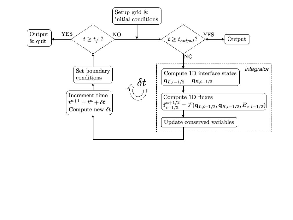
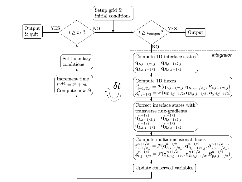

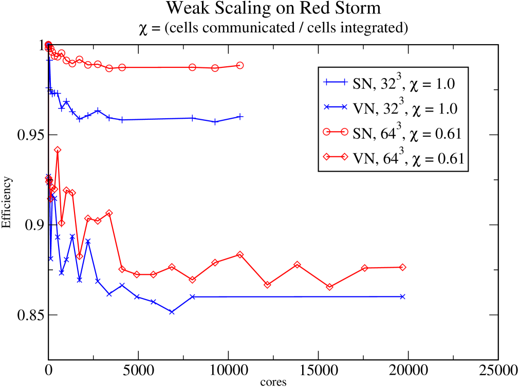


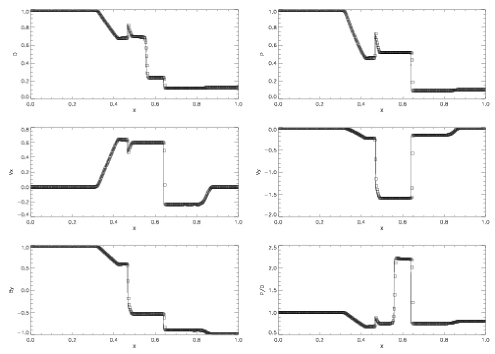
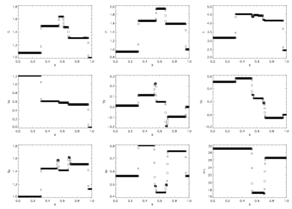
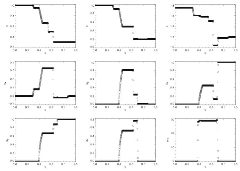


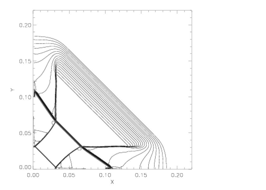
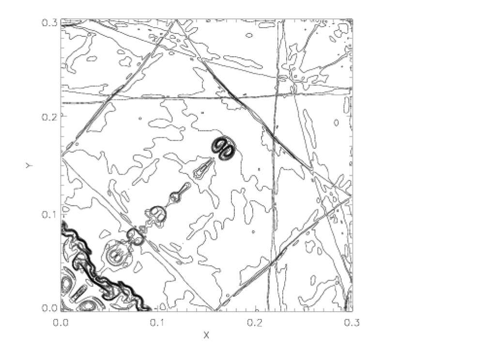

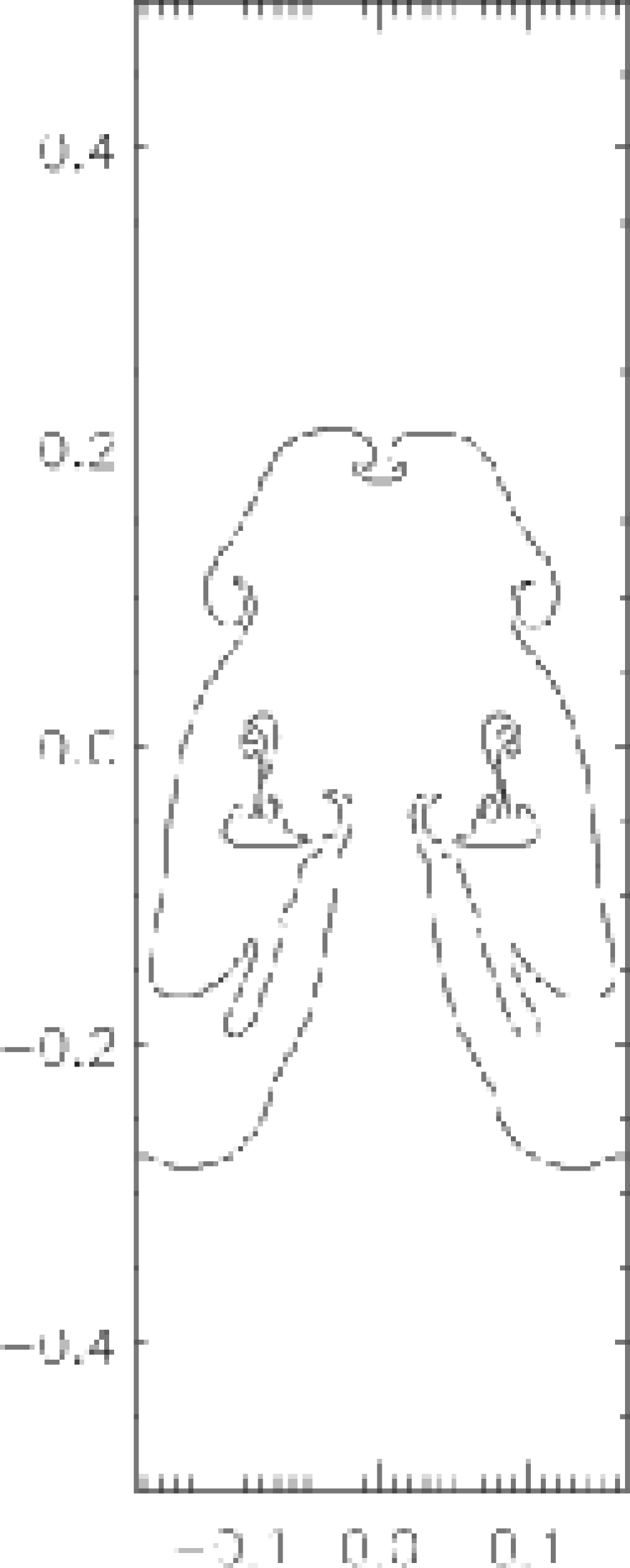


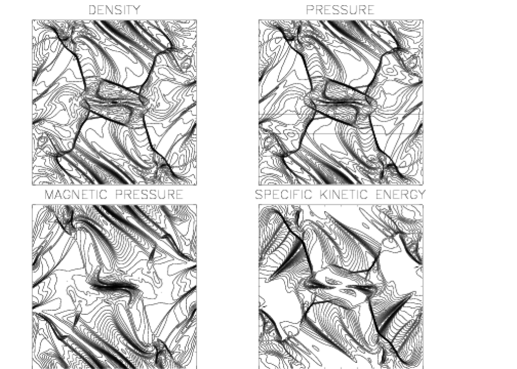

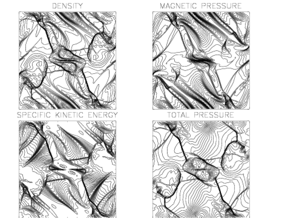
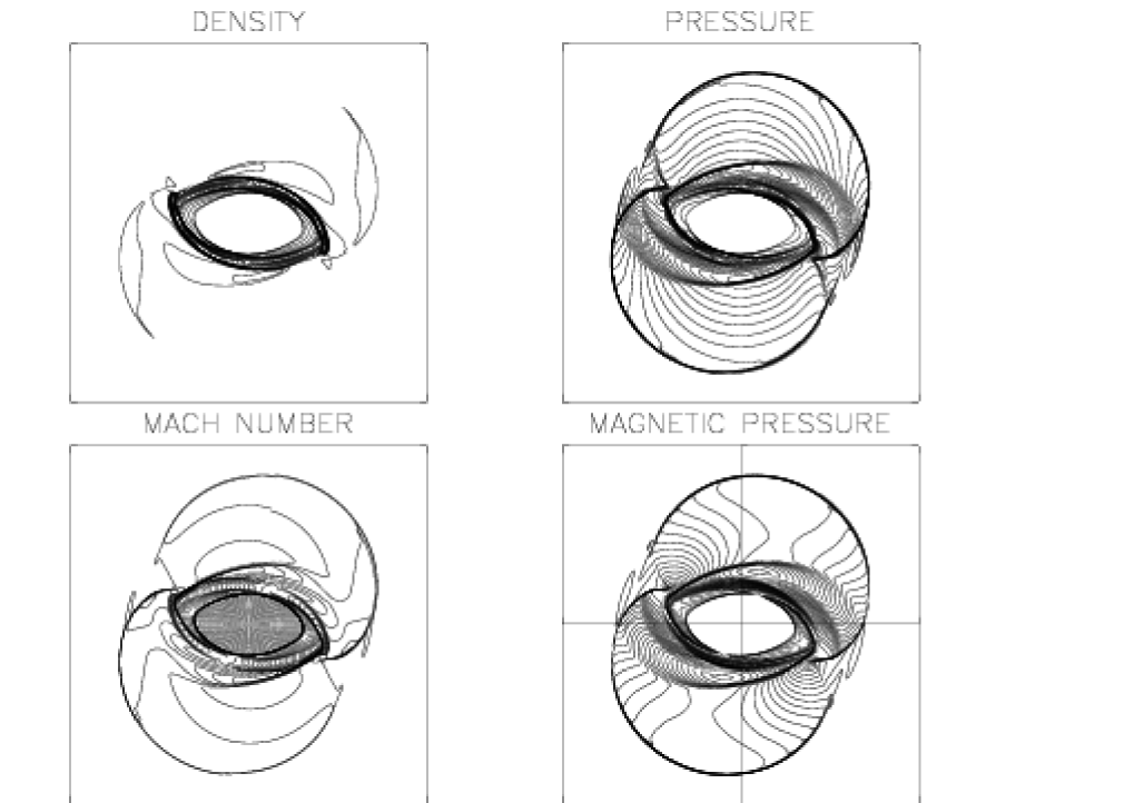

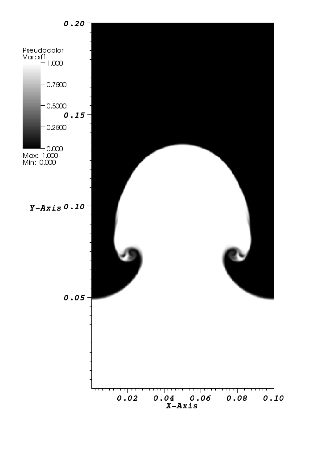
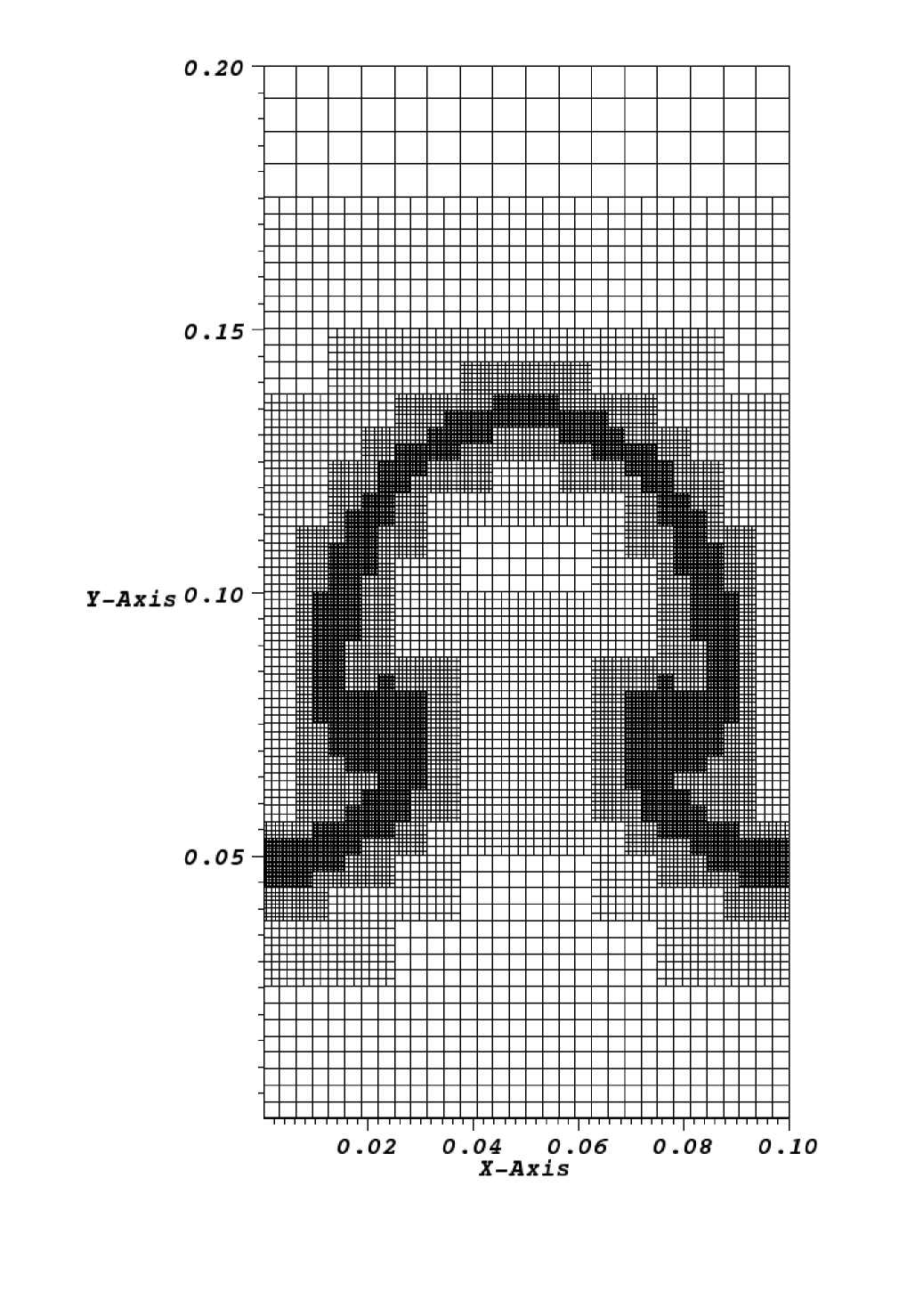
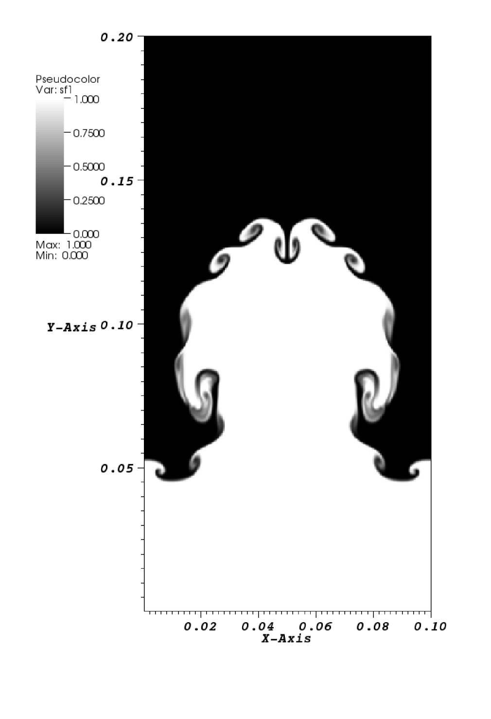
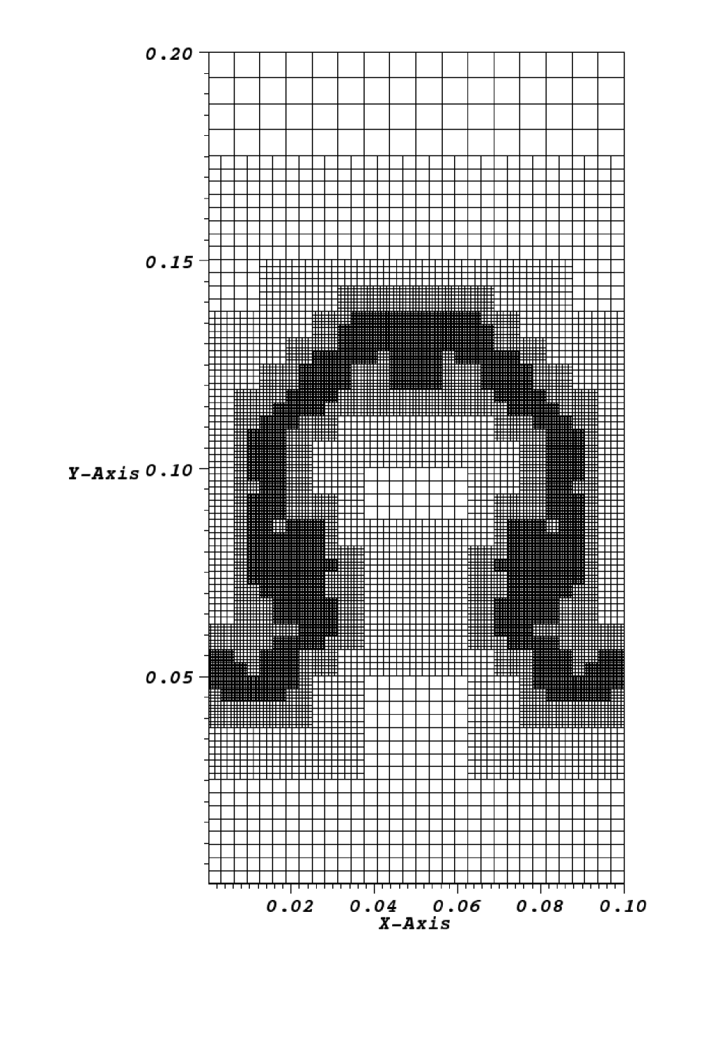
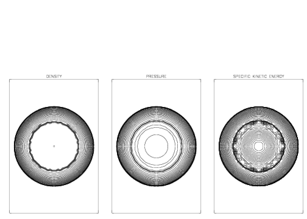
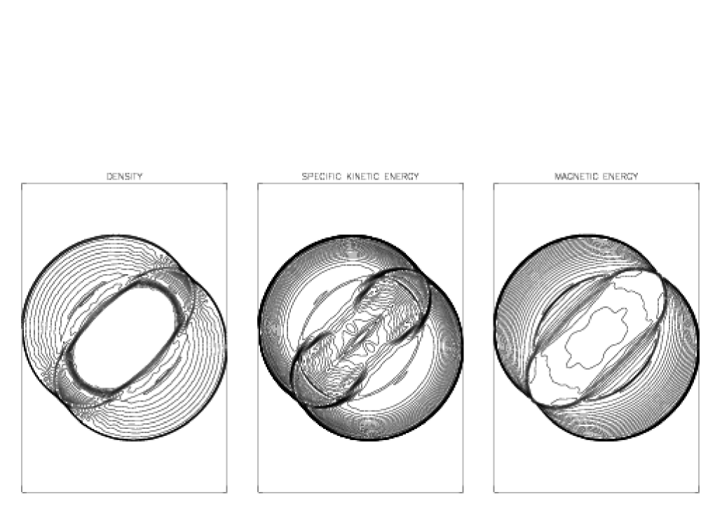
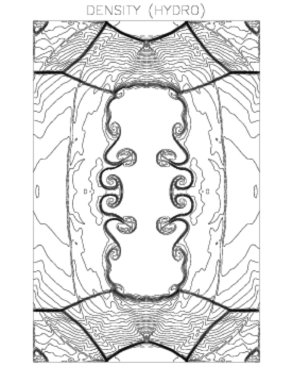
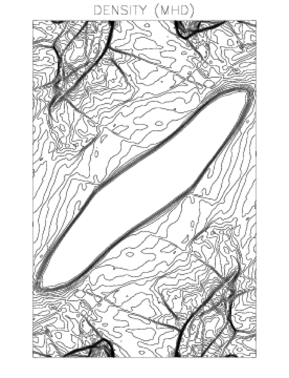
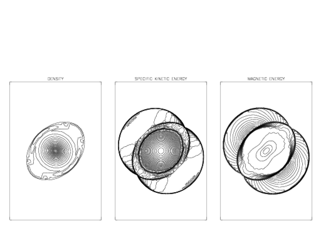
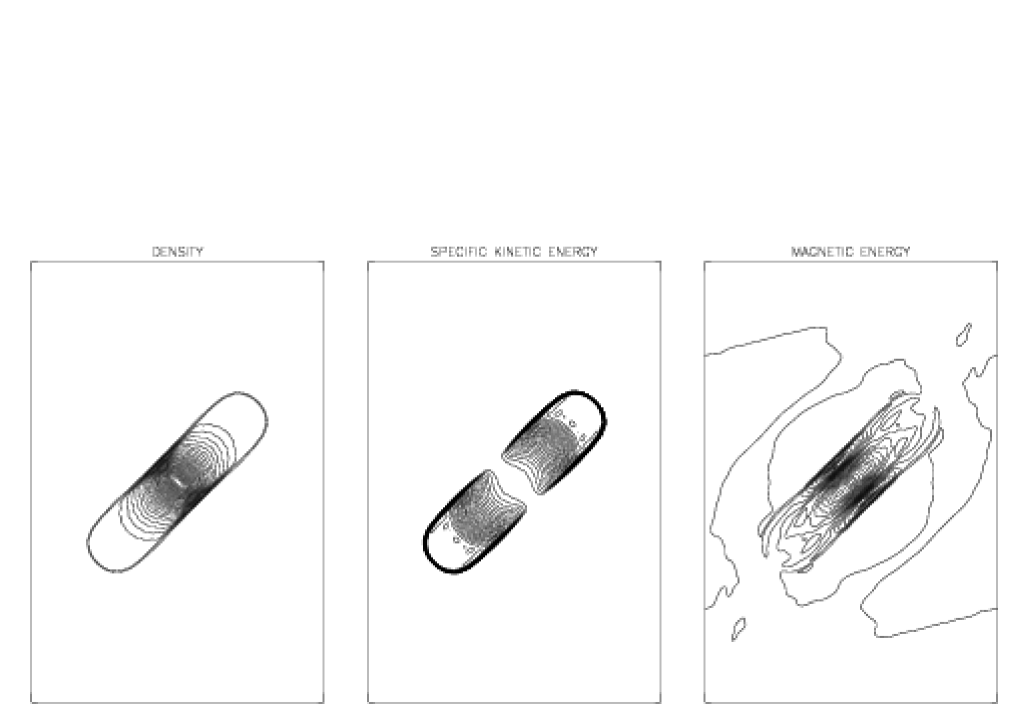
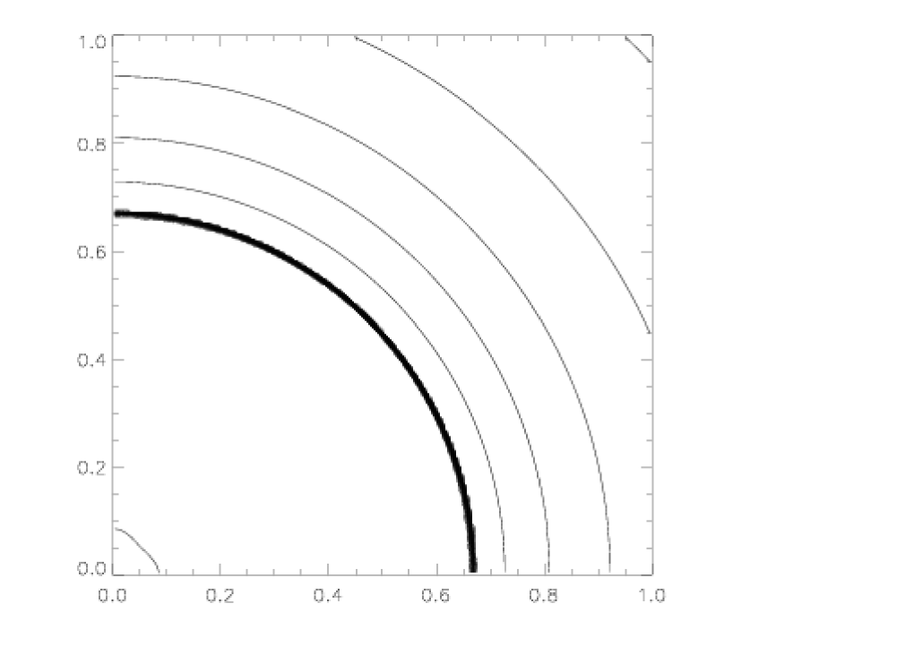
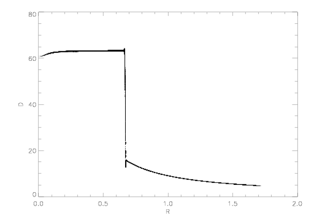


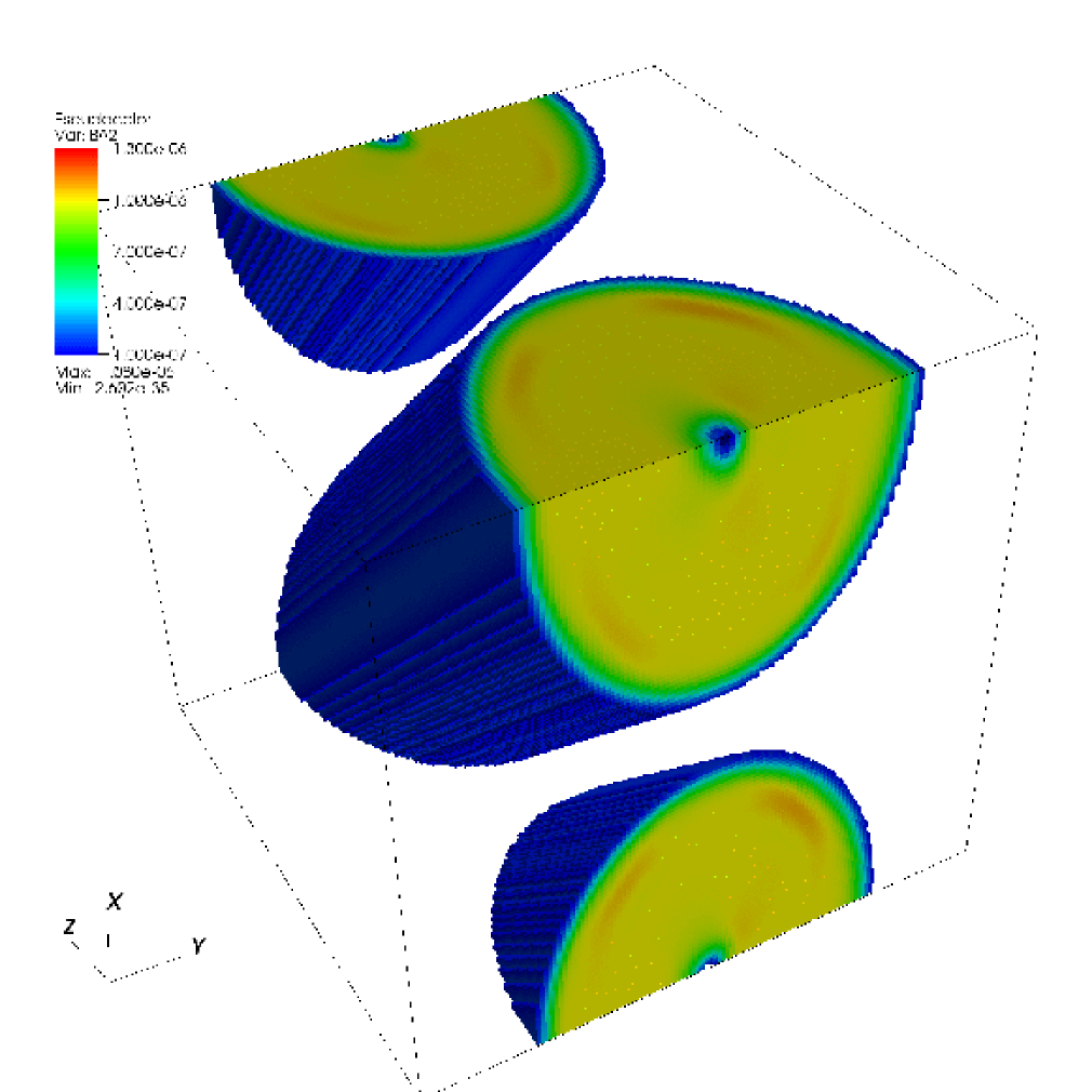
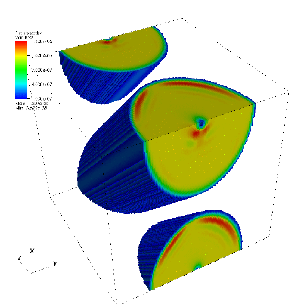
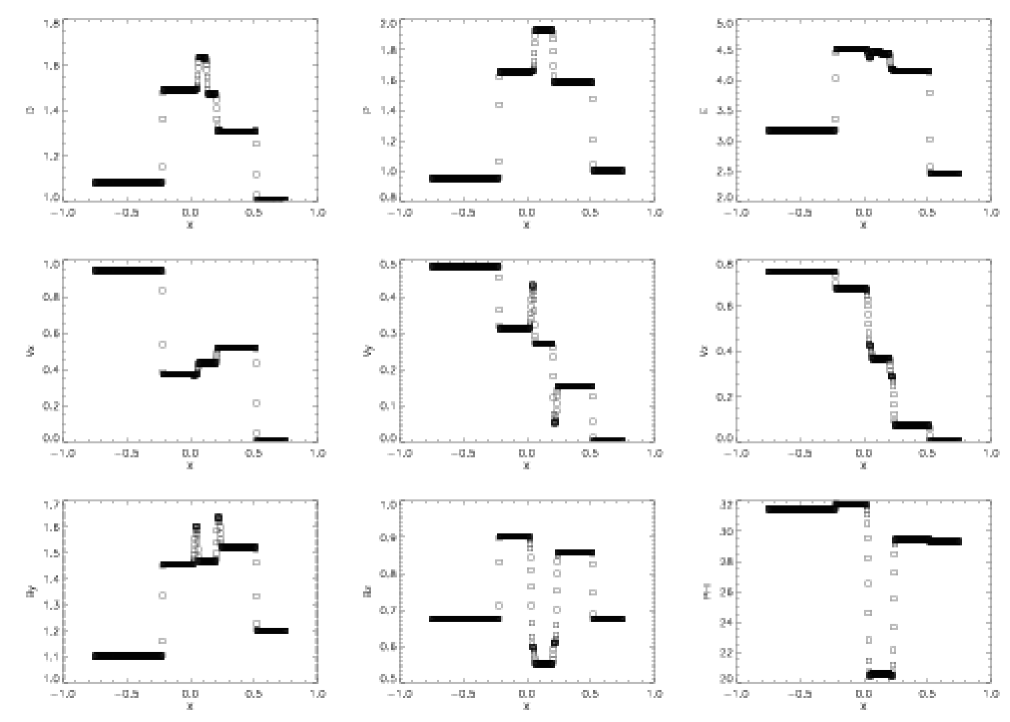
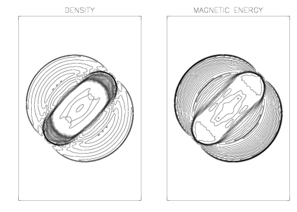
Appendix A Eigensystems in the Primitive Variables
This appendix gives explicit forms for the eigenvalues and eigenvectors of the matrix resulting from linearizing the dynamical equations as , where is a vector composed of the primitive variables in 1D. These eigensystems are needed to convert between the primitive and the characteristic variables in the reconstruction algorithms described in §4.2.
A.1 Adiabatic Hydrodynamics
For adiabatic hydrodynamics, , and the matrix is
| (A1) |
where ( is the adiabatic sound speed). The five eigenvalues of this matrix in ascending order are
| (A2) |
The corresponding right-eigenvectors are the columns of the matrix
| (A3) |
while the left-eigenvectors are the rows of the matrix
| (A4) |
A.2 Isothermal Hydrodynamics
For isothermal hydrodynamics, , and the matrix is
| (A5) |
where is the isothermal sound speed. The four eigenvalues of this matrix in ascending order are
| (A6) |
The corresponding right-eigenvectors are the columns of the matrix given in equation (A3), with the second column and fifth row dropped. The left-eigenvectors are the rows of the matrix
| (A7) |
A.3 Adiabatic Magnetohydrodynamics
For adiabatic MHD, , where , and the matrix is
| (A8) |
where . The seven eigenvalues of this matrix in ascending order are
| (A9) |
where the fast- and slow-magnetosonic wave speeds are given by
| (A10) |
(with given by the sign). The Alfvén speeds are given by
| (A11) |
The corresponding right-eigenvectors are the columns of the matrix
| (A12) |
where , and
| (A13) |
| (A14) |
| (A15) |
| (A16) |
| (A17) |
In the degenerate case where , so that , then equation (A16) becomes and . The left-eigenvectors are the rows of the matrix
| (A18) |
where
| (A19) |
are normalization factors for the eigenvectors corresponding to the fast- and slow-magnetosonic waves respectively.
A.4 Isothermal Magnetohydrodynamics
For isothermal MHD, , where , and the matrix is
| (A20) |
The six eigenvalues of this matrix in ascending order are
| (A21) |
where the fast and slow-magnetosonic wave speeds are given by equation (A10) (with replaced by the isothermal sound speed here and throughout), and the Alfvén speeds are given by equation (A11). The corresponding right-eigenvectors are the columns of the matrix given in equation (A10), with the fifth row and fourth column dropped. The left-eigenvectors are the rows of the matrix
| (A22) |
where
| (A23) |
are normalization factors for the eigenvectors corresponding to the fast- and slow-magnetosonic waves respectively.
Appendix B Eigensystems in the Conserved Variables
This appendix gives explicit forms for the eigenvalues and eigenvectors of the matrix resulting from linearizing the dynamical equations as , where is a vector composed of the conserved variables. These eigensystems are needed to construct the fluxes of the conserved quantities using Roe’s method (see §4.3.2).
B.1 Adiabatic Hydrodynamics
For adiabatic hydrodynamics, , and the matrix is
| (B1) |
where the enthalpy , , and . The five eigenvalues of this matrix in ascending order are
| (B2) |
where ( is the adiabatic sound speed). The corresponding right-eigenvectors are the columns of the matrix
| (B3) |
The left-eigenvectors are the rows of the matrix
| (B4) |
where . These are identical to those given by Roe (1981), except the second and third eigenvectors (corresponding to the transport of shear motion) have been rescaled to avoid singularities.
B.2 Isothermal Hydrodynamics
For isothermal hydrodynamics, , and the matrix is
| (B5) |
where is the isothermal sound speed. The four eigenvalues of this matrix in ascending order are
| (B6) |
The corresponding right-eigenvectors are the columns of the matrix given in equation (B3) with the fifth row and fourth column dropped, and replaced by throughout. The left-eigenvectors are the rows of the matrix
| (B7) |
B.3 Adiabatic Magnetohydrodynamics
For adiabatic MHD, , where , and the matrix is
| (B8) |
where , and
| (B9) |
| (B10) |
| (B11) |
| (B12) |
| (B13) |
| (B14) |
| (B15) |
| (B16) |
In these equations , , , and . The factors and are introduced by the averaging scheme defined by equation (56); thus the matrix and its eigenvectors depend explicitly on our choice of the Roe averaging scheme. The seven eigenvalues of this matrix in ascending order are
| (B17) |
where the fast and slow-magnetosonic wave speeds are given by
| (B18) |
(with given by the sign), and
| (B19) |
| (B20) |
The corresponding right-eigenvectors are the columns of the matrix
| (B21) |
where the and are given by equation (A13) to (A17) (with replaced by ), , and
| (B22) |
| (B23) |
| (B24) |
| (B25) |
| (B26) |
| (B27) |
where . In these equations
| (B28) |
The left-eigenvectors are the rows of the matrix
| (B29) |
where a symbol over the quantity denotes normalization via or . In addition,
| (B30) |
and
| (B31) |
| (B32) |
| (B33) |
| (B34) |
| (B35) |
| (B36) |
B.4 Isothermal Magnetohydrodynamics
For isothermal MHD, , where , and the matrix is
| (B37) |
where is the isothermal sound speed, and and are given by equations (B15) and (B16). The six eigenvalues of this matrix in ascending order are
| (B38) |
where the fast- and slow-magnetosonic wave speeds are given by
| (B39) |
(with given by the sign), where , and the Alfvén speeds are
| (B40) |
The corresponding right-eigenvectors are the columns of the matrix given by equation (B21) with the fifth row and fourth column dropped, and replaced by in the definitions given in equations (A15)-(A16). The left-eigenvectors are the rows of the matrix
| (B41) |
where , and are given by equations (A13)-(A15) (with replaced by ), are given by equation (A17), are given by equation (B30), and
| (B42) |
| (B43) |
| (B44) |
| (B45) |
In these equations, a symbol over the quantity denotes normalization via and .
Appendix C The H-correction: Fixing the Carbuncle Problem
For strong, planar shocks in multidimensions propagating along a grid direction, higher-order Godunov methods can be subject to a numerical instability (Quirk 1994) that grows into large amplitude perturbations of the shock front at the grid scale. This “carbuncle” instability can easily be demonstrated with a simple 2D test: a uniform high Mach number flow in the -direction is initialized everywhere in the domain, with inflow boundary conditions on the right boundary, and reflecting everywhere else. If zone-to-zone perturbations in the density with small amplitude () are added, the reflected shock will develop the carbuncle instability as it propagates to the left across the grid. Radiative cooling in the postshock gas can amplify the effect (Sutherland et al. 2003).
The source of the instability is the use of 1D Riemann solvers to compute fluxes in a multidimensional flow. When a planar shock is grid aligned, there is too little dissipation added to the fluxes in directions perpendicular to the shock front. Thus, small amplitude perturbations in the transverse direction grow, rather than being damped. The solution is to identify grid-aligned shocks and add extra dissipation to the transverse fluxes (e.g. Sutherland et al. 2003). In Athena, we use one form of the “H-correction” technique described in Sanders et al. (1998) to identify shocks and to add the appropriate dissipation.
The H-correction is most easily described when used in combination with the Roe fluxes. Consider the calculation of the flux at the interface located at in 2D. When the H-correction is used the absolute value of the eigenvalues in the Roe flux formula (equation 57) are replaced with , where for each component
| (C1) |
Note the max is taken over each independently in a pairwise fashion with , rather than over all eigenvalues at once. Here, comes from a 2D average using a five-point stencil in the shape of the letter ‘H’, that is
| (C2) |
where , is the component of the velocity normal to the interface, and is the fast magnetosonic speed (for MHD) in the direction normal to the interface. This correction is only added to the final multidimensional fluxes (computed in step 6 in 2D, and step 7 in 3D). It only becomes important in shocks, and for grid-aligned shocks it results in the dissipation in the transverse directions being comparable to that added in the direction of shock propagation. In 3D the H-correction generalizes to a 9-point average (one ‘H’ in each orthogonal plane). We find the HLL-type fluxes are less susceptible to the carbuncle instability, but are still affected by it in some circumstances. The H-correction can be added to HLL-type solvers by making the appropriate modification to the wavespeeds and defined in equations 53 and 54.
Use of the H-correction is only required for flows with strong, grid-aligned shocks (for most applications with Athena it is not needed). The results of the Noh strong shock test described in §8.5 show the H-correction is extremely effective at eliminating the carbuncle instability. In fact a variety of forms for the correction were proposed by Sanders et al. (see their equation 9). Tests using planar shocks in 2D subject to the carbuncle instability showed little difference between the formulations suggested by Sanders et al., thus we have chosen to adopt only the version described above.