Weak Lensing of the Primary CMB Bispectrum

Asantha Cooray, Devdeep Sarkar, and Paolo Serra Center for Cosmology, Department of Physics and Astronomy, University of California, Irvine, CA 92697
Abstract

The cosmic microwave background (CMB) bispectrum is a well-known probe of the non-Gaussianity of primordial perturbations. Just as the intervening large-scale structure modifies the CMB angular power spectrum through weak gravitational lensing, the CMB primary bispectrum generated at the last scattering surface is also modified by lensing. We discuss the lensing modification to the CMB bispectrum and show that lensing leads to an overall decrease in the amplitude of the primary bispectrum at multipoles of interest between 100 and 2000 through additional smoothing introduced by lensing. Since weak lensing is not accounted for in current estimators of the primordial non-Gaussianity parameter, the existing measurements of fNLsubscript𝑓NLf_{\rm NL} of the local model with WMAP out to lmax750similar-tosubscript𝑙max750l_{\rm max}\sim 750 is biased low by about 6%. For a high resolution experiment such as Planck, the lensing modification to the bispectrum must be properly included when attempting to estimate the primordial non-Gaussianity or the bias will be at the level of 30%. For Planck, weak lensing increases the minimum detectable value for the non-Gaussianity parameter of the local type fNLsubscript𝑓NLf_{\rm NL} to 7 from the previous estimate of about 5 without lensing. The minimum detectable value of fNLsubscript𝑓NLf_{\rm NL} for a cosmic variance limited experiment is also increased from less than 3 to similar-to\sim 5.

pacs:
98.70.Vc,98.65.Dx,95.85.Sz,98.80.Cq,98.80.Es

I Introduction

The weak lensing of cosmic microwave background (CMB) anisotropy angular power spectrum is now well understood in the literature lensing ; Lewis . The modifications result in a smoothing of the acoustic peak structure at large angular scales and an increase in power below a few arcminute angular scales corresponding to the the damping tail of CMB anisotropies Hu00 .

The angular power spectrum of the lensing potential out to the last scattering surface can be established with quadratic estimators that probe lensing non-Gaussianity at the 4-point level of a CMB map HuOka02 . Such a reconstruction of the lensing potential is helpful for CMB B-mode studies of polarization KamKosSte97 , especially in the context of searching for the signature of the primordial tensor modes KesCooKam02 . This is due to the fact that in addition to inflationary gravitational waves, the B-modes of CMB polarization also contains a signal generated by lensing of scalar E-modes with a peak in power at a few arcminute angular scales Zaldarriaga:1998ar . The lensing reconstruction has now been applied to the existing Wilkinson Microwave Anisotropy Probe (WMAP) data leading to a similar-to\sim 2σ𝜎\sigma to 3σ𝜎\sigma detection of gravitational lensing in the CMB through a correlation between the reconstructed lensing potential and tracers of the large-scale structure such as radio galaxies Smith ; Hirata .

In parallel with the progress on lensing studies with the CMB, the search for primordial non-Gaussianity using the CMB bispectrum with constraints on the non-Gaussianity parameter fNLsubscript𝑓NLf_{\rm NL} is now an active topic in cosmology Komatsu ; Lig ; Komatsu4 . The 5-year WMAP data is consistent with 9<fNL<1119subscript𝑓NL111-9<f_{\rm NL}<111 at the 95% confidence level for the local model Komatsu5yr , though a non-zero detection of primordial non-Gaussianity at the same 95% confidence level with 26.9<fNL<146.726.9subscript𝑓NL146.726.9<f_{\rm NL}<146.7 is claimed elsewhere using the WMAP 3-year data Yadav . This result, if correct, has significant cosmological implications since the expected value under standard inflationary models is fNL1less-than-or-similar-tosubscript𝑓NL1f_{\rm NL}\lesssim 1 Salopek ; Falk ; Gangui ; Pyne ; Acquaviva ; Maldacena ; Bartolo , though alternative models of inflation, such as the ekpyrotic cosmology Buchbinder ; Lehners , generally predict a large primordial non-Gaussianity with fNLsubscript𝑓NLf_{\rm NL} at few tens.

Just as the CMB power spectrum is modified by lensing from potential fluctuations of the intervening large-scale structure lensing , the CMB bispectrum will also be modified by gravitational lensing. The correlation between the projected lensing potential and CMB secondary effects, such as the integrated Sachs-Wolfe (ISW) effect or the Sunyaev-Zel’dovich (SZ) effect, leads to a non-Gaussian signal at the three point level Goldberg ; Cooray . These secondary non-Gaussianities are expected even if the primordial perturbations are Gaussian and impact existing primordial non-Gaussianity parameter measurements by introducing a small, but unavoidable, bias Smith2 ; Serra ; BabichPier .

Beyond secondary non-Gaussianities, weak lensing by the intervening large-scale structure maps the intrinsically non-Gaussian CMB sky to a different anisotropy pattern when observed today. Thus the bispectrum one reconstructs with a CMB map, assuming it to be of the expected form at the last-scattering surface due to primordial non-Gaussian perturbations, will result in a biased estimate of the primordial non-Gaussianity parameter. The existing estimator can be modified to account for lensing modifications and to obtain a bias-free estimate of the non-Gaussianity, but at the expense of factorizability that has allowed fast computation of the bispectrum in existing analyses Komatsu2 . Since lensing modifies the anisotropy pattern by smoothing the fluctuations, a change in the minimum detectable non-Gaussianity parameter fNLsubscript𝑓NLf_{\rm NL} for a given experiment is expected to be different from the existing values in the literature Komatsu .

In this paper, we present a general derivation of the lensed CMB primary bispectrum and quantify above statements on the changes imposed by lensing for the detection of primordial non-Gaussianity. We find that the non-Gaussianity parameter measured with WMAP, ignoring lensing, will result in an estimate of fNLsubscript𝑓NLf_{\rm NL} for the local model that is biased low by about 6%, when measurements are extended out to lmax750similar-tosubscript𝑙max750l_{\rm max}\sim 750. Furthermore, with lensing, the minimum detectable level of fNLsubscript𝑓NLf_{\rm NL} with Planck is increased by roughly 40% from less than 5 to about 7 and the cosmic variance limit of fNLsubscript𝑓NLf_{\rm NL} is increased from 3 to 5.

This paper is organized as follows: we first discuss the CMB primary bispectrum of the local type in Section II. Some basic ingredients related to the lensing calculation is presented in Section III. We derive the lensing effect on the bispectrum, under both flat-sky and all-sky formulations, in Section IV. We discuss our results and conclude with a summary in Section V. In illustrating our results we make use of the standard flat ΛΛ\LambdaCDM cosmological model consistent with WMAP with Ωb=0.042subscriptΩ𝑏0.042\Omega_{b}=0.042, Ωc=0.238subscriptΩ𝑐0.238\Omega_{c}=0.238, h=0.7320.732h=0.732, ns=0.958subscript𝑛𝑠0.958n_{s}=0.958 and τ=0.089𝜏0.089\tau=0.089.

II CMB Primary Bispectrum

The CMB temperature perturbation on the sky, Θ(𝐧^)=ΔT(𝐧^)/TΘ^𝐧Δ𝑇^𝐧𝑇{\Theta}({\bf\hat{n}})=\Delta T({\bf\hat{n}})/T, is decomposed into its multipole moments

Θ(𝐧^)=lmΘlmYlm(𝐧^).Θ^𝐧subscript𝑙𝑚subscriptΘ𝑙𝑚superscriptsubscript𝑌𝑙𝑚^𝐧{\Theta}({\bf\hat{n}})=\sum_{lm}{\Theta}_{lm}Y_{l}^{m}({\bf\hat{n}})\,. (1)

The angular power spectrum and bispectrum of CMB anisotropies are defined in the usual way, respectively, as

ΘlmΘlmdelimited-⟨⟩subscriptΘ𝑙𝑚subscriptΘsuperscript𝑙superscript𝑚\displaystyle\langle{\Theta}_{lm}{\Theta}_{l^{\prime}m^{\prime}}\rangle =\displaystyle= δl,lδm,mClΘΘ,subscript𝛿𝑙superscript𝑙subscript𝛿𝑚superscript𝑚superscriptsubscript𝐶𝑙ΘΘ\displaystyle\delta_{l,l^{\prime}}\delta_{m,m^{\prime}}C_{l}^{{\Theta}{\Theta}}\,,
Θl1m1Θl2m2Θl3m3delimited-⟨⟩subscriptΘsubscript𝑙1subscript𝑚1subscriptΘsubscript𝑙2subscript𝑚2subscriptΘsubscript𝑙3subscript𝑚3\displaystyle\langle{\Theta}_{l_{1}m_{1}}{\Theta}_{l_{2}m_{2}}{\Theta}_{l_{3}m_{3}}\rangle =\displaystyle= (l1l2l3m1m2m3)Bl1l2l3,subscript𝑙1subscript𝑙2subscript𝑙3subscript𝑚1subscript𝑚2subscript𝑚3subscript𝐵subscript𝑙1subscript𝑙2subscript𝑙3\displaystyle\left(\begin{array}[]{ccc}\!l_{1}\!&l_{2}\!&l_{3}\!\\ \!m_{1}\!&m_{2}\!&m_{3}\!\end{array}\right)B_{l_{1}l_{2}l_{3}}\,, (4)

where, for the bispectrum, we have introduced the Wigner-3j𝑗j symbol (see the Appendix of Ref. Cooray for some useful properties of this symbol).

The CMB bispectrum is generated by a coupling of the local-type with a quadratic correction to the Newtonian curvature such that

Φ(𝐱)=ΦL(𝐱)+fNL[ΦL2(𝐱)ΦL2(𝐱)]Φ𝐱subscriptΦ𝐿𝐱subscript𝑓NLdelimited-[]subscriptsuperscriptΦ2𝐿𝐱delimited-⟨⟩subscriptsuperscriptΦ2𝐿𝐱\Phi({\bf x})=\Phi_{L}({\bf x})+{f_{\rm NL}}\left[\Phi^{2}_{L}({\bf x})-\langle\Phi^{2}_{L}({\bf x})\rangle\right]\, (5)

where ΦL(𝐱)subscriptΦ𝐿𝐱\Phi_{L}({\bf x}) is the linear and Gaussian perturbation and fNLsubscript𝑓NL{f_{\rm NL}} in the non-Gaussianity parameter, which is taken to be scale independent Komatsu .

In Fourier space, we can decompose equation (5) as

Φ(𝐤)=ΦL(𝐤)+fNLΦNL(𝐤),Φ𝐤subscriptΦ𝐿𝐤subscript𝑓NLsubscriptΦNL𝐤\Phi({\bf k})=\Phi_{L}({\bf k})+f_{\rm NL}\Phi_{\rm NL}({\bf k})\,, (6)

with

ΦNL(𝐤)subscriptΦNL𝐤\displaystyle\Phi_{\rm NL}({\bf k}) =\displaystyle= d3𝐤1(2π)3ΦL(𝐤+𝐤1)ΦL(𝐤1)superscript𝑑3subscript𝐤1superscript2𝜋3subscriptΦ𝐿𝐤subscript𝐤1superscriptsubscriptΦ𝐿subscript𝐤1\displaystyle\int\frac{d^{3}{{\bf k}_{1}}}{(2\pi)^{3}}\Phi_{L}({\bf k}+{\bf k}_{1})\Phi_{L}^{*}({\bf k}_{1}) (7)
(2π)3δ(𝐤)d3𝐤1(2π)3PΦ(k1),superscript2𝜋3𝛿𝐤superscript𝑑3subscript𝐤1superscript2𝜋3subscript𝑃Φsubscript𝑘1\displaystyle-(2\pi)^{3}\delta({\bf k})\int\frac{d^{3}{{\bf k}_{1}}}{(2\pi)^{3}}P_{\Phi}(k_{1})\,,

where PΦ(k)subscript𝑃Φ𝑘P_{\Phi}(k) is the linear power spectrum, defined as

Φ(𝐤)Φ(𝐤)=(2π)3δ(𝐤+𝐤)PΦ(k).delimited-⟨⟩Φ𝐤Φsuperscript𝐤superscript2𝜋3𝛿𝐤superscript𝐤subscript𝑃Φ𝑘\langle\Phi({\bf k})\Phi({\bf k}^{\prime})\rangle=(2\pi)^{3}\delta({\bf k}+{\bf k}^{\prime})P_{\Phi}(k)\,. (8)

The multipole moments of the anisotropy can be written as

Θlm=4π(i)ld3𝐤(2π)3Φ(𝐤)gTl(k)Ylm(𝐤^),subscriptΘ𝑙𝑚4𝜋superscript𝑖𝑙superscript𝑑3𝐤superscript2𝜋3Φ𝐤subscript𝑔𝑇𝑙𝑘superscriptsubscript𝑌𝑙𝑚^𝐤{\Theta}_{lm}=4\pi(-i)^{l}\int\frac{d^{3}{\mathbf{k}}}{(2\pi)^{3}}\Phi({\mathbf{k}})g_{Tl}(k)Y_{lm}^{*}(\hat{\mathbf{k}}), (9)

where Φ(𝐤)Φ𝐤\Phi({\mathbf{k}}) from above is the primordial curvature perturbation in the Fourier space, and gTl(k)subscript𝑔𝑇𝑙𝑘g_{Tl}(k) is the radiation transfer function. With ΦL(𝐤)subscriptΦ𝐿𝐤\Phi_{L}({\bf k}) and ΦNLsubscriptΦNL\Phi_{\rm NL}, the moments can be separated into two components with Θlm=ΘlmL+ΘlmNLsubscriptΘ𝑙𝑚superscriptsubscriptΘ𝑙𝑚𝐿superscriptsubscriptΘ𝑙𝑚𝑁𝐿{\Theta}_{lm}={\Theta}_{lm}^{L}+{\Theta}_{lm}^{NL}.

The CMB angular power spectrum can be defined using the transfer function and the power spectrum of dominant linear fluctuations as

ClΘ=2π0k2𝑑kPΦ(k)gTl2(k).superscriptsubscript𝐶𝑙Θ2𝜋superscriptsubscript0superscript𝑘2differential-d𝑘subscript𝑃Φ𝑘subscriptsuperscript𝑔2𝑇𝑙𝑘C_{l}^{\Theta}=\frac{2}{\pi}\int_{0}^{\infty}k^{2}dkP_{\Phi}(k)g^{2}_{Tl}(k)\,. (10)

Using the definition of the angular bispectrum (equation 4), the primordial temperature anisotropy bispectrum can be written as

Bl1l2l3=m1m2m3(l1l2l3m1m2m3)[Θl1m1LΘl2m2LΘl3m3NL\displaystyle B_{l_{1}l_{2}l_{3}}=\sum_{m_{1}m_{2}m_{3}}\left(\begin{array}[]{ccc}l_{1}&l_{2}&l_{3}\\ m_{1}&m_{2}&m_{3}\end{array}\right)\bigg{[}\langle{\Theta}_{l_{1}m_{1}}^{L}{\Theta}_{l_{2}m_{2}}^{L}{\Theta}_{l_{3}m_{3}}^{NL}\rangle (13)
+Θl1m1LΘl2m2NLΘl3m3L+Θl1m1NLΘl2m2LΘl3m3L],\displaystyle+\langle{\Theta}_{l_{1}m_{1}}^{L}{\Theta}_{l_{2}m_{2}}^{NL}{\Theta}_{l_{3}m_{3}}^{L}\rangle+\langle{\Theta}_{l_{1}m_{1}}^{NL}{\Theta}_{l_{2}m_{2}}^{L}{\Theta}_{l_{3}m_{3}}^{L}\rangle\bigg{]}\,, (14)

which can be simplified to Komatsu

Bl1l2l3subscript𝐵subscript𝑙1subscript𝑙2subscript𝑙3\displaystyle B_{l_{1}l_{2}l_{3}} =\displaystyle= 2𝒢l1l2l30r2𝑑rbl1L(r)bl2L(r)bl3NL(r)2subscript𝒢subscript𝑙1subscript𝑙2subscript𝑙3superscriptsubscript0superscript𝑟2differential-d𝑟subscriptsuperscript𝑏𝐿subscript𝑙1𝑟subscriptsuperscript𝑏𝐿subscript𝑙2𝑟subscriptsuperscript𝑏𝑁𝐿subscript𝑙3𝑟\displaystyle 2{\cal G}_{l_{1}l_{2}l_{3}}\int_{0}^{\infty}r^{2}drb^{L}_{l_{1}}(r)b^{L}_{l_{2}}(r)b^{NL}_{l_{3}}(r)
+bl1L(r)bl2NL(r)bl3L(r)+bl1NL(r)bl2L(r)bl3L(r),subscriptsuperscript𝑏𝐿subscript𝑙1𝑟subscriptsuperscript𝑏𝑁𝐿subscript𝑙2𝑟subscriptsuperscript𝑏𝐿subscript𝑙3𝑟subscriptsuperscript𝑏𝑁𝐿subscript𝑙1𝑟subscriptsuperscript𝑏𝐿subscript𝑙2𝑟subscriptsuperscript𝑏𝐿subscript𝑙3𝑟\displaystyle+b^{L}_{l_{1}}(r)b^{NL}_{l_{2}}(r)b^{L}_{l_{3}}(r)+b^{NL}_{l_{1}}(r)b^{L}_{l_{2}}(r)b^{L}_{l_{3}}(r),

where

blL(r)subscriptsuperscript𝑏𝐿𝑙𝑟\displaystyle b^{L}_{l}(r) =\displaystyle= 2π0k2𝑑kPΦ(k)gTl(k)jl(kr),2𝜋superscriptsubscript0superscript𝑘2differential-d𝑘subscript𝑃Φ𝑘subscript𝑔𝑇𝑙𝑘subscript𝑗𝑙𝑘𝑟\displaystyle\frac{2}{\pi}\int_{0}^{\infty}k^{2}dkP_{\Phi}(k)g_{Tl}(k)j_{l}(kr), (16)
blNL(r)subscriptsuperscript𝑏𝑁𝐿𝑙𝑟\displaystyle b^{NL}_{l}(r) =\displaystyle= fNL2π0k2𝑑kgTl(k)jl(kr),subscript𝑓NL2𝜋superscriptsubscript0superscript𝑘2differential-d𝑘subscript𝑔𝑇𝑙𝑘subscript𝑗𝑙𝑘𝑟\displaystyle{f_{\rm NL}}\frac{2}{\pi}\int_{0}^{\infty}k^{2}dkg_{Tl}(k)j_{l}(kr)\,, (17)

and

𝒢l1l2l3=(2l1+1)(2l2+1)(2l3+1)4π(l1l2l3000).subscript𝒢subscript𝑙1subscript𝑙2subscript𝑙32subscript𝑙112subscript𝑙212subscript𝑙314𝜋subscript𝑙1subscript𝑙2subscript𝑙3000{\cal G}_{l_{1}l_{2}l_{3}}=\sqrt{\frac{(2l_{1}+1)(2l_{2}+1)(2l_{3}+1)}{4\pi}}\left(\begin{array}[]{ccc}l_{1}&l_{2}&l_{3}\\ 0&0&0\end{array}\right)\,. (18)

When illustrating our results, we make use of a modified code of CMBFAST Seljak for the standard flat ΛΛ\LambdaCDM cosmological model to fully calculate radiation transfer functions when generating the CMB primary bispectrum.
Refer to caption
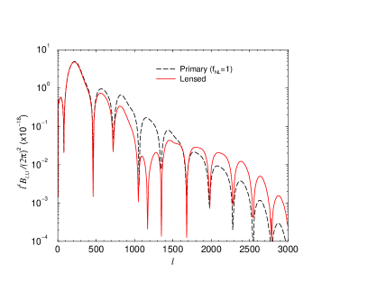
Figure 1: The CMB bispectrum for the equilateral case (l1=l2=l3=lsubscript𝑙1subscript𝑙2subscript𝑙3𝑙l_{1}=l_{2}=l_{3}=l) with (solid line) and without (dashed line) lensing. Here we plot l4Blllθ/(2π)2superscript𝑙4subscriptsuperscript𝐵𝜃𝑙𝑙𝑙superscript2𝜋2l^{4}B^{\theta}_{lll}/(2\pi)^{2} as a function of the multipole l𝑙l for one of the sides. We assume fNL=1subscript𝑓NL1f_{\rm NL}=1. The lensing effect can be described as a decrease in the amplitude of the bispectrum when l1700less-than-or-similar-to𝑙1700l\lesssim 1700 with an increase at higher multipoles.

III Weak Lensing Basics

The effects of weak lensing can be encapsulated, under the Born approximation, in the radial projection of the gravitational potential (ΦΦ\Phi), given as cosmicshearrefs

ϕ(𝐧^)italic-ϕ^𝐧\displaystyle\phi({\bf\hat{n}}) =\displaystyle= 20rs𝑑rdA(rsr)dA(rs)dA(r)Φ(𝐫(𝐧^),r),2superscriptsubscript0subscript𝑟𝑠differential-dsuperscript𝑟subscript𝑑𝐴subscript𝑟𝑠superscript𝑟subscript𝑑𝐴subscript𝑟𝑠subscript𝑑𝐴superscript𝑟Φ𝐫^𝐧superscript𝑟\displaystyle-2\int_{0}^{{r}_{s}}d{r}^{\prime}\frac{{d_{A}}({r}_{s}-{r}^{\prime})}{{d_{A}}({r}_{s}){d_{A}}({r}^{\prime})}\Phi(\mathbf{r}(\hat{{\bf n}}),{r}^{\prime})\,, (19)

where r(z)𝑟𝑧{r}(z) is the line-of-sight comoving distance (or look-back time) to a redshift z𝑧z from the observer with last scattering surface at rs=r(z=1100)subscript𝑟𝑠𝑟𝑧1100{r}_{s}={r}(z=1100), and dA(r)subscript𝑑𝐴𝑟{d_{A}}({r}) is the comoving angular diameter distance. In a spatially flat universe, dArsubscript𝑑𝐴𝑟{d_{A}}\rightarrow{r}. Here, we ignore the time-delay effect as it is small compared to the geometric lensing effect captured by equation (19) CooHutime .

The calculation related to the CMB bispectrum described below requires the angular power spectrum of lensing potential ϕitalic-ϕ\phi, which can be decomposed into the multiple moments as

ϕ(𝐧^)=lmϕlmYlm(𝐧^),italic-ϕ^𝐧subscript𝑙𝑚subscriptitalic-ϕ𝑙𝑚superscriptsubscript𝑌𝑙𝑚^𝐧\phi({\bf\hat{n}})=\sum_{lm}\phi_{lm}Y_{l}^{m}({\bf\hat{n}})\,, (20)

with the lensing power spectrum defined using ϕlmϕlm=δl,lδm,mClϕdelimited-⟨⟩subscriptitalic-ϕ𝑙𝑚subscriptitalic-ϕsuperscript𝑙superscript𝑚subscript𝛿𝑙superscript𝑙subscript𝛿𝑚superscript𝑚subscriptsuperscript𝐶italic-ϕ𝑙\langle\phi_{lm}\phi_{l^{\prime}m^{\prime}}\rangle=\delta_{l,l^{\prime}}\delta_{m,m^{\prime}}C^{\phi}_{l} to obtain Hu00

Clϕ=2πk2𝑑kPΦ(k)[Illen(k)]2,superscriptsubscript𝐶𝑙italic-ϕ2𝜋superscript𝑘2differential-d𝑘subscript𝑃Φ𝑘superscriptdelimited-[]superscriptsubscript𝐼𝑙len𝑘2C_{l}^{\phi}=\frac{2}{\pi}\int k^{2}dkP_{\Phi}(k)[I_{l}^{\rm len}(k)]^{2}\,, (21)

where

Illen(k)superscriptsubscript𝐼𝑙len𝑘\displaystyle I_{l}^{\rm len}(k) =\displaystyle= 𝑑rWlen(r)jl(kr),differential-d𝑟superscript𝑊len𝑟subscript𝑗𝑙𝑘𝑟\displaystyle\int d{r}\,W^{\rm len}({r})j_{l}(k{r})\,,
Wlen(r)superscript𝑊len𝑟\displaystyle W^{\rm len}({r}) =\displaystyle= 2F(r)dA(rsr)dA(r)dA(rs).2𝐹𝑟subscript𝑑𝐴subscript𝑟𝑠𝑟subscript𝑑𝐴𝑟subscript𝑑𝐴subscript𝑟𝑠\displaystyle-2F({r}){{d_{A}}({r}_{s}-{r})\over{d_{A}}({r}){d_{A}}({r}_{s})}\,. (22)

Here F(r)𝐹𝑟F({r}) describes the radial evolution of potential fluctuations. Modifications to the CMB anisotropies, generated at higher order in lensing potential fluctuations, are at the level of at most 5% relative to those due to the lensing potential angular power spectrum Cooray3 . The bispectrum of lensing potentials, due to the non-linear evolution of density perturbations, also modifies the CMB primary bispectrum, but these changes can also be ignored since the lensing potential bispectrum is at the order (Clϕ)2superscriptsuperscriptsubscript𝐶𝑙italic-ϕ2\left(C_{l}^{\phi}\right)^{2}, while changes we describe are first order in the angular power spectrum of the lensing potential. Using the Limber approximation, equation (21) can be further simplified, but we do not make use of this approximation in numerical calculations illustrated here since the flat-sky form of the potential power spectrum is known to bias lensing results of the power spectrum by about 10% at all multipoles Hu00 .

IV Lensing of the CMB Bispectrum

We first give a treatment of the lensing of the CMB bispectrum assuming a flat-sky approximation and discuss a derivation under the spherical sky later.
Refer to caption
Refer to caption
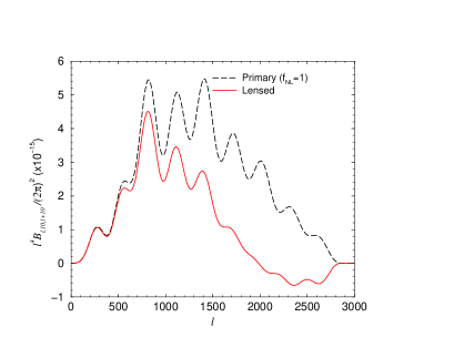
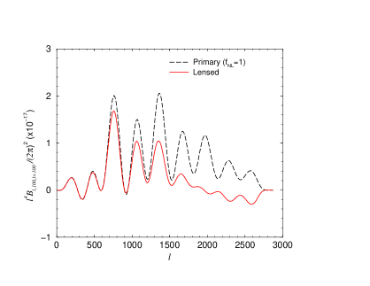
Figure 2: The squeezed configurations (l1l3l2similar-tosubscript𝑙1subscript𝑙3much-greater-thansubscript𝑙2l_{1}\sim l_{3}\gg l_{2}) of the CMB bispectrum with (solid line) and without (dashed line) lensing. The left panel is for l2=10subscript𝑙210l_{2}=10 and right panel is l2=100subscript𝑙2100l_{2}=100. We vary l=l1𝑙subscript𝑙1l=l_{1} with l3=l+l2subscript𝑙3𝑙subscript𝑙2l_{3}=l+l_{2} in both cases and plot l4Bl,l2,l+l2/(2π)2superscript𝑙4subscript𝐵𝑙subscript𝑙2𝑙subscript𝑙2superscript2𝜋2l^{4}B_{l,l_{2},l+l_{2}}/(2\pi)^{2} as a function of l𝑙l. Again, we take fNL=1subscript𝑓NL1f_{\rm NL}=1. In these configurations, the lensing effect can be described as an overall decrease in the amplitude of the bispectrum when l1200less-than-or-similar-to𝑙1200l\lesssim 1200. This suggests that lensing by the intervening large-scale structure leads to a less non-Gaussianity in the CMB map.

IV.1 Flat-sky Case

Weak lensing deflects the path of background photons resulting in a remapping of the observed anisotropy pattern on the sky. Following an approach similar to Hu00 , we write the lensed temperature anisotropy as

Θ~(𝐧^)~Θ^𝐧\displaystyle\tilde{\Theta}({\bf\hat{n}}) =\displaystyle= Θ[𝐧^+ϕ(𝐧^)]Θdelimited-[]^𝐧italic-ϕ^𝐧\displaystyle{\Theta}[{\bf\hat{n}}+\nabla\phi({\bf\hat{n}})] (23)
\displaystyle\approx Θ(𝐧^)+iϕ(𝐧^)iΘ(𝐧^)Θ^𝐧subscript𝑖italic-ϕ^𝐧superscript𝑖Θ^𝐧\displaystyle{\Theta}({\bf\hat{n}})+\nabla_{i}\phi({\bf\hat{n}})\nabla^{i}{\Theta}({\bf\hat{n}})
+12iϕ(𝐧^)jϕ(𝐧^)ijΘ(𝐧^)+12subscript𝑖italic-ϕ^𝐧subscript𝑗italic-ϕ^𝐧superscript𝑖superscript𝑗Θ^𝐧\displaystyle+{1\over 2}\nabla_{i}\phi({\bf\hat{n}})\nabla_{j}\phi({\bf\hat{n}})\nabla^{i}\nabla^{j}{\Theta}({\bf\hat{n}})+\ldots\;

Here, Θ(𝐧^)Θ^𝐧{\Theta}({\bf\hat{n}}) is the unlensed CMB temperature anisotropy, Θ~(𝐧^)~Θ^𝐧\tilde{\Theta}({\bf\hat{n}}) is the lensed anisotropy, and ϕ(𝐧^)italic-ϕ^𝐧\nabla\phi({\bf\hat{n}}) is the lensing deflection angle for the CMB photons.

Taking the Fourier transform, as appropriate for a flat-sky, we write the lensed temperature anisotropy in Fourier space as

Θ~(𝐥1)~Θsubscript𝐥1\displaystyle\tilde{\Theta}({{\bf l}_{1}}) =\displaystyle= 𝑑𝐧^Θ~(𝐧^)ei𝐥1𝐧^differential-d^𝐧~Θ^𝐧superscript𝑒𝑖subscript𝐥1^𝐧\displaystyle\int d{\bf\hat{n}}\,\tilde{\Theta}({\bf\hat{n}})e^{-i{{\bf l}_{1}}\cdot{\bf\hat{n}}} (24)
=\displaystyle= Θ(𝐥1)d2𝐥1(2π)2Θ(𝐥1)L(𝐥1,𝐥1),Θsubscript𝐥1superscript𝑑2superscriptsubscript𝐥1superscript2𝜋2Θsuperscriptsubscript𝐥1𝐿subscript𝐥1superscriptsubscript𝐥1\displaystyle{\Theta}({{\bf l}_{1}})-\int{d^{2}{\bf l}_{1}^{\prime}\over(2\pi)^{2}}{\Theta}({{\bf l}_{1}}^{\prime})L({{\bf l}_{1}},{{\bf l}_{1}}^{\prime})\,,

where

L(𝐥1,𝐥1)𝐿subscript𝐥1superscriptsubscript𝐥1\displaystyle L({{\bf l}_{1}},{{\bf l}_{1}}^{\prime}) \displaystyle\equiv ϕ(𝐥1𝐥1)(𝐥1𝐥1)𝐥1italic-ϕsubscript𝐥1superscriptsubscript𝐥1subscript𝐥1superscriptsubscript𝐥1superscriptsubscript𝐥1\displaystyle\phi({{\bf l}_{1}}-{{\bf l}_{1}}^{\prime})\,({{\bf l}_{1}}-{{\bf l}_{1}}^{\prime})\cdot{{\bf l}_{1}}^{\prime} (25)
12d2𝐥1′′(2π)2ϕ(𝐥1′′)ϕ(𝐥1𝐥1𝐥1′′)12superscript𝑑2superscriptsubscript𝐥1′′superscript2𝜋2italic-ϕsuperscriptsubscript𝐥1′′italic-ϕsubscript𝐥1superscriptsubscript𝐥1superscriptsubscript𝐥1′′\displaystyle-{1\over 2}\int{d^{2}{\bf l}_{1}^{\prime\prime}\over(2\pi)^{2}}\phi({{\bf l}_{1}}^{\prime\prime})\phi({{\bf l}_{1}}-{{\bf l}_{1}}^{\prime}-{{\bf l}_{1}}^{\prime\prime})\,
×(𝐥1′′𝐥1)(𝐥1𝐥1𝐥1′′)𝐥1absentsuperscriptsubscript𝐥1′′superscriptsubscript𝐥1subscript𝐥1superscriptsubscript𝐥1superscriptsubscript𝐥1′′superscriptsubscript𝐥1\displaystyle\quad\times({{\bf l}_{1}}^{\prime\prime}\cdot{{\bf l}_{1}}^{\prime})({{\bf l}_{1}}-{{\bf l}_{1}}^{\prime}-{{\bf l}_{1}}^{\prime\prime})\cdot{{\bf l}_{1}}^{\prime}\,

to the second order in lensing potential in the perturbative expansion.

The observed angular power spectrum of CMB anisotropies under weak lensing is discussed in Hu00 . The resulting power spectrum consists of both the unlensed intensity and a perturbative correction related to the lensing effect. Making use of the expansion and after some straight forward calculations, we obtain the lensed anisotropy power spectrum as

C~lΘ=ClΘ(1l2R)+d2𝐥1(2π)2Cl1ϕC|𝐥𝐥1|Θ[(𝐥𝐥1)𝐥1]2,subscriptsuperscript~𝐶Θ𝑙subscriptsuperscript𝐶Θ𝑙1superscript𝑙2𝑅superscript𝑑2subscript𝐥1superscript2𝜋2subscriptsuperscript𝐶italic-ϕsubscript𝑙1subscriptsuperscript𝐶Θ𝐥subscript𝐥1superscriptdelimited-[]𝐥subscript𝐥1subscript𝐥12\tilde{C}^{{\Theta}}_{l}=C^{{\Theta}}_{l}\left(1-l^{2}R\right)+\int{d^{2}{\bf l}_{1}\over(2\pi)^{2}}C^{\phi}_{l_{1}}C^{{\Theta}}_{|{\mathbf{l}}-{\mathbf{l}}_{1}|}[({\mathbf{l}}-{\mathbf{l}}_{1})\cdot{\mathbf{l}}_{1}]^{2}, (26)

where

R=14π𝑑ll3Clϕ.𝑅14𝜋differential-d𝑙superscript𝑙3superscriptsubscript𝐶𝑙italic-ϕR={1\over 4\pi}\int dl\;l^{3}\;C_{l}^{\phi}\,. (27)

Here, R𝑅R describes the variance of the deflection angle. For ΛΛ\LambdaCDM cosmology, θrms=R2.6subscript𝜃rms𝑅similar-tosuperscript2.6\theta_{\rm rms}=\sqrt{R}\sim 2.6^{\prime}. This derivation makes use of the flat-sky approximation to describe the lensing effect on CMB anisotropy power spectrum. When the expressions derived in the previous section for ClΘsuperscriptsubscript𝐶𝑙ΘC_{l}^{\Theta} and Clϕsuperscriptsubscript𝐶𝑙italic-ϕC_{l}^{\phi} under the exact spherical-sky treatment are used in equation (26), the lensed CMB power spectrum can be derived with a less bias than using, say, the flat-sky result for Clϕsuperscriptsubscript𝐶𝑙italic-ϕC_{l}^{\phi} in the same expression Hu00 .

Keeping the flat-sky approximation, we can define the angular bispectrum as

Θ(𝐥1)Θ(𝐥2)Θ(𝐥3)(2π)2δ(𝐥1+𝐥2+𝐥3)B(𝐥1,𝐥2,𝐥3)Θ,delimited-⟨⟩Θsubscript𝐥1Θsubscript𝐥2Θsubscript𝐥3superscript2𝜋2𝛿subscript𝐥1subscript𝐥2subscript𝐥3subscriptsuperscript𝐵Θsubscript𝐥1subscript𝐥2subscript𝐥3\langle{\Theta}({\mathbf{l}}_{1}){\Theta}({\mathbf{l}}_{2}){\Theta}({\mathbf{l}}_{3})\rangle\equiv(2\pi)^{2}\delta({\mathbf{l}}_{1}+{\mathbf{l}}_{2}+{\mathbf{l}}_{3})B^{{\Theta}}_{({\mathbf{l}}_{1},{\mathbf{l}}_{2},{\mathbf{l}}_{3})}\,, (28)

and following the approach similar to the lensed angular power spectrum that led to equation (26), the lensed bispectrum can be expressed as

B~(𝐥1,𝐥2,𝐥3)Θ=subscriptsuperscript~𝐵Θsubscript𝐥1subscript𝐥2subscript𝐥3absent\displaystyle\tilde{B}^{{\Theta}}_{({\mathbf{l}}_{1},{\mathbf{l}}_{2},{\mathbf{l}}_{3})}= (29)
B(𝐥1,𝐥2,𝐥3)Θ[1(l12+l22+l32)R2]+d2𝐥(2π)2Clϕsubscriptsuperscript𝐵Θsubscript𝐥1subscript𝐥2subscript𝐥3delimited-[]1superscriptsubscript𝑙12superscriptsubscript𝑙22superscriptsubscript𝑙32𝑅2superscript𝑑2superscript𝐥superscript2𝜋2subscriptsuperscript𝐶italic-ϕsuperscript𝑙\displaystyle B^{{\Theta}}_{({\mathbf{l}}_{1},{\mathbf{l}}_{2},{\mathbf{l}}_{3})}\left[1-\left(l_{1}^{2}+l_{2}^{2}+l_{3}^{2}\right)\frac{R}{2}\right]+\int{d^{2}{\bf l^{\prime}}\over(2\pi)^{2}}C^{\phi}_{l^{\prime}}
×[B(𝐥1,𝐥2𝐥,𝐥3+𝐥)Θ(𝐥2𝐥)𝐥(𝐥1+𝐥2𝐥)𝐥\displaystyle\quad\times\Big{[}B^{{\Theta}}_{({\mathbf{l}}_{1},{\mathbf{l}}_{2}-{\mathbf{l}}^{\prime},{\mathbf{l}}_{3}+{\mathbf{l}}^{\prime})}({\mathbf{l}}_{2}-{\mathbf{l}}^{\prime})\cdot{\mathbf{l}}^{\prime}({\mathbf{l}}_{1}+{\mathbf{l}}_{2}-{\mathbf{l}}^{\prime})\cdot{\mathbf{l}}^{\prime}
+B(𝐥1𝐥,𝐥2+𝐥,𝐥3)Θ(𝐥1𝐥)𝐥(𝐥3+𝐥1𝐥)𝐥subscriptsuperscript𝐵Θsubscript𝐥1superscript𝐥subscript𝐥2superscript𝐥subscript𝐥3subscript𝐥1superscript𝐥superscript𝐥subscript𝐥3subscript𝐥1superscript𝐥superscript𝐥\displaystyle\quad\quad+B^{{\Theta}}_{({\mathbf{l}}_{1}-{\mathbf{l}}^{\prime},{\mathbf{l}}_{2}+{\mathbf{l}}^{\prime},{\mathbf{l}}_{3})}({\mathbf{l}}_{1}-{\mathbf{l}}^{\prime})\cdot{\mathbf{l}}^{\prime}({\mathbf{l}}_{3}+{\mathbf{l}}_{1}-{\mathbf{l}}^{\prime})\cdot{\mathbf{l}}^{\prime}
+B(𝐥1+𝐥,𝐥2,𝐥3𝐥)Θ(𝐥3𝐥)𝐥(𝐥3+𝐥2𝐥)𝐥].\displaystyle\quad\quad+B^{{\Theta}}_{({\mathbf{l}}_{1}+{\mathbf{l}}^{\prime},{\mathbf{l}}_{2},{\mathbf{l}}_{3}-{\mathbf{l}}^{\prime})}({\mathbf{l}}_{3}-{\mathbf{l}}^{\prime})\cdot{\mathbf{l}}^{\prime}({\mathbf{l}}_{3}+{\mathbf{l}}_{2}-{\mathbf{l}}^{\prime})\cdot{\mathbf{l}}^{\prime}\Big{]}\,.

Note that we have identified the flat-sky bispectrum as B(𝐥1,𝐥2,𝐥3)Θsubscriptsuperscript𝐵Θsubscript𝐥1subscript𝐥2subscript𝐥3B^{{\Theta}}_{({\mathbf{l}}_{1},{\mathbf{l}}_{2},{\mathbf{l}}_{3})} to distinguish from the all-sky bispectrum Bl1,l2,l3Θsubscriptsuperscript𝐵Θsubscript𝑙1subscript𝑙2subscript𝑙3B^{{\Theta}}_{l_{1},l_{2},l_{3}}. The two are related through

Bl1l2l3Θ=(l1l2l3000)(2l1+1)(2l2+1)(2l3+1)4πB(𝐥1,𝐥2,𝐥3)Θsubscriptsuperscript𝐵Θsubscript𝑙1subscript𝑙2subscript𝑙3subscript𝑙1subscript𝑙2subscript𝑙30002subscript𝑙112subscript𝑙212subscript𝑙314𝜋subscriptsuperscript𝐵Θsubscript𝐥1subscript𝐥2subscript𝐥3B^{{\Theta}}_{l_{1}l_{2}l_{3}}=\left(\begin{array}[]{ccc}\!l_{1}\!&l_{2}\!&l_{3}\!\\ \!0\!&0\!&0\!\end{array}\right)\sqrt{\frac{(2l_{1}+1)(2l_{2}+1)(2l_{3}+1)}{4\pi}}B^{{\Theta}}_{({\mathbf{l}}_{1},{\mathbf{l}}_{2},{\mathbf{l}}_{3})} (30)

IV.2 All-sky Treatment

The derivation related to the lensing of the CMB bispectrum under the more appropriate spherical sky can be obtained by replacing the Fourier components with spherical harmonic multipole moments. In this case, the lensed field can be represented as Hu00

Θ~lmsubscript~Θ𝑙𝑚\displaystyle\tilde{\Theta}_{lm} \displaystyle\approx Θlm+𝑑𝐧^Ylmiϕ(𝐧^)iΘ(𝐧^)subscriptΘ𝑙𝑚differential-d^𝐧superscriptsubscript𝑌𝑙𝑚subscript𝑖italic-ϕ^𝐧superscript𝑖Θ^𝐧\displaystyle{\Theta}_{lm}+\int d{\bf\hat{n}}Y_{l}^{m*}\nabla_{i}\phi({\bf\hat{n}})\nabla^{i}{\Theta}({\bf\hat{n}})
+12𝑑𝐧^Ylmiϕ(𝐧^)jϕ(𝐧^)ijΘ(𝐧^)12differential-d^𝐧superscriptsubscript𝑌𝑙𝑚subscript𝑖italic-ϕ^𝐧subscript𝑗italic-ϕ^𝐧superscript𝑖superscript𝑗Θ^𝐧\displaystyle\quad+{1\over 2}\int d{\bf\hat{n}}Y_{l}^{m*}\nabla_{i}\phi({\bf\hat{n}})\nabla_{j}\phi({\bf\hat{n}})\nabla^{i}\nabla^{j}{\Theta}({\bf\hat{n}})
=\displaystyle= Θlm+lml′′m′′ϕlmΘl′′m′′subscriptΘ𝑙𝑚subscriptsuperscript𝑙superscript𝑚subscriptsuperscript𝑙′′superscript𝑚′′subscriptitalic-ϕsuperscript𝑙superscript𝑚subscriptΘsuperscript𝑙′′superscript𝑚′′\displaystyle{\Theta}_{lm}+\sum_{l^{\prime}m^{\prime}}\sum_{l^{\prime\prime}m^{\prime\prime}}\phi_{l^{\prime}m^{\prime}}{\Theta}_{l^{\prime\prime}m^{\prime\prime}}
×[Illl′′mmm′′+12l′′′m′′′ϕl′′′m′′′Jlll′′l′′′mmm′′m′′′],absentdelimited-[]superscriptsubscript𝐼𝑙superscript𝑙superscript𝑙′′𝑚superscript𝑚superscript𝑚′′12subscriptsuperscript𝑙′′′superscript𝑚′′′superscriptsubscriptitalic-ϕsuperscript𝑙′′′superscript𝑚′′′superscriptsubscript𝐽𝑙superscript𝑙superscript𝑙′′superscript𝑙′′′𝑚superscript𝑚superscript𝑚′′superscript𝑚′′′\displaystyle\quad\times\bigg{[}I_{ll^{\prime}l^{\prime\prime}}^{mm^{\prime}m^{\prime\prime}}+{1\over 2}\sum_{l^{\prime\prime\prime}m^{\prime\prime\prime}}\phi_{l^{\prime\prime\prime}m^{\prime\prime\prime}}^{*}J_{ll^{\prime}l^{\prime\prime}l^{\prime\prime\prime}}^{mm^{\prime}m^{\prime\prime}m^{\prime\prime\prime}}\bigg{]}\,,

where, the integrals over the spherical harmonics were replaced, in the last step, by the geometrical factors

Illl′′mmm′′superscriptsubscript𝐼𝑙superscript𝑙superscript𝑙′′𝑚superscript𝑚superscript𝑚′′\displaystyle I_{ll^{\prime}l^{\prime\prime}}^{mm^{\prime}m^{\prime\prime}} =\displaystyle= 𝑑𝐧^Ylm(iYlm)(iYl′′m′′),differential-d^𝐧superscriptsubscript𝑌𝑙𝑚subscript𝑖superscriptsubscript𝑌superscript𝑙superscript𝑚superscript𝑖superscriptsubscript𝑌superscript𝑙′′superscript𝑚′′\displaystyle\int d{\bf\hat{n}}\,Y_{l}^{m*}\left(\nabla_{i}Y_{l^{\prime}}^{m^{\prime}}\right)\left(\nabla^{i}Y_{l^{\prime\prime}}^{m^{\prime\prime}}\right)\,, (32)
Jlll′′l′′′mmm′′m′′′superscriptsubscript𝐽𝑙superscript𝑙superscript𝑙′′superscript𝑙′′′𝑚superscript𝑚superscript𝑚′′superscript𝑚′′′\displaystyle J_{ll^{\prime}l^{\prime\prime}l^{\prime\prime\prime}}^{mm^{\prime}m^{\prime\prime}m^{\prime\prime\prime}} =\displaystyle= 𝑑𝐧^Ylm(iYlm)(jYl′′′m′′′)ijYl′′m′′.differential-d^𝐧superscriptsubscript𝑌𝑙𝑚subscript𝑖superscriptsubscript𝑌superscript𝑙superscript𝑚subscript𝑗superscriptsubscript𝑌superscript𝑙′′′superscript𝑚′′′superscript𝑖superscript𝑗superscriptsubscript𝑌superscript𝑙′′superscript𝑚′′\displaystyle\int d{\bf\hat{n}}\,Y_{l}^{m*}\left(\nabla_{i}Y_{l^{\prime}}^{m^{\prime}}\right)\left(\nabla_{j}Y_{l^{\prime\prime\prime}}^{m^{\prime\prime\prime}*}\right)\nabla^{i}\nabla^{j}Y_{l^{\prime\prime}}^{m^{\prime\prime}}\,.

Using equation (4), the lensed CMB temperature bispectrum can then be expressed as

B~l1l2l3Θsuperscriptsubscript~𝐵subscript𝑙1subscript𝑙2subscript𝑙3Θ\displaystyle\tilde{B}_{l_{1}l_{2}l_{3}}^{{\Theta}} =\displaystyle= m1m2m3(l1l2l3m1m2m3)Θ~l1m1Θ~l2m2Θ~l3m3,subscriptsubscript𝑚1subscript𝑚2subscript𝑚3subscript𝑙1subscript𝑙2subscript𝑙3subscript𝑚1subscript𝑚2subscript𝑚3delimited-⟨⟩subscript~Θsubscript𝑙1subscript𝑚1subscript~Θsubscript𝑙2subscript𝑚2subscript~Θsubscript𝑙3subscript𝑚3\displaystyle\sum_{m_{1}m_{2}m_{3}}\left(\begin{array}[]{ccc}\!l_{1}\!&l_{2}\!&l_{3}\!\\ \!m_{1}\!&m_{2}\!&m_{3}\!\end{array}\right)\langle\tilde{{\Theta}}_{l_{1}m_{1}}\tilde{{\Theta}}_{l_{2}m_{2}}\tilde{{\Theta}}_{l_{3}m_{3}}\rangle\,, (35)

leading to

B~l1l2l3Θ=superscriptsubscript~𝐵subscript𝑙1subscript𝑙2subscript𝑙3Θabsent\displaystyle\tilde{B}_{l_{1}l_{2}l_{3}}^{{\Theta}}= (37)
m1m2m3(l1l2l3m1m2m3)[Θl1m1Θl2m2Θl3m3\displaystyle\sum_{m_{1}m_{2}m_{3}}\left(\begin{array}[]{ccc}\!l_{1}\!&l_{2}\!&l_{3}\!\\ \!m_{1}\!&m_{2}\!&m_{3}\!\end{array}\right)\bigg{[}\langle{{\Theta}}_{l_{1}m_{1}}{{\Theta}}_{l_{2}m_{2}}{{\Theta}}_{l_{3}m_{3}}\rangle (40)
+12l3m3l3′′m3′′l3′′′m3′′′Θl1m1Θl2m2Θl3′′m3′′\displaystyle+\frac{1}{2}\sum_{l_{3}^{\prime}m_{3}^{\prime}}\sum_{l_{3}^{\prime\prime}m_{3}^{\prime\prime}}\sum_{l_{3}^{\prime\prime\prime}m_{3}^{\prime\prime\prime}}\langle{{\Theta}}_{l_{1}m_{1}}{{\Theta}}_{l_{2}m_{2}}{\Theta}_{l_{3}^{\prime\prime}m_{3}^{\prime\prime}}
ϕl3m3ϕl3′′′m3′′′Jl3l3l3′′l3′′′m3m3m3′′m3′′′+2Perm.\displaystyle\hskip 8.53581pt\phi_{l_{3}^{\prime}m_{3}^{\prime}}\phi^{*}_{l_{3}^{\prime\prime\prime}m_{3}^{\prime\prime\prime}}\rangle J_{l_{3}l_{3}^{\prime}l_{3}^{\prime\prime}l_{3}^{\prime\prime\prime}}^{m_{3}m_{3}^{\prime}m_{3}^{\prime\prime}m_{3}^{\prime\prime\prime}}+{\rm 2\;Perm.}
+l2m2l2′′m2′′l3m3l3′′m3′′Θl1m1Θl2′′m2′′Θl3′′m3′′\displaystyle+\sum_{l_{2}^{\prime}m_{2}^{\prime}}\sum_{l_{2}^{\prime\prime}m_{2}^{\prime\prime}}\sum_{l_{3}^{\prime}m_{3}^{\prime}}\sum_{l_{3}^{\prime\prime}m_{3}^{\prime\prime}}\langle{{\Theta}}_{l_{1}m_{1}}{\Theta}_{l_{2}^{\prime\prime}m_{2}^{\prime\prime}}{\Theta}_{l_{3}^{\prime\prime}m_{3}^{\prime\prime}}
ϕl2m2ϕl3m3Il2l2l2′′m2m2m2′′Il3l3l3′′m3m3m3′′+2Perm.].\displaystyle\hskip 8.53581pt\phi_{l_{2}^{\prime}m_{2}^{\prime}}\phi_{l_{3}^{\prime}m_{3}^{\prime}}\rangle I_{l_{2}l_{2}^{\prime}l_{2}^{\prime\prime}}^{m_{2}m_{2}^{\prime}m_{2}^{\prime\prime}}I_{l_{3}l_{3}^{\prime}l_{3}^{\prime\prime}}^{m_{3}m_{3}^{\prime}m_{3}^{\prime\prime}}+{\rm 2\;Perm.}\bigg{]}\,.
Refer to caption
Refer to caption
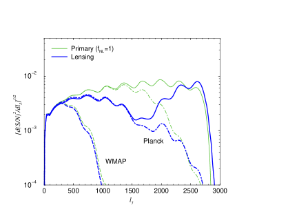
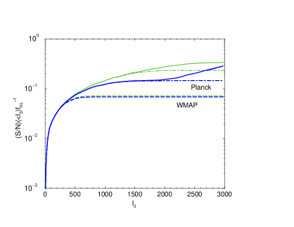
Figure 3: The signal-to-noise ratio for a detection of the CMB bispectrum with (thick lines) and without (thin lines) lensing. The long-dashed lines show the case for WMAP and dot-dashed lines for Planck. The left panel shows the signal-to-noise ratio as a function of l3subscript𝑙3l_{3}, while the right panel shows the cumulative signal-to-noise ratio below l3subscript𝑙3l_{3} in the x-axis. Note the overall reduction in the signal-to-noise ratio (when l31500similar-tosubscript𝑙31500l_{3}\sim 1500) in the case of lensing relative to the case where lensing is ignored.

Noting that the Wigner-3j𝑗j symbol obeys the identity

m1m2(l1l2l3m1m2m3)(l1l2l3′′m1m2m3′′)=δl3l3′′δm3m3′′(2l3+1),subscriptsubscript𝑚1subscript𝑚2subscript𝑙1subscript𝑙2subscript𝑙3subscript𝑚1subscript𝑚2subscript𝑚3subscript𝑙1subscript𝑙2superscriptsubscript𝑙3′′subscript𝑚1subscript𝑚2superscriptsubscript𝑚3′′subscript𝛿subscript𝑙3superscriptsubscript𝑙3′′subscript𝛿subscript𝑚3superscriptsubscript𝑚3′′2subscript𝑙31\sum_{m_{1}m_{2}}\left(\begin{array}[]{ccc}\!l_{1}\!&l_{2}\!&l_{3}\!\\ \!m_{1}\!&m_{2}\!&m_{3}\!\end{array}\right)\left(\begin{array}[]{ccc}\!l_{1}\!&l_{2}\!&l_{3}^{\prime\prime}\!\\ \!m_{1}\!&m_{2}\!&m_{3}^{\prime\prime}\!\end{array}\right)=\frac{\delta_{l_{3}l_{3}^{\prime\prime}}\delta_{m_{3}m_{3}^{\prime\prime}}}{(2l_{3}+1)}, (41)

we can re-write the lensed bispectrum as

B~l1l2l3Θsuperscriptsubscript~𝐵subscript𝑙1subscript𝑙2subscript𝑙3Θ\displaystyle\tilde{B}_{l_{1}l_{2}l_{3}}^{{\Theta}} =\displaystyle= Bl1l2l3Θ+12Bl1l2l3Θl3Cl3ϕS1+2Perm.superscriptsubscript𝐵subscript𝑙1subscript𝑙2subscript𝑙3Θ12superscriptsubscript𝐵subscript𝑙1subscript𝑙2subscript𝑙3Θsubscriptsuperscriptsubscript𝑙3superscriptsubscript𝐶superscriptsubscript𝑙3italic-ϕsubscript𝑆12Perm.\displaystyle{B}_{l_{1}l_{2}l_{3}}^{{\Theta}}+\frac{1}{2}B_{l_{1}l_{2}l_{3}}^{{\Theta}}\sum_{l_{3}^{\prime}}C_{l_{3}^{\prime}}^{\phi}S_{1}+2\;\text{Perm.} (42)
+l2′′l3′′Bl1l2′′l3′′Θl2Cl2ϕS2+2Perm.subscriptsuperscriptsubscript𝑙2′′superscriptsubscript𝑙3′′superscriptsubscript𝐵subscript𝑙1superscriptsubscript𝑙2′′superscriptsubscript𝑙3′′Θsubscriptsuperscriptsubscript𝑙2superscriptsubscript𝐶superscriptsubscript𝑙2italic-ϕsubscript𝑆22Perm.\displaystyle+\sum_{l_{2}^{\prime\prime}l_{3}^{\prime\prime}}B_{l_{1}l_{2}^{\prime\prime}l_{3}^{\prime\prime}}^{{\Theta}}\sum_{l_{2}^{\prime}}C_{l_{2}^{\prime}}^{\phi}S_{2}+2\;\text{Perm.}

where

S1=1(2l3+1)m3m3Jl3l3l3l3m3m3m3m3,andsubscript𝑆112subscript𝑙31subscriptsubscript𝑚3subscriptsuperscriptsubscript𝑚3superscriptsubscript𝐽subscript𝑙3superscriptsubscript𝑙3subscript𝑙3superscriptsubscript𝑙3subscript𝑚3superscriptsubscript𝑚3subscript𝑚3superscriptsubscript𝑚3and\displaystyle S_{1}=\frac{1}{(2l_{3}+1)}\sum_{m_{3}}\sum_{m_{3}^{\prime}}J_{l_{3}l_{3}^{\prime}l_{3}l_{3}^{\prime}}^{m_{3}m_{3}^{\prime}m_{3}m_{3}^{\prime}}\;,\;\;\text{and}
S2=m2m2′′m3′′m1m2m3(l1l2l3m1m2m3)(l1l2′′l3′′m1m2′′m3′′)subscript𝑆2subscriptsuperscriptsubscript𝑚2superscriptsubscript𝑚2′′superscriptsubscript𝑚3′′subscriptsubscript𝑚1subscript𝑚2subscript𝑚3subscript𝑙1subscript𝑙2subscript𝑙3subscript𝑚1subscript𝑚2subscript𝑚3subscript𝑙1superscriptsubscript𝑙2′′superscriptsubscript𝑙3′′subscript𝑚1superscriptsubscript𝑚2′′superscriptsubscript𝑚3′′\displaystyle S_{2}=\sum_{m_{2}^{\prime}m_{2}^{\prime\prime}m_{3}^{\prime\prime}}\sum_{m_{1}m_{2}m_{3}}\left(\begin{array}[]{ccc}\!l_{1}\!&l_{2}\!&l_{3}\!\\ \!m_{1}\!&m_{2}\!&m_{3}\!\end{array}\right)\left(\begin{array}[]{ccc}\!l_{1}\!&l_{2}^{\prime\prime}\!&l_{3}^{\prime\prime}\!\\ \!m_{1}\!&m_{2}^{\prime\prime}\!&m_{3}^{\prime\prime}\!\end{array}\right) (47)
×Il2l2l2′′m2m2m2′′Il3l2l3′′m3m2m3′′absentsuperscriptsubscript𝐼subscript𝑙2superscriptsubscript𝑙2superscriptsubscript𝑙2′′subscript𝑚2superscriptsubscript𝑚2superscriptsubscript𝑚2′′superscriptsubscript𝐼subscript𝑙3superscriptsubscript𝑙2superscriptsubscript𝑙3′′subscript𝑚3superscriptsubscript𝑚2superscriptsubscript𝑚3′′\displaystyle\hskip 99.58464pt\times I_{l_{2}l_{2}^{\prime}l_{2}^{\prime\prime}}^{m_{2}m_{2}^{\prime}m_{2}^{\prime\prime}}I_{l_{3}l_{2}^{\prime}l_{3}^{\prime\prime}}^{m_{3}m_{2}^{\prime}m_{3}^{\prime\prime}} (48)

The sum of the geometric term Jl3l3l3l3m3m3m3m3superscriptsubscript𝐽subscript𝑙3superscriptsubscript𝑙3subscript𝑙3superscriptsubscript𝑙3subscript𝑚3superscriptsubscript𝑚3subscript𝑚3superscriptsubscript𝑚3J_{l_{3}l_{3}^{\prime}l_{3}l_{3}^{\prime}}^{m_{3}m_{3}^{\prime}m_{3}m_{3}^{\prime}} over m3superscriptsubscript𝑚3m_{3}^{\prime} yields Hu00

S1=1(2l3+1)m312l3(l3+1)l3(l3+1)2l3+14π.subscript𝑆112subscript𝑙31subscriptsubscript𝑚312subscript𝑙3subscript𝑙31superscriptsubscript𝑙3superscriptsubscript𝑙312superscriptsubscript𝑙314𝜋S_{1}=-\frac{1}{(2l_{3}+1)}\sum_{m_{3}}\frac{1}{2}l_{3}(l_{3}+1)l_{3}^{\prime}(l_{3}^{\prime}+1)\frac{2l_{3}^{\prime}+1}{4\pi}\,. (49)

Hence, with summation over m3subscript𝑚3m_{3} leading to a factor (2l3+1)2subscript𝑙31(2l_{3}+1), the expression for S1subscript𝑆1S_{1} simplifies to

S1=12l3(l3+1)l3(l3+1)2l3+14π.subscript𝑆112subscript𝑙3subscript𝑙31superscriptsubscript𝑙3superscriptsubscript𝑙312superscriptsubscript𝑙314𝜋S_{1}=-\frac{1}{2}l_{3}(l_{3}+1)l_{3}^{\prime}(l_{3}^{\prime}+1)\frac{2l_{3}^{\prime}+1}{4\pi}\,. (50)
Refer to caption
Refer to caption
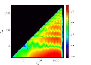
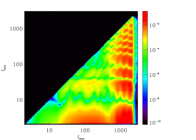
Figure 4: Contour plots of d(S/N)2/dloglmaxdloglmin𝑑superscript𝑆𝑁2𝑑subscript𝑙max𝑑subscript𝑙mind(S/N)^{2}/d\log l_{\rm max}d\log l_{\rm min} (equation 77) as a function of lmaxsubscript𝑙maxl_{\rm max} and lminsubscript𝑙minl_{\rm min} for the primary bispectrum (top panel) and the lensed primary bispectrum (bottom panel). We take fNL=1subscript𝑓NL1f_{\rm NL}=1.
Refer to caption
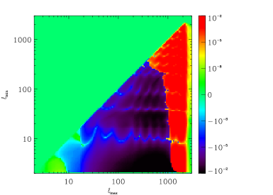
Figure 5: Contour plot of the difference d[(S/N)lensed2(S/N)unlensed2)/dloglmaxdloglmind[(S/N)^{2}_{\rm lensed}-(S/N)^{2}_{\rm unlensed})/d\log l_{\rm max}d\log l_{\rm min} as a function of lmaxsubscript𝑙maxl_{\rm max} and lminsubscript𝑙minl_{\rm min} (same as the difference between bottom and top panels of Figure 4).
Refer to caption
Figure 6: The bias in the primordial non-Gaussianity parameter fNLsubscript𝑓NLf_{\rm NL} when lensing is ignored in the estimation.(+)/(-) shows the sign of ΔfNL/fNLΔsubscript𝑓NLsubscript𝑓NL\Delta f_{\rm NL}/f_{\rm NL} between the true and measured values (see text for details).

In order to evaluate S2subscript𝑆2S_{2}, we first re-express Illl′′mmm′′superscriptsubscript𝐼𝑙superscript𝑙superscript𝑙′′𝑚superscript𝑚superscript𝑚′′I_{ll^{\prime}l^{\prime\prime}}^{mm^{\prime}m^{\prime\prime}} as

Illl′′mmm′′=flll′′(lll′′mmm′′),superscriptsubscript𝐼𝑙superscript𝑙superscript𝑙′′𝑚superscript𝑚superscript𝑚′′subscript𝑓𝑙superscript𝑙superscript𝑙′′𝑙superscript𝑙superscript𝑙′′𝑚superscript𝑚superscript𝑚′′I_{ll^{\prime}l^{\prime\prime}}^{mm^{\prime}m^{\prime\prime}}=f_{ll^{\prime}l^{\prime\prime}}\left(\begin{array}[]{ccc}\!l\!&l^{\prime}\!&l^{\prime\prime}\!\\ \!m\!&m^{\prime}\!&m^{\prime\prime}\!\end{array}\right)\,, (51)

where Hu00

flll′′=12[l(l+1)+l′′(l′′+1)l(l+1)](lll′′000).subscript𝑓𝑙superscript𝑙superscript𝑙′′12delimited-[]superscript𝑙superscript𝑙1superscript𝑙′′superscript𝑙′′1𝑙𝑙1𝑙superscript𝑙superscript𝑙′′000f_{ll^{\prime}l^{\prime\prime}}=\frac{1}{2}\bigg{[}l^{\prime}(l^{\prime}+1)+l^{\prime\prime}(l^{\prime\prime}+1)-l(l+1)\bigg{]}\left(\begin{array}[]{ccc}\!l\!&l^{\prime}\!&l^{\prime\prime}\!\\ \!0\!&0\!&0\!\end{array}\right)\,. (52)

Then the expression for S2subscript𝑆2S_{2} can be re-written as

S2subscript𝑆2\displaystyle S_{2} =\displaystyle= fl2l2l2′′fl3l2l3′′m2m2′′m3′′m1m2m3(l1l2l3m1m2m3)×\displaystyle f_{l_{2}l_{2}^{\prime}l_{2}^{\prime\prime}}\;f_{l_{3}l_{2}^{\prime}l_{3}^{\prime\prime}}\sum_{m_{2}^{\prime}m_{2}^{\prime\prime}m_{3}^{\prime\prime}}\sum_{m_{1}m_{2}m_{3}}\left(\begin{array}[]{ccc}\!l_{1}\!&l_{2}\!&l_{3}\!\\ \!m_{1}\!&m_{2}\!&m_{3}\!\end{array}\right)\times\;\; (62)
(l1l2′′l3′′m1m2′′m3′′)(l2l2l2′′m2m2m2′′)(l3l2l3′′m3m2m3′′)subscript𝑙1superscriptsubscript𝑙2′′superscriptsubscript𝑙3′′subscript𝑚1superscriptsubscript𝑚2′′superscriptsubscript𝑚3′′subscript𝑙2superscriptsubscript𝑙2superscriptsubscript𝑙2′′subscript𝑚2superscriptsubscript𝑚2superscriptsubscript𝑚2′′subscript𝑙3superscriptsubscript𝑙2superscriptsubscript𝑙3′′subscript𝑚3superscriptsubscript𝑚2superscriptsubscript𝑚3′′\displaystyle\left(\begin{array}[]{ccc}\!l_{1}\!&l_{2}^{\prime\prime}\!&l_{3}^{\prime\prime}\!\\ \!m_{1}\!&m_{2}^{\prime\prime}\!&m_{3}^{\prime\prime}\!\end{array}\right)\left(\begin{array}[]{ccc}\!l_{2}\!&l_{2}^{\prime}\!&l_{2}^{\prime\prime}\!\\ \!m_{2}\!&m_{2}^{\prime}\!&m_{2}^{\prime\prime}\!\end{array}\right)\left(\begin{array}[]{ccc}\!l_{3}\!&l_{2}^{\prime}\!&l_{3}^{\prime\prime}\!\\ \!m_{3}\!&m_{2}^{\prime}\!&m_{3}^{\prime\prime}\!\end{array}\right)
=\displaystyle= fl2l2l2′′fl3l2l3′′(1)l+l2+l3{l1l2l3l2l3′′l2′′},subscript𝑓subscript𝑙2superscriptsubscript𝑙2superscriptsubscript𝑙2′′subscript𝑓subscript𝑙3superscriptsubscript𝑙2superscriptsubscript𝑙3′′superscript1superscript𝑙superscriptsubscript𝑙2superscriptsubscript𝑙3subscript𝑙1subscript𝑙2subscript𝑙3superscriptsubscript𝑙2superscriptsubscript𝑙3′′superscriptsubscript𝑙2′′\displaystyle f_{l_{2}l_{2}^{\prime}l_{2}^{\prime\prime}}\;f_{l_{3}l_{2}^{\prime}l_{3}^{\prime\prime}}(-1)^{l^{\prime}+l_{2}^{\prime}+l_{3}^{\prime}}\left\{\begin{array}[]{ccc}l_{1}&l_{2}&l_{3}\\ l_{2}^{\prime}&l_{3}^{\prime\prime}&l_{2}^{\prime\prime}\end{array}\right\}\,, (65)

where, in the last step, we have introduced the Wigner-6j𝑗j symbol Hu01 . The values of the Wigner-6j𝑗j symbol can be computed numerically with a fast and efficient recursive algorithm Schulten .

Finally, substituting the expressions for S1subscript𝑆1S_{1} and S2subscript𝑆2S_{2} in equation (42) and including all permutations in a single expression, we can write the lensed bispectrum as

B~l1l2l3Θ=superscriptsubscript~𝐵subscript𝑙1subscript𝑙2subscript𝑙3Θabsent\displaystyle\tilde{B}_{l_{1}l_{2}l_{3}}^{{\Theta}}=
[1{l1(l1+1)+l2(l2+1)+l3(l3+1)}]Bl1l2l3Θdelimited-[]1subscript𝑙1subscript𝑙11subscript𝑙2subscript𝑙21subscript𝑙3subscript𝑙31superscriptsubscript𝐵subscript𝑙1subscript𝑙2subscript𝑙3Θ\displaystyle\bigg{[}1-\mathcal{R}\bigg{\{}l_{1}(l_{1}+1)+l_{2}(l_{2}+1)+l_{3}(l_{3}+1)\bigg{\}}\bigg{]}B_{l_{1}l_{2}l_{3}}^{{\Theta}}
+lpqClϕϕ[fl2lpfl3lq(1)n{l1l2l3lqp}Bl1pqΘ\displaystyle+\sum_{lpq}C_{l}^{\phi\phi}\bigg{[}f_{l_{2}lp}f_{l_{3}lq}(-1)^{n}\left\{\begin{array}[]{ccc}l_{1}&l_{2}&l_{3}\\ l&q&p\end{array}\right\}{B}_{l_{1}pq}^{{\Theta}} (68)
fl3lpfl1lq(1)n{l1l2l3plq}Bpl2qΘsubscript𝑓subscript𝑙3𝑙𝑝subscript𝑓subscript𝑙1𝑙𝑞superscript1𝑛subscript𝑙1subscript𝑙2subscript𝑙3𝑝𝑙𝑞superscriptsubscript𝐵𝑝subscript𝑙2𝑞Θ\displaystyle\hskip 48.36967ptf_{l_{3}lp}f_{l_{1}lq}(-1)^{n}\left\{\begin{array}[]{ccc}l_{1}&l_{2}&l_{3}\\ p&l&q\end{array}\right\}{B}_{pl_{2}q}^{{\Theta}} (71)
fl1lpfl2lq(1)n{l1l2l3qpl}Bpql3Θ]\displaystyle\hskip 48.36967ptf_{l_{1}lp}f_{l_{2}lq}(-1)^{n}\left\{\begin{array}[]{ccc}l_{1}&l_{2}&l_{3}\\ q&p&l\end{array}\right\}{B}_{pql_{3}}^{{\Theta}}\bigg{]} (74)

where

=14ll(l+1)2l+14πClϕϕ14subscript𝑙𝑙𝑙12𝑙14𝜋superscriptsubscript𝐶𝑙italic-ϕitalic-ϕ\mathcal{R}=\frac{1}{4}\sum_{l}l(l+1)\frac{2l+1}{4\pi}C_{l}^{\phi\phi} (75)

and n(l+p+q)𝑛𝑙𝑝𝑞n\equiv(l+p+q).

V Results & Discussion

We illustrate the modification to the equilateral configurations of the bispectrum in Figure 1, where we plot l4BlllΘ/(2π)2superscript𝑙4subscriptsuperscript𝐵Θ𝑙𝑙𝑙superscript2𝜋2l^{4}B^{\Theta}_{lll}/(2\pi)^{2} as a function of the multipole l𝑙l. The primary CMB bispectrum assumes fNL=1subscript𝑓NL1f_{\rm NL}=1 and is calculated with the full radiation transfer function gTl(k)subscript𝑔𝑇𝑙𝑘g_{Tl}(k). The lensing description makes use of the all-sky treatment to calculate both Clϕsuperscriptsubscript𝐶𝑙italic-ϕC_{l}^{\phi} and the lensed bispectrum. The flat-sky expression gives a result consistent with the all-sky expression at better than 5% at all multipoles if the all-sky expression for Clϕsuperscriptsubscript𝐶𝑙italic-ϕC_{l}^{\phi} is used in both calculations. The difference is at the level of 10% if the two expression make use of the two separate calculations of Clϕsuperscriptsubscript𝐶𝑙italic-ϕC_{l}^{\phi}, as in the case of the angular power spectrum Hu00 . In the case of the equilateral configurations of the bispectrum, the lensing effect can be best described as a smoothing and a decrease of the amplitude of non-Gaussianity power in the equilateral configuration of the bispectrum when l<1500𝑙1500l<1500 and a subsequent increase in the bispectrum amplitude at small angular scales.

In Figure 2, we show two squeezed configurations (l1l3l2similar-tosubscript𝑙1subscript𝑙3much-greater-thansubscript𝑙2l_{1}\sim l_{3}\gg l_{2}) of the bispectrum, with the short length fixed at either 10 (left panel) or 100 (right panel), as a function of the multipole l𝑙l of one side with the third side fixed at either l+10𝑙10l+10 or l+100𝑙100l+100. Without lensing, a comparison of Figure 1 and Figure 2 reveals a well-known result in the literature that the local type of the CMB bispectrum is dominated by squeezed configurations with one small side and two large sides for the bispectrum mode shape in the multipole space. With lensing, the amplitude of the squeezed configurations is significantly reduced when two of the sides have lengths l>1200𝑙1200l>1200 in the multipole space. This can be again described as a smoothing effect with lensing by the intervening large-scale structure; removing or “washing out” the primordial non-Gaussian signature in the CMB map at angular scales below a few arcminutes. Thus, when lensed by the large-scale structure, the primordial non-Gaussian CMB sky appears more Gaussian at arcminute scales when studying the non-Gaussianity at the three-point level. At same angular scales, however, the CMB sky appears more non-Gaussian due to lensing at the four-point level probed by the trispectrum Hu01 .

The removal of the non-Gaussianity is associated with the squeezed configurations, which dominate the overall signal-to-noise ratio for the detection of the primary bispectrum without lensing. Although non-Gaussianity is reduced for the squeezed configurations, lensing leads to an increase in the amplitude of the bispectrum for equilateral configurations where l1l2l3>1500similar-tosubscript𝑙1subscript𝑙2similar-tosubscript𝑙31500l_{1}\sim l_{2}\sim l_{3}>1500. This increase, however, is insignificant in terms of the overall signal-to-noise ratio as the contribution to the cumulative signal-to-noise coming from these configurations is lower, owing to the higher variances associated with foregrounds and instrumental noise at these angular scales.

To further quantify this statement, we plot, in Figure 3, the signal-to-noise ratio calculated as

(SN)2=l1l2l3(Bl1l2l3Θ)26Cl1totCl2totCl3tot,superscript𝑆𝑁2subscriptsubscript𝑙1subscript𝑙2subscript𝑙3superscriptsubscriptsuperscript𝐵Θsubscript𝑙1subscript𝑙2subscript𝑙326superscriptsubscript𝐶subscript𝑙1totsuperscriptsubscript𝐶subscript𝑙2totsuperscriptsubscript𝐶subscript𝑙3tot\left(\frac{S}{N}\right)^{2}=\sum_{l_{1}l_{2}l_{3}}\frac{\left(B^{\Theta}_{l_{1}l_{2}l_{3}}\right)^{2}}{6C_{l_{1}}^{\rm tot}C_{l_{2}}^{\rm tot}C_{l_{3}}^{\rm tot}}\,, (76)

where the noise variance calculation involves all contributions to the angular power spectrum with Cltot=C~l+Clsec+Nlsuperscriptsubscript𝐶𝑙totsubscript~𝐶𝑙superscriptsubscript𝐶𝑙secsubscript𝑁𝑙C_{l}^{\rm tot}=\tilde{C}_{l}+C_{l}^{\rm sec}+N_{l} where we include the lensed CMB power spectrum (C~lsubscript~𝐶𝑙\tilde{C}_{l}), secondary anisotropies (Clsecsuperscriptsubscript𝐶𝑙secC_{l}^{\rm sec}), and the noise power spectrum (Nlsubscript𝑁𝑙N_{l}) for both WMAP and Planck. For secondaries, we include the SZ power spectrum calculated with the halo model Cooray2 and make use of the noise calculations from Ref. Cooray for WMAP and Planck. For the case involving an experiment limited by the cosmic variance, we set Nl=0subscript𝑁𝑙0N_{l}=0. In the left panel of Figure 3, we plot d(S/N)2/dl3𝑑superscript𝑆𝑁2𝑑subscript𝑙3d(S/N)^{2}/dl_{3} as a function of l3subscript𝑙3l_{3}, while in the right panel we plot the cumulative signal-to-noise ratio out to l3subscript𝑙3l_{3} in the x-axis. In the case where lensing is not included, signal-to-noise ratio estimates for the bispectrum detection are consistent with previous calculations in the literature Komatsu .

With lensing, however, the signal-to-noise ratios are changed. As can be seen from the left panel of Figure 3, there is an overall reduction in the signal-to-noise ratio when l31500similar-tosubscript𝑙31500l_{3}\sim 1500. This difference comes from the previously described decrease in the amplitude of the non-Gaussianity in squeezed configurations of the bispectrum with lensing imposed. To further understand the differences in the signal-to-noise ratio of the lensed primary bispectrum, we plot, in Figure 4, the quantity

d(S/N)2dloglmaxdloglmin=lmaxlminl=lminlmax(BlminllmaxΘ)26ClmintotCltotClmaxtot,𝑑superscript𝑆𝑁2𝑑subscript𝑙max𝑑subscript𝑙minsubscript𝑙maxsubscript𝑙minsuperscriptsubscript𝑙subscript𝑙minsubscript𝑙maxsuperscriptsubscriptsuperscript𝐵Θsubscript𝑙min𝑙subscript𝑙max26superscriptsubscript𝐶subscript𝑙mintotsuperscriptsubscript𝐶𝑙totsuperscriptsubscript𝐶subscript𝑙maxtot\frac{d(S/N)^{2}}{d\log l_{\rm max}d\log l_{\rm min}}=l_{\rm max}l_{\rm min}\sum_{l=l_{\rm min}}^{l_{\rm max}}\frac{\left(B^{\Theta}_{l_{\rm min}ll_{\rm max}}\right)^{2}}{6C_{l_{\rm min}}^{\rm tot}C_{l}^{\rm tot}C_{l_{\rm max}}^{\rm tot}}\,, (77)

with two separate estimates for BΘsuperscript𝐵ΘB^{\Theta} and B~Θsuperscript~𝐵Θ\tilde{B}^{\Theta} to estimate this quantity without and with lensing, respectively. Note that the overall signal-to-noise ratio comes from integrating this quantity over the variables lmaxsubscript𝑙maxl_{\rm max} and lminsubscript𝑙minl_{\rm min} and we include the factor lmaxlminsubscript𝑙maxsubscript𝑙minl_{\rm max}l_{\rm min} to account for the logarithmic scaling. A comparison of the two panels in figure 4 reveals an overall decrease in the amplitude at l103similar-to𝑙superscript103l\sim 10^{3} in the case with the lensed primary bispectrum relative to the primary bispectrum alone.

In figure 5, we plot the difference of the two as a contour plot to show that lensing results in an overall decrease in the signal-to-noise ratio in the squeezed configurations when lmax103similar-tosubscript𝑙maxsuperscript103l_{\rm max}\sim 10^{3} and lmin<102subscript𝑙minsuperscript102l_{\rm min}<10^{2}, while there is an increase in the signal-to-noise ratio when lmax3×103similar-tosubscript𝑙max3superscript103l_{\rm max}\sim 3\times 10^{3} for all values of lminsubscript𝑙minl_{\rm min}. These plots demonstrates the same trends described with respect to figure 2 involving a decrease in the amplitude of the squeezed configurations of the lensed bispectrum. While there is a slight increase in the lensed bispectrum amplitude at l3>2000subscript𝑙32000l_{3}>2000, such small angular scales are not probed by Planck. Even in the cosmic variance limit, unfortunately, this small increase is insignificant given that at these same angular scales secondary anisotropies dominate the bispectrum noise variance. In terms of the cumulative signal-to-noise ratio values shown in figure 3, the minimum fNLsubscript𝑓NLf_{\rm NL} to detect the bispectrum with Planck and a cosmic variance limited experiment is increased by about 30% to 40% from fNL5similar-tosubscript𝑓NL5f_{\rm NL}\sim 5 for Planck to fNL7similar-tosubscript𝑓NL7f_{\rm NL}\sim 7. The cosmic variance-limited detection threshold for fNLsubscript𝑓NLf_{\rm NL} is increased from 3 to 5.

While the difference in cumulative signal-to-noise ratio seems insignificant for an experiment like WMAP, weak lensing could impact existing measurements of the non-Gaussianity parameter fNLsubscript𝑓NLf_{\rm NL} Komatsu5yr ; Yadav . To understand the lensing bias introduced to fNLsubscript𝑓NLf_{\rm NL}, we follow the discussion in Ref. Serra and note that the current estimators of the non-Gaussianity parameter use f^NL=S^primNsubscript^𝑓NLsubscript^𝑆prim𝑁\hat{f}_{\rm NL}=\frac{\hat{S}_{\rm prim}}{N} Komatsu2 ; Creminelli ; Yadav2 , with

S^prim=𝐩𝐪Bl1l2l3Θ𝒞𝐩𝐪1B^l1l2l3obssubscript^𝑆primsubscript𝐩𝐪subscriptsuperscript𝐵Θsubscript𝑙1subscript𝑙2subscript𝑙3subscriptsuperscript𝒞1𝐩𝐪subscriptsuperscript^𝐵obssuperscriptsubscript𝑙1superscriptsubscript𝑙2superscriptsubscript𝑙3\hat{S}_{\rm prim}=\sum_{{\bf p}{\bf q}}B^{\Theta}_{l_{1}l_{2}l_{3}}{\cal C}^{-1}_{{\bf p}{\bf q}}\hat{B}^{\rm obs}_{l_{1}^{\prime}l_{2}^{\prime}l_{3}^{\prime}}\, (78)

where Bl1l2l3Θsubscriptsuperscript𝐵Θsubscript𝑙1subscript𝑙2subscript𝑙3B^{\Theta}_{l_{1}l_{2}l_{3}} is the primary bispectrum, and 𝒞𝐩𝐪subscript𝒞𝐩𝐪{\cal C}_{{\bf p}{\bf q}} is the covariance matrix for bispectrum measurements involving triplets of 𝐩(l1l2l3)𝐩subscript𝑙1subscript𝑙2subscript𝑙3{\bf p}\equiv(l_{1}l_{2}l_{3}) and 𝐪(l1l2l3)𝐪superscriptsubscript𝑙1superscriptsubscript𝑙2superscriptsubscript𝑙3{\bf q}\equiv(l_{1}^{\prime}l_{2}^{\prime}l_{3}^{\prime}). This estimator is the optimal estimator for non-Gaussianity measurements, but given the complications associated with estimating the covariance, existing studies make use of a sub-optimal estimator which approximates the covariance with variance 𝒞αα1σ2(l1,l2,l3)δααsubscriptsuperscript𝒞1𝛼superscript𝛼superscript𝜎2subscript𝑙1subscript𝑙2subscript𝑙3subscript𝛿𝛼superscript𝛼{\cal C}^{-1}_{\mathbf{\alpha}\mathbf{\alpha^{\prime}}}\approx\sigma^{-2}(l_{1},l_{2},l_{3})\delta_{\mathbf{\alpha}\mathbf{\alpha^{\prime}}}, and introduces a linear term to equation (78) to minimize the variance of f^NLsubscript^𝑓NL\hat{f}_{\rm NL} Yadav2 . Note that N𝑁N is the overall normalization factor that can be calculated from equation (78) by replacing B^obssuperscript^𝐵obs\hat{B}^{\rm obs} with BΘsuperscript𝐵ΘB^{\Theta}.

While weak lensing modifies the observed bispectrum B^l1l2l3obs=fNLB~l1l2l3Θsubscriptsuperscript^𝐵obssubscript𝑙1subscript𝑙2subscript𝑙3subscript𝑓NLsubscriptsuperscript~𝐵Θsubscript𝑙1subscript𝑙2subscript𝑙3\hat{B}^{\rm obs}_{l_{1}l_{2}l_{3}}=f_{\rm NL}\tilde{B}^{\Theta}_{l_{1}l_{2}l_{3}}, existing measurements make the assumption that B^l1l2l3obs=fNLBl1l2l3Θsubscriptsuperscript^𝐵obssubscript𝑙1subscript𝑙2subscript𝑙3subscript𝑓NLsuperscriptsubscript𝐵subscript𝑙1subscript𝑙2subscript𝑙3Θ\hat{B}^{\rm obs}_{l_{1}l_{2}l_{3}}=f_{\rm NL}B_{l_{1}l_{2}l_{3}}^{\Theta}. This results in a biased estimate of f^NLsubscript^𝑓NL\hat{f}_{\rm NL} from the true value of the non-Gaussianity parameter fNLtruesubscriptsuperscript𝑓trueNLf^{\rm true}_{\rm NL}. The fractional difference of this bias Δf/f^NL(fNLtruef^NL)/f^NLΔ𝑓subscript^𝑓NLsubscriptsuperscript𝑓trueNLsubscript^𝑓NLsubscript^𝑓NL\Delta f/\hat{f}_{\rm NL}\equiv(f^{\rm true}_{\rm NL}-\hat{f}_{\rm NL})/\hat{f}_{\rm NL} can be calculated through the covariance between the lensed and unlensed CMB primary bispectrum Δf/f^NL=1[Bl1l2l3Θσ2B~l1l2l3Θ/Bl1l2l3Θσ2Bl1l2l3Θ]Δ𝑓subscript^𝑓NL1delimited-[]subscriptsuperscript𝐵Θsubscript𝑙1subscript𝑙2subscript𝑙3superscript𝜎2subscriptsuperscript~𝐵Θsubscript𝑙1subscript𝑙2subscript𝑙3subscriptsuperscript𝐵Θsubscript𝑙1subscript𝑙2subscript𝑙3superscript𝜎2subscriptsuperscript𝐵Θsubscript𝑙1subscript𝑙2subscript𝑙3\Delta f/\hat{f}_{\rm NL}=1-[\sum B^{\Theta}_{l_{1}l_{2}l_{3}}\sigma^{-2}\tilde{B}^{\Theta}_{l_{1}l_{2}l_{3}}/\sum B^{\Theta}_{l_{1}l_{2}l_{3}}\sigma^{-2}B^{\Theta}_{l_{1}l_{2}l_{3}}], where we have simply written the variance as σ2superscript𝜎2\sigma^{-2}. We plot Δf/f^NLΔ𝑓subscript^𝑓NL\Delta f/\hat{f}_{\rm NL} as a function of l𝑙l to which non-Gaussianity parameter measurements are performed in figure 6. Existing measurements with WMAP data probe out to lmax750similar-tosubscript𝑙max750l_{\rm max}\sim 750 and we find that existing estimates of fNLsubscript𝑓NLf_{\rm NL} are biased by similar-to\sim 6%. For Planck, if lensing is ignored, the bias is at the level of 30%.

This bias is not the same fractional difference in the signal-to-noise ratio that one can infer from figure 3 since the fractional difference in the signal-to-noise ratio with and without lensing involves a ratio of the form [B~l1l2l3Θσ2B~l1l2l3Θ/Bl1l2l3Θσ2Bl1l2l3Θ]delimited-[]subscriptsuperscript~𝐵Θsubscript𝑙1subscript𝑙2subscript𝑙3superscript𝜎2subscriptsuperscript~𝐵Θsubscript𝑙1subscript𝑙2subscript𝑙3subscriptsuperscript𝐵Θsubscript𝑙1subscript𝑙2subscript𝑙3superscript𝜎2subscriptsuperscript𝐵Θsubscript𝑙1subscript𝑙2subscript𝑙3[\sum\tilde{B}^{\Theta}_{l_{1}l_{2}l_{3}}\sigma^{-2}\tilde{B}^{\Theta}_{l_{1}l_{2}l_{3}}/\sum B^{\Theta}_{l_{1}l_{2}l_{3}}\sigma^{-2}B^{\Theta}_{l_{1}l_{2}l_{3}}]. Note that in future an unbiased estimate of fNLsubscript𝑓NLf_{\rm NL} can be obtained by replacing Bl1l2l3Θsubscriptsuperscript𝐵Θsubscript𝑙1subscript𝑙2subscript𝑙3B^{\Theta}_{l_{1}l_{2}l_{3}} in equation (78) with the lensed bispectrum B~l1l2l3Θsubscriptsuperscript~𝐵Θsubscript𝑙1subscript𝑙2subscript𝑙3\tilde{B}^{\Theta}_{l_{1}l_{2}l_{3}} and recalculating the normalization factor N𝑁N with the lensed primary bispectrum. Unfortunately, while without lensing the CMB primary bispectrum of the local model factorizes into two separate integrals with blLsuperscriptsubscript𝑏𝑙𝐿b_{l}^{L} and blNLsuperscriptsubscript𝑏𝑙NLb_{l}^{\rm NL} (described in Section II) , this factorizability is no longer preserved when lensed and impacts an easy estimation of the non-Gaussianity parameter with the existing estimator Komatsu2 . For Planck and other CMB experiments that can probe down to small angular scales for primordial non-Gaussianity measurements, it will be necessary to implement an estimator that accounts for the lensing effect.

To summarize the main results of this paper, we have discussed the primary CMB bispectrum generated at the last scattering surface, but observed today after it is weak lensed by the intervening large-scale structure. Unfortunately, as we have found, weak lensing leads to an overall decrease in the amplitude of non-Gaussianity with the biggest change on the squeezed configurations of the bispectrum that dominate the overall signal-to-noise ratio when studying the primordial non-Gaussianity parameter. For an experiment such as the Wilkinson Microwave Anisotropy Probe (WMAP), the modifications imposed by lensing results in an estimate of fNLsubscript𝑓NLf_{\rm NL} of the local model that is biased low by about 6%. For a high resolution experiment such as Planck, the lensing modification to the bispectrum must be accounted for when attempting to estimate the primordial non-Gaussianity. The minimum detectable value of fNLsubscript𝑓NLf_{\rm NL} for a cosmic variance limited experiment is similar-to\sim 5.

Acknowledgments

We thank participants of the recent non-Gaussianity workshop at the Perimeter Institute for helpful discussions and Alex Amblard for help with Figure 4. PS thanks Tommaso Stasi. This work was supported by NSF CAREER AST-0645427. We acknowledge the use of CMBFAST by Uros Seljak and Matias Zaldarriaga Seljak .

References

  • (1) See, e.g., U. Seljak and M. Zaldarriaga, Phys. Rev. Lett. 82, 2636 (1999); Phys. Rev. D 60, 043504 (1999); M. Zaldarriaga and U. Seljak, Phys. Rev. D 59, 123507 (1999); M. Zaldarriaga, Phys. Rev.  D 62, 063510 (2000) [arXiv:astro-ph/9910498]; M. H. Kesden, A. Cooray and M. Kamionkowski, Phys. Rev.  D 66, 083007 (2002) [arXiv:astro-ph/0208325]; C. Vale, A. Amblard and M. J. White, New Astron.  10, 1 (2004) [arXiv:astro-ph/0402004]; A. Amblard, C. Vale and M. J. White, New Astron.  9, 687 (2004) [arXiv:astro-ph/0403075]; S. Das and P. Bode, arXiv:0711.3793 [astro-ph].
  • (2) For a recent review see, A. Lewis and A. Challinor, Phys. Rept.  429, 1 (2006) [arXiv:astro-ph/0601594].
  • (3) W. Hu, Phys. Rev. D 62 043007 (2000) [arXiv:astro-ph/0001303]
  • (4) W. Hu and T. Okamoto, Astrophys. J. 574, 566 (2002) [arXiv:astro-ph/0111606]; M. Kesden, A. Cooray, and M. Kamionkowski, Phys. Rev. D 67, 123507 (2003) [arXiv:astro-ph/0302536]; C. M. Hirata and U. Seljak, Phys. Rev. D 68, 083002 (2003) [arXiv:astro-ph/0306354].
  • (5) M. Kamionkowski, A. Kosowsky, and A. Stebbins, Phys. Rev. Lett. 78, 2058 (1997) [arXiv:astro-ph/9609132]; U. Seljak and M. Zaldarriaga, Phys. Rev. Lett. 78, 2054 (1997) [arXiv:astro-ph/9609169].
  • (6) M. Kesden, A. Cooray, and M. Kamionkowski, Phys. Rev. Lett. 89, 011304 (2002) [arXiv:astro-ph/0202434]; L. Knox and Y.-S. Song, Phys. Rev. Lett. 89, 011303 [arXiv:astro-ph/0202286]; U. Seljak and C. Hirata, Phys. Rev. D 69, 043005 (2004) [arXiv:astro-ph/0310163].
  • (7) M. Zaldarriaga and U. Seljak, Phys. Rev. D 58, 023003 (1998) [arXiv:astro-ph/9803150].
  • (8) K. M. Smith, O. Zahn and O. Dore, Phys. Rev.  D 76, 043510 (2007) [arXiv:0705.3980 [astro-ph]].
  • (9) C. M. Hirata, S. Ho, N. Padmanabhan, U. Seljak and N. Bahcall, arXiv:0801.0644 [astro-ph].
  • (10) E. Komatsu and D. N. Spergel, Phys. Rev. D 63, 063002 (2001) [arXiv:astro-ph/0005036].
  • (11) M. Liguori, F. K. Hansen, E. Komatsu, S. Matarrese and A. Riotto, Phys. Rev. D 73, 043505 (2006) [arXiv:astro-ph/0509098].
  • (12) E. Komatsu et al. [WMAP Collaboration], Astrophys. J. Suppl.  148, 119 (2003) [arXiv:astro-ph/0302223].
  • (13) E. Komatsu et al. [WMAP Collaboration], arXiv:0803.0547 [astro-ph].
  • (14) A. P. S. Yadav and B. D. Wandelt, [arXiv:0712.1148].
  • (15) D. S. Salopek and J. R. Bond, Phys. Rev. D 42, 3936 (1990); ibid. 43, 1005 (1991)
  • (16) T. Falk, R. Rangarajan and M. Srednicki, Astrophys. J.  403, L1 (1993)
  • (17) A. Gangui, F. Lucchin, S. Matarrese and S. Mollerach, Astrophys. J.  430, 447 (1994)
  • (18) T. Pyne and S. M. Carroll, Phys. Rev. D 53, 2920 (1996)
  • (19) J. M. Maldacena, JHEP 0305, 013 (2003).
  • (20) V. Acquaviva, N. Bartolo, S. Matarrese and A. Riotto, Nucl. Phys. B667, 119 (2003), [arXiv:astroph-/0209156]
  • (21) N. Bartolo, S. Matarrese and A. Riotto, Phys. Rev. Lett.  93, 231301 (2004) [arXiv:astro-ph/0407505].
  • (22) N. Bartolo, E. Komatsu, S. Matarrese and A. Riotto, Phys. Rept. 402 (2004) 103-266
  • (23) E. I. Buchbinder, J. Khoury and B. A. Ovrut, arXiv:0710.5172 [hep-th].
  • (24) J. L. Lehners and P. J. Steinhardt, arXiv:0712.3779 [hep-th].
  • (25) D. M. Goldberg and D. N. Spergel, Phys. Rev.  D 59, 103002 (1999) [arXiv:astro-ph/9811251].
  • (26) A. R. Cooray and W. Hu, Astrophys. J.  534, 533 (2000) [arXiv:astro-ph/9910397].
  • (27) K. M. Smith and M. Zaldarriaga, arXiv:astro-ph/0612571.
  • (28) P. Serra and A. Cooray, arXiv:0801.3276 [astro-ph].
  • (29) D. Babich and E. Pierpaoli, arXiv:0803.1161 [astro-ph].
  • (30) E. Komatsu, D. N. Spergel and B. D. Wandelt, Astrophys. J.  634, 14 (2005) [arXiv:astro-ph/0305189].
  • (31) U. Seljak and M. Zaldarriaga, Astrophys. J.  469, 437 (1996) [arXiv:astro-ph/9603033].
  • (32) R. D. Blandford et al., Mon. Not. Roy. Astron. Soc. 251, 600 (1991); J. Miralda-Escudé, Astrophys. J. 380, 1 (1991); N. Kaiser, Astrophys. J.  388, 277 (1992); M. Bartelmann and P. Schneider, Astron. Astrophys. 259, 413 (1992). For reviews, see, M. Bartelmann and P. Schneider, Phys. Rept. 340, 291 (2001); P. Schneider Gravitational Lensing: Strong, Weak & Micro, Lecture Notes of the 33rd Saas-Fee Advanced Course, (Berlin: Springer-Verlag).
  • (33) W. Hu and A. Cooray, Phys. Rev.  D 63, 023504 (2001) [arXiv:astro-ph/0008001].
  • (34) A. R. Cooray, New Astron.  9, 173 (2004) [arXiv:astro-ph/0309301]; A. Challinor and A. Lewis, Phys. Rev.  D 71, 103010 (2005) [arXiv:astro-ph/0502425].
  • (35) W. Hu, Phys. Rev. D 64, 083005 (2001).
  • (36) K. Schulten and R. Gordon, J. Math. Phys. 16, 1971 (1975).
  • (37) A. Cooray and R. K. Sheth, Phys. Rept.  372, 1 (2002) [arXiv:astro-ph/0206508]; A. Cooray, Phys. Rev.  D 62, 103506 (2000) [arXiv:astro-ph/0005287].
  • (38) P. Creminelli, A. Nicolis, L Senatore, M. Tegmark and M. Zaldarriaga, Journal of Cosmology and Astro-Particle Physics 5, 4 (2006), [arXiv:astro-ph/0509029]
  • (39) A. P. S. Yadav, E. Komatsu, B. D. Wandelt, M. Liguori, F. K. Hansen and S. Matarrese, arXiv:0711.4933 [astro-ph].