Multifractal detrended cross-correlation analysis for two nonstationary signals

Abstract

It is ubiquitous in natural and social sciences that two variables, recorded temporally or spatially in a complex system, are cross-correlated and possess multifractal features. We propose a new method called multifractal detrended cross-correlation analysis (MF-DXA) to investigate the multifractal behaviors in the power-law cross-correlations between two records in one or higher dimensions. The method is validated with cross-correlated 1D and 2D binomial measures and multifractal random walks. Application to two financial time series is also illustrated.

Fractals and multifractals are ubiquitous in natural and social sciences Mandelbrot (1983). The most usual records of observable quantities in real world are in the form of time series and their fractal and multifractal properties have been extensively investigated. There are many methods proposed for this purpose Taqqu et al. (1995); Montanari et al. (1999). For a single nonstationary time series, the detrended fluctuation analysis (DFA) can be adopted to explore its long-range autocorrelations Peng et al. (1994); Hu et al. (2001) and multifractal features Kantelhardt et al. (2002). The DFA method can also be extended to investigate higher-dimensional fractal and multifractal measures Gu and Zhou (2006).

There are many situations that several variables are simultaneously recorded that exhibit long-range dependence or multifractal nature, such as the velocity, temperature and concentration fields in turbulent flows Meneveau et al. (1990); Schmitt et al. (1996); Beaulac and Mydlarski (2004), topographic indices and crop yield in agronomy Kravchenko et al. (2000); Zeleke and Si (2004), asset prices, indexes, and trading volumes in financial markets Ivanova and Ausloos (1999); Matia et al. (2003). Recently, a first method named detrended cross-correlation analysis (DXA) is proposed to investigate the long-range cross-correlations between two nonstationary time series, which is a generalization of the DFA method Podobnik and Stanley (2008). Here we show that the DXA method can be generalized to unveil the multifractal features of two cross-correlated signals and higher-dimensional multifractal measures. The validity and potential utility of the multifractal detrended cross-correlation analysis (MF-DXA) method is illustrated using one- and two-dimensional binomial measures, multifractal random walks (MRWs), and financial prices.

Consider two time series $\{x_{i}\}$ and $\{y_{i}\}$, where $i=1,2,\cdots,M$. Without loss of generality, we can assume that these two time series have zero means. Each time series is covered with $M_{s}=[M/s]$ non-overlapping boxes of size $s$. The profile within the $v$th box $[l_{v}+1,l_{v}+s]$, where $l_{v}=(v-1)s$, are determined to be $X_{v}(k)=\sum_{j=1}^{k}x(l_{v}+j)$ and $Y_{v}(k)=\sum_{j=1}^{k}y(l_{v}+j)$, $k=1,\cdots,s$. Assume that the local trends of $\{X_{v}(k)\}$ and $\{Y_{v}(k)\}$ are $\{\widetilde{X}_{v}(k)\}$ and $\{\widetilde{Y}_{v}(k)\}$, respectively. There are many different methods for the determination of $\widetilde{X}_{v}$ and $\widetilde{Y}_{v}$. The trend functions could be polynomials Hu et al. (2001). The detrending procedure can also be carried out nonparametrically based on the empirical mode decomposition method Wu et al. (2007). The detrended covariance of each box is calculated as follows

$$F_{v}(s)=\frac{1}{s}\sum_{k=1}^{s}\left[X_{v}(k)-\widetilde{X}_{v}(k)\right]\left[Y_{v}(k)-\widetilde{Y}_{v}(k)\right]$$ (1)

The $q$th order detrended covariance is calculated as follows

$$F_{xy}(q,s)=\left[\frac{1}{m}\sum_{v=1}^{m}F_{v}(s)^{q/2}\right]^{1/q}$$ (2)

when $q\neq 0$ and

$$F_{xy}(0,s)=\exp\left[\frac{1}{2m}\sum_{v=1}^{m}\ln F_{v}(s)\right]~{}.$$ (3)

We then expect the following scaling relation

$$F_{xy}(q,s)\sim s^{h_{xy}(q)}~{}.$$ (4)

When $X=Y$, the above method reduces to the classic multifractal DFA.

In order to test the validity of the MF-DXA method, we construct two binomial measures from the $p$-model with known analytic multifractal properties as a first example Meneveau and Sreenivasan (1987). Each multifractal signal is obtained in an iterative way. We start with the zeroth iteration $g=0$, where the data set $z(i)$ consists of one value, $z^{(0)}(1)=1$. In the $g$th iteration, the data set $\{z^{(g)}(i):i=1,2,\cdots,2^{g}\}$ is obtained from $z^{(g)}(2k+1)=pz^{(g-1)}(2k+1)$ and $z^{(g)}(2k)=(1-p)z^{(g-1)}(2k)$ for $k=1,2,\cdots,2^{g-1}$. When $g\to\infty$, $z^{(g)}(i)$ approaches to a binomial measure, whose scaling exponent function $h_{zz}(q)$ has an analytic form Halsey et al. (1986); Meneveau and Sreenivasan (1987)

$$H_{zz}(q)=1/q-\log_{2}[p^{q}+(1-p)^{q}]/q~{}.$$ (5)

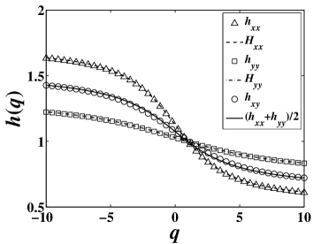
In our simulation, we have performed $g=17$ iterations with $p_{x}=0.3$ for $x(i)$ and $p_{y}=0.4$ for $y(i)$. The cross-correlation coefficient is 0.82. We find that $F_{xy}$, $F_{xx}$ and $F_{yy}$ all scale with respect to $s$ as power laws. Note that there are evident log-periodic oscillations decorating power laws, which is an inherent feature of the constructed binomial measures Sornette (1998). The best estimates of the power-law exponents are obtained when $s$ is sampled log-periodically Zhou et al. (2007). The resultant power-law exponents $h_{xy}$, $h_{xx}$ and $h_{yy}$ are illustrated in Fig. 1. The MF-DFA analysis gives $h_{xx}(q)=H_{xx}(q)$ and $h_{yy}(q)=H_{yy}(q)$. We also find that

$$h_{xy}(q)=[h_{xx}(q)+h_{yy}(q)]/2~{}.$$ (6)

For monofractal ARFIMA signals, this relation with $q=2$ is also observed Podobnik and Stanley (2008).

Figure 1: Scaling exponents $h_{xy}(q)$ estimated using the multifractal detrended cross-correlation analysis of two cross-correlated binomial measures generated from the $p$-model. The numerically estimated exponents $h_{xx}(q)$ and $h_{yy}(q)$ obtained from the multifractal detrended fluctuation analysis of $x(i)$ and $y(i)$ are also presented, which well match the analytical curves $H_{xx}(q)$ and $H_{yy}(q)$. This example illustrates the relation $h_{xy}(q)=\left[h_{xx}(q)+h_{yy}(q)\right]/2$.

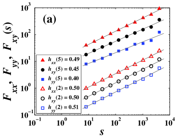
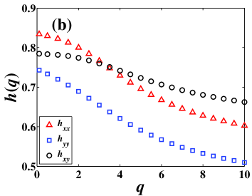
As a second example, we consider the multifractal random walks (MRWs) Bacry et al. (2001). The increments of an MRW are $\epsilon[k]e^{\omega[k]}$, where $\epsilon[k]$ and $\omega[k]$ are uncorrelated and $\omega[k]$ is a white noise. In order to generated two cross-correlated MRWs, we can generate two time series $\epsilon_{x}$ and $\epsilon_{y}$ possessing the properties in the MRW formwork and rearrange $\epsilon_{y}$ such that the rearranged series $\epsilon_{y}$ has the same rank ordering as $\epsilon_{x}$ Bogachev et al. (2007). We generate two MRW signals of size $2^{16}$ with $\lambda^{2}=0.02$ for $x(i)$ and $\lambda^{2}=0.04$ for $y(i)$, whose cross-correlation coefficient is 0.70. When $q$ is negative, no evident power-law scaling is observed for $F_{xy}(s)$, which has great fluctuations. When $q$ is positive, nice power-law scaling is observed for $F_{xy}$, $F_{xx}$ and $F_{yy}$, as illustrated in Fig. 2(a) for $q=2$ and 5. The power-law exponents $h_{xy}$, $h_{xx}$ and $h_{yy}$ are illustrated in Fig. 2(b). We see that Eq. (6) holds in repeated numerical experiments. However, this relation does not hold for some other realizations of MRWs.

Figure 2: (color online). Multifractal nature in the power-law cross-correlations of two MRWs. (a) Power-law scaling in $F_{xy}$, $F_{xx}$ and $F_{yy}$ with respect to $s$ for $q=2$ and 5; (b) Power-law exponents $h_{xy}$, $h_{xx}$ and $h_{yy}$.

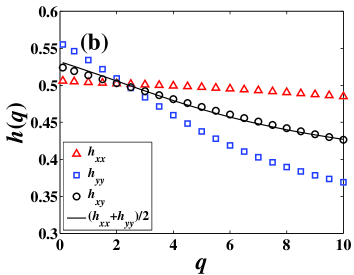
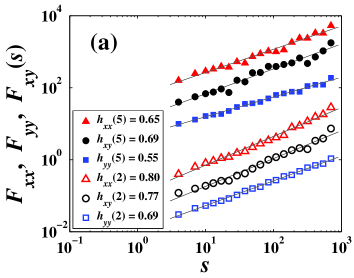
We now apply the MF-DXA method to the daily closing prices of DJIA and NASDAQ indexes. For comparison, we have used the same data sets and same scaling range as in Ref. Podobnik and Stanley (2008). No evident power-law scaling is observed for negative $q$ values. For positive $q$, we see power-law dependence of $F_{xy}$, $F_{xx}$ and $F_{yy}$ against time lag $s$. Two examples are illustrated in Fig. 3(a) for $q=2$ and 5, where the case of $q=2$ reproduces the results in Ref. Podobnik and Stanley (2008). The power-law exponents $h_{xy}$, $h_{xx}$ and $h_{yy}$ are depicted in Fig. 2(b), which are nonlinear functions with respect to $q$. We see that each time series of the absolute returns possesses multifractal nature and their power-law cross-correlations also exhibit multifractal nature.

Figure 3: (color online). Multifractal nature in the power-law cross-correlations of the absolute values of daily price changes for DJJIA and NASDAQ indexes in the period from July 1993 to November 2003. (a) Power-law scaling in $F_{xy}$, $F_{xx}$ and $F_{yy}$ with respect to $s$ for $q=2$ and 5. The scaling range is the same as in Ref. Podobnik and Stanley (2008). (b) Dependence of the power-law exponents $h_{xy}$, $h_{xx}$ and $h_{yy}$ as nonlinear functions of $q$, indicating the presence of multifractality. There is no clear relation between these exponents.

We can generalize the 1D MF-DFA to the 2D version and its extension to higher dimensions is straightforward. Consider two self-similar (or self-affine) surfaces of identical sizes, which can be denoted by two arrays $x(i,j)$ and $y(i,j)$, where $i=1,2,\cdots,M$, and $j=1,2,\cdots,N$. The surfaces are partitioned into $M_{s}\times N_{s}$ disjoint square segments of the same size $s\times s$, where $M_{s}=[M/s]$ and $N_{s}=[N/s]$. Each segment can be denoted by $x_{v,w}$ or $y_{v,w}$ such that $x_{v,w}(i,j)=x(l_{v}+i,l_{w}+j)$ and $y_{v,w}(i,j)=y(l_{v}+i,l_{w}+j)$ for $1\leqslant{i,j}\leqslant{s}$, where $l_{v}=(v-1)s$ and $l_{w}=(w-1)s$.

For each segment $x_{v,w}$ identified by $v$ and $w$, the cumulative sum $X_{v,w}(i,j)$ is calculated as follows:

$$X_{v,w}(i,j)=\sum_{k_{1}=1}^{i}\sum_{k_{2}=1}^{j}{x_{v,w}(k_{1},k_{2})}~{},$$ (7)

where $1\leqslant{i,j}\leqslant{s}$. The cumulative sum $Y_{v,w}(i,j)$ can be calculated similarly from $y_{v,w}$. The detrended covariance of the two segments can be determined as follows,

$$F_{v,w}(s)=\frac{1}{s^{2}}\sum_{i=1}^{s}\sum_{j=1}^{s}\left[X_{v,w}(i,j)-\widetilde{X}_{v,w}(i,j)\right]$$

$$\times\left[Y_{v,w}(i,j)-\widetilde{Y}_{v,w}(i,j)\right]~{}.$$ (8)

where $\widetilde{X}_{v,w}$ and $\widetilde{Y}_{v,w}$ are the local trends of $X_{v,w}$ and $Y_{v,w}$, respectively. The trend function is pre-chosen in different function forms Gu and Zhou (2006). The simplest function could be a plane $\widetilde{u}(i,j)=ai+bj+c$, which is adopted to test the validation of the method. The overall detrended cross-correlation is calculated by averaging over all the segments, that is,

$$F_{xy}(q,s)=\left\{\frac{1}{M_{s}N_{s}}\sum_{v=1}^{M_{s}}\sum_{w=1}^{N_{s}}{\left[F_{v,w}(s)\right]^{q/2}}\right\}^{1/q}~{},$$ (9)

where $q$ can take any real value except for $q=0$. When $q=0$, we have

$$F_{xy}(q,s)=\exp\left\{\frac{1}{2M_{s}N_{s}}\sum_{v=1}^{M_{s}}\sum_{w=1}^{N_{s}}{\ln[F_{v,w}(s)]}\right\}~{},$$ (10)

according to L’Hôspital’s rule. The scaling relation between the detrended fluctuation function $F_{xy}(q,s)$ and the size scale $s$ can be determined as follows

$$F_{xy}(q,s)\sim s^{h_{xy}(q)}~{}.$$ (11)

Since $N$ and $M$ need not be a multiple of the segment size $s$, two orthogonal strips at the end of the profile may remain. Taking these ending parts of the surface into consideration, the same partitioning procedure can be repeated starting from the other three corners Kantelhardt et al. (2001).

It is noteworthy to point out that the order of cumulative summation and partitioning is crucial in the analysis of two- or higher-dimensional multifractals. Consider the point located at $(l_{v}+i,l_{w}+j)$ in the box identified by $v$ and $w$, where $1\leqslant{i,j}\leqslant{s}$. The cumulative sum $X(l_{v}+i,l_{w}+j)$ can be expressed as follows

$$X(l_{v}+i,l_{w}+j)=X_{v,w}(i,j)+\sum_{k_{1}=1}^{l_{v}}\sum_{k_{2}=1}^{l_{w}}{x(k_{1},k_{2})}$$

$$+\sum_{k_{1}=1}^{l_{v}}\sum_{k_{2}=l_{w}}^{l_{w}+j}{x(k_{1},k_{2})}+\sum_{k_{1}=l_{v}}^{l_{v}+i}\sum_{k_{2}=1}^{l_{w}}{x(k_{1},k_{2})}~{}.$$ (12)

For any pair of $(i,j)$, $X_{v,w}(i,j)$ is localized to the segment $x_{v,w}$, while $X(l_{v}+i,l_{w}+j)$ contains extra information outside the segment as shown above, which is not constant for different $i$ and $j$ and thus can not be removed by the detrending procedure. We find that the power-law scaling is absent if $X(l_{v}+i,l_{w}+j)$ is used in Eq. (7). This observation is analogous to the case of higher-dimensional detrended fluctuation analysis Gu and Zhou (2006).

We now present numerical experiments validating the two-dimensional multifractal detrended cross-correlation analysis. There exist several methods for the synthesis of two-dimensional multifractal measures or multifractal rough surfaces Decoster et al. (2000). The most classic method follows a multiplicative cascading process, which can be either deterministic or stochastic Mandelbrot (1974); Meneveau and Sreenivasan (1987); Novikov (1990); Meneveau and Sreenivasan (1991). The simplest one is the $p$ model proposed to mimic the kinetic energy dissipation field in fully developed turbulence Meneveau and Sreenivasan (1987). Starting from a square, one partitions it into four sub-squares of the same size and assigns four given proportions of measure $p_{11}$, $p_{12}$, $p_{21}$, and $p_{22}$ to them. Then each sub-square is divided into four smaller squares and the measure is redistributed in the same way. This procedure is repeated $g$ times and we generate multifractal “surfaces” of size $2^{g}\times 2^{g}$. The analytical expression of $H_{xx}(q)$ or $H_{yy}(q)$ for individual multifractals is

$$H(q)=\left[2-\log_{2}\left(p_{11}^{q}+p_{12}^{q}+p_{21}^{q}+p_{22}^{q}\right)\right]/q~{}.$$ (13)

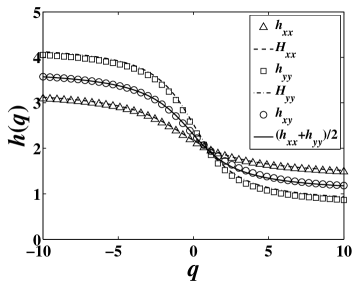
In our simulation, we have used $p_{11}=0.10$, $p_{12}=0.20$, $p_{21}=0.30$, and $p_{22}=0.40$ for $X$ and $p_{11}=0.05$, $p_{12}=0.15$, $p_{21}=0.20$, and $p_{22}=0.60$ for $Y$. We find that the cross-correlation coefficient between the two multifractals depends linearly on the generation number $g$: $c=-0.0408g+0.9528$, where the value of R-squared is 0.9997. The 95% confidence intervals for the slope and intercept are $[-0.0415,-0.0402]$ and $[0.9489,0.9566]$, respectively. In our numerical experiment, we have used $g=12$, which gives $c=0.48$. Very nice power-law behaviors are confirmed in $F_{xy}(q,s)$, $F_{xx}(q,s)$, and $F_{yy}(q,s)$ with respect to $s$ for different values of $q$. The resultant power-law exponents $h_{xy}(q)$, $h_{xx}(q)$ and $h_{yy}(q)$ are illustrated in Fig. 4 marked with open circles, squares and triangles, respectively. We find that the relation $h_{xy}(q)=\left[h_{xx}(q)+h_{yy}(q)\right]/2$ holds.

Figure 4: Multifractal detrended cross-correlation analysis of two cross-correlated synthetic binomial measures from the $p$-model. The size of each multifractal is $4096\times 4096$ and the cross-correlation coefficient is 0.48. The numerical exponents $h_{xx}(q)$ and $h_{yy}(q)$ obtained from the multifractal detrended fluctuation analysis of $X$ and $Y$ locate approximately on the analytical curves $H_{xx}(q)$ and $H_{yy}(q)$. This example illustrates the relation $h_{xy}(q)=\left[h_{xx}(q)+h_{yy}(q)\right]/2$.

In summary, we have proposed a multifractal detrended cross-correlation analysis to explore the multifractal behaviors in power-law cross-correlations between two simultaneously recorded time series or higher-dimensional signals. The MF-DXA method is a combination of multifractal analysis and detrended cross-correlation analysis. Potential fields of application include turbulence, financial markets, ecology, physiology, geophysics, and so on.