Adsorption Kinetics of a Single Polymer on a Solid Plane

Abstract

We study analytically and by means of an off-lattice bead-spring dynamic Monte Carlo simulation model the adsorption kinetics of a single macromolecule on a structureless flat substrate in the regime of strong physisorption. The underlying notion of a “stem-flower” polymer conformation, and the related mechanism of “zipping” during the adsorption process are shown to lead to a Fokker-Planck equation with reflecting boundary conditions for the time-dependent probability distribution function (PDF) of the number of adsorbed monomers. The theoretical treatment predicts that the mean fraction of adsorbed segments grows with time as a power law with a power of $(1+\nu)^{-1}$ where $\nu\approx 3/5$ is the Flory exponent. The instantaneous distribution of train lengths is predicted to follow an exponential relationship. The corresponding PDFs for loops and tails are also derived. The complete solution for the time-dependent PDF of the number of adsorbed monomers is obtained numerically from the set of discrete coupled differential equations and shown to be in perfect agreement with the Monte Carlo simulation results. In addition to homopolymer adsorption, we study also regular multiblock copolymers and random copolymers, and demonstrate that their adsorption kinetics may be considered within the same theoretical model.

I Introduction

The adsorption of polymers at equilibrium is fairly well understood from theoretical Fleer ; deGennes1 ; deGennes2 ; deGennes3 ; deGennes4 ; deGennes5 ; Eisen , computer simulation Eisen ; Sommer ; Baschnagel ; Milchev and experimental Takahashi ; Cohen points of view. On the other hand, a great deal of work exist on the polymer non-equilibrium adsorbtion of single polymer chains. One of the earliest MC - simulation along this line was implemented for single chains on the cubic lattice Konst . The authors have tested a totally irreversible adsorption model and a reversible one where a move resulting in the desorption of a segment was assigned a relative weight $\exp(\chi_{s})$ with $\chi_{s}$ being the segmental adsorption energy in units $k_{B}T$. It was found that at $\chi_{s}>2k_{B}T$ the fraction of segments in loops and trains start to deviate from their equilibrium values, i.e. the process become irreversible. Eventually at $\chi_{s}\approx 10k_{B}T$ the fraction of segments in loops and tails merges the corresponding values for the totally irreversible model.

One of the important questions concerns the scaling of the adsorption time $\tau_{\rm ads}$ with the length of the polymer chain $N$. Shaffer Shaffer has studied this problem using Monte Carlo simulatitions with the bond fluctuation model (BFM) for strong sticking energy of $10k_{B}T$. He found that the deviation in the instantaneous fraction of adsorbed monomers from its equilibrium value can be described by a simple exponential decay. During the late stages, however, the relaxation function begins to deviate from an exponential, and the relaxation slows down considerably. According to Shaffer, this might be due to artefacts of the lattice model (cf.also ref.Lai ). The main result of Shaffer Shaffer is that $\tau_{\rm ads}\sim N^{1.58}$ (for comparatively short chains $N\leq 80$).

The same scaling has been found by Ponomarev et al.Ponomar who also used the BFM for $N\leq 100$. Except the energy gain (per segment) of $\epsilon_{s}$, an activation barrier $\epsilon_{b}$ for a segment to desorb was introduced in this simulation, defining thus a ”temperature” $T_{b}\equiv k_{B}T/\epsilon_{b}$. This sets a characteristic time for the passage of a segment across the barrier $\tau_{b}=\tau_{0}\exp(1/T_{b})$. Different adsorption dynamics has then been found, depending on the ratio of $\tau_{b}$ and the Rouse time: $\tau_{b}/\tau_{R}\simeq N^{-2\nu-1}\exp(1/T_{b})$. The case $\tau_{b}/\tau_{R}\ll 1$ (at $T_{b}\geq 1$ ) corresponds to strong physisorption. On the other hand if the chain is relatively short and the barrier is high enough ($T_{b}$ is low enough) then $\tau_{b}/\tau_{R}\gg 1$, which corresponds to chemisorption. They argue that at $\tau_{b}/\tau_{R}\ll 1$ the adsorption follows a zipping mechanism whereby the chain adsorbs predominantly by means of sequential, consecutive attachment of monomers, a process that quickly erases existing loops. In this case $\tau_{\rm ads}\sim N^{1.57}$ for a SAW chain in agreement with Shaffer’s results Shaffer . In the opposite limit (chemisorption), the presence of a barrier enhances loop formation in the course of adsorption. It was shown that even a modest local barrier discourages the tendency for zipping and switches on a new mechanism involving loop formation. The scaling law in that regime reads $\tau_{\rm ads}\sim N^{\alpha}$, where the exponent $\alpha=0.8\pm 0.2$.

The irreversible chemisorption from the dilute polymer solution has been theoretically studied O'Shaughnessy_1 ; O'Shaughnessy_2 by making use of the master equation (ME) method Van_Kampen for the loops distribution function. The authors argue that the process is dominated by accelerated zipping when the sequential adsorption is disrupted by large loops formation.

For strong physisorption the simple zipping mechanism, as opposed to the accelerated zipping, has been also recently considered by Descas, Sommer and Blumen Descas . The authors Descas used the BFM and suggested a simple theoretical description of the corresponding adsorption dynamics based on what they call a “stem - corona” model. This leads to the scaling prediction, $\tau_{\rm ads}\sim N^{1+\nu}$, which is in reasonably good agreement with the simulation result.

In the present paper we study the case of strong physisorption by means of an off-lattice dynamic MC method and theoretically by employing the ME-formalism. This makes it possible to describe the adsorption dynamics not only in terms of the average fraction of adsorbed segments but also to include train and tail distribution functions which furnish the main constituents of the dynamic adsorption theory. Section II starts with the description of the adsorption dynamics model which shares many common features with the one suggested by Descas et al. Descas . Then we use this model within the ME-formalism to treat the time evolution of the distribution of adsorbed monomers (as well as the distributions of the monomers forming trains and tails). It is shown that the problem can be mapped onto a drift-diffusion process governed by a Fokker-Planck equation. We obtain the numerical solution of this equation and discuss its consequences. In Section III we briefly introduce the MC model. The MC-simulation results for homopolymers as well as for block- and random - copolymers in the regime of strong adsorption are given in Section IV. We show that our MC-findings are in good agreement with the theoretical predictions. We summarize our results and conclusions in Section V. Some details of the train distribution function calculation are relegated to the Appendix.

II Adsorption dynamics in terms of train and tail distributions

Consider a single polymer molecule (grafted with one end to a flat structureless surface) in an adsorption experiment which is repeated over and over again. The monomer - surface interaction is considered attractive with a sticking energy $\epsilon=E_{1}-E_{2}$, where $E_{1}$ and $E_{2}$ are respectively the monomer energies before and after the adsorption event.

II.1 Stem-flower scenario: A macroscopic law

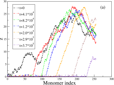
As indicated by earlier MC-simulation results Ponomar ; Descas , in the strong physisorption regime the process is assumed to follow a simple zipping mechanism. Figure  1a gives snapshots of the chain conformation as it is evident from our simulation results. One can see that the chain conformation can be considered within the framework of a “stem-flower” picture which was discussed first by Brochard-Wyart Brochard as characteristic for a polymer chain under strong stationary flow. Recently the “stem-flower” picture was employed in the case of non-stationary pulled polymer chain Sakaure . It should be pointed out that this picture shares many common features with the ”stem-corona” model, suggested by Descas et al Descas . Here we reconsider it in a more systematic way and employ it as a basic model to include fluctuations within the ME - formalism.

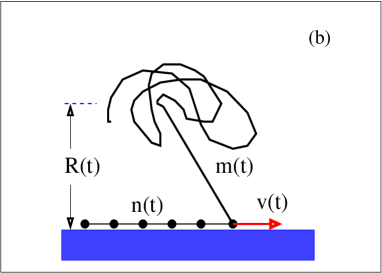
Fig. 1b presents schematically the stem-flower scenario of the adsorption dynamics. The number of adsorbed monomers at time $t$ is denoted by $n(t)$. The nonadsorbed fraction of the chain is subdivided into two parts: a stretched part (”stem”) of length $m(t)$, and a remaining part (”flower”) which is yet not affected by the tensile force of the substrate. The tensile force propagation front is at distance $R(t)$ from the surface. The rate of adsorbtion is denoted as $v(t)=a\frac{dn(t)}{dt}$, where $a$ is the chain (Kuhn) segment length.

Figure 1: (a) Snapshots of an $N=256$ chain conformation, taken at successive time moments during the adsorption process. The $z$-coordinate of the $i$-th monomer is plotted against monomer index $i$. (b) Stem-flower picture of the adsorption dynamics. The total number of adsorbed monomers at time $t$ is denoted by $n(t)$. The tail which, contains all nonadsorbed monomers, consists of a stretched part, a “stem”, of length $m(t)$, and of a nonperturbed part which is referred to as “flower”. The rate of adsorption is $v(t)$. The distance between the surface and the front of the tension propagation is $R(t)$.

A single adsorption event occurs with energy gain $\epsilon$ and entropy loss $\ln(\mu_{3}/\mu_{2})$, where $\mu_{3}$ and $\mu_{2}$ are the connectivity constants in three and two dimensions, respectively Vanderzande . In result, the driving force for adsorption can be expressed as

$$f_{\rm drive}=\frac{\epsilon-k_{B}T\ln(\mu_{3}/\mu_{2})}{a}=\frac{F}{a}$$ (1)

where $F=\epsilon-k_{B}T\ln(\mu_{3}/\mu_{2})$ is the change in free energy. The friction force is related to the pulling of the stem at rate $v(t)$, i.e.

$$f_{\rm fric}=\zeta_{0}\>a\>m(t)\>\frac{dn(t)}{dt}$$ (2)

where $\zeta_{0}$ is the Stokes friction coefficient of a single bead. The equation of motion follows from the balance of driving, $f_{\rm drive}$, and drag force, $f_{\rm fric}$, which yields

$$\zeta_{0}\>\>m(t)\>\frac{dn(t)}{dt}=\frac{F}{a^{2}}$$ (3)

One may express $m(t)$ in terms of $n(t)$, if one assumes that at time $t$ the ”flower” (which is placed on average at a distance $R(t)$ from the surface) is not affected by the tensile force. This means that $R(t)$ is the size which the chain portion $n(t)+m(t)$ occupied before the adsorption has started, i.e.,

$$a\left[n(t)+m(t)\right]^{\nu}=R(t)$$ (4)

where $\nu$ is the Flory exponent (e.g., $\nu=3/5$ in $d=3$-dimensions) Vanderzande . On the other hand, as shown in Fig. 1b,

$$a\>m(t)\approx R(t)$$ (5)

up to a geometrical factor of order unity. Therefore the relation between $m(t)$ and $n(t)$ is given as

$$n(t)\simeq m(t)^{1/\nu}-m(t)$$ (6)

During most of the adsorption process the stem is sufficiently long, $m(t)\gg 1$, so that $m(t)^{5/3}\gg m(t)$, i.e., $m(t)\simeq n(t)^{\nu}$ and Eq.(3) becomes

$$\zeta_{0}\>n(t)^{\nu}\>\frac{dn(t)}{dt}=\frac{F}{a^{2}}$$ (7)

The solution of Eq. (7) reads

$$n(t)\propto\left[\frac{F}{a^{2}\zeta_{0}}\>t\right]^{1/(1+\nu)}$$ (8)

In result, (for $d=3$ where $\nu=3/5$) one obtains a law for the adsorption kinetics, $n(t)\propto t^{0.62}$, which is in a good agreement with MC-findings Shaffer ; Ponomar ; Descas . In the course of adsorption the “stem” grows and the “flower” moves farther away from the surface. This, as it was mentioned in ref.Descas , makes the nucleation of a new adsorption site on the surface less probable.

In the late stages of adsorption the ”flower” has been largely consumed and vanishes so that the non-adsorbed part of the macromolecule exists as a ”stem” only. From this moment on the closure relation reads

$$n(t)+m(t)=N$$ (9)

Comparison of Eq. (9) with Eq. (6) shows that this pure ”stem” regime starts at $n(t)\geq N-N^{\nu}\approx N$, i.e., it could be basically neglected for sufficiently long chains.

The stem-flower scenario which we used in this section as well as the macroscopic equation of motion, eq.(7), are employed below as a starting point for the treatment of fluctuations.

II.2 Time evolution of the distribution of adsorbed monomers

Next we focus on the instantaneous number of adsorbed monomers (i.e., the total train length) distribution function $P(n,t)$. The number of adsorbed monomers $n$ and the number monomers in the nonadsorbed chain tail $l$ are mutually complementary, if one neglects the loops (we will argue below that in the strong adsorption regime the loop contribution is rather small and reduces mainly to loops of size unity). With this assumption, the corresponding tail distribution function $T(l,t)$ reads

$$T(l,t)=P(N-l,t).$$ (10)

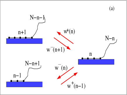
Both $P(n,t)$ and $T(l,t)$ can be obtained either from the simulation or by solving a set of coupled kinetic equations. For the latter we use the method of the Master Equation Van_Kampen . We treat the adsorption as a sequence of elementary events, describing the (un)zipping dynamics while keeping in mind that within an elementary time interval only one monomer may change its state of sorption. Thus one can treat the (un)zipping dynamics as an one-step process, shown schematically in Fig. 2a.

In order to specify the rate constants, we use the detailed balance condition Van_Kampen which in our case (cf. Fig. 2a) reads

$$\frac{w^{+}(n-1)}{w^{-}(n)}={\rm e}^{F/k_{B}T}$$ (11)

where again $F=\epsilon-k_{B}T\ln(\mu_{3}/\mu_{2})$ is the free energy win upon a monomer adsorption event and the energy gain $\epsilon=E_{1}-E_{2}$. Detailed balance condition Eq. (11) is, of course, an approximation for the non-equilibrium adsorption process in question. This implies that, despite the global non-equilibrium, close to a “touch-down” point the monomers are in local equilibrium with respect to adsorption-desorption events. This also means that the monomer size is small enough as compared to the “stem” length, so that this approximation is a good one, compatible with the “stem-flower” picture of adsorption dynamics.

Figure 2: (a) Creation - annihilation of an adsorption state with $n$-monomers due to a single-step process. The arrows indicate possible single-step transitions with $w^{+}(n)$ and $w^{-}(n)$ being the rate constants of adsorption and desorption events, respectively. (b) The adsorbed monomers form trains, divided by defects (loops of length unity). The total number of adsorbed monomers at time $t$ is denoted by $n(t)$. The train length, $h$, itself is a random number, subject to an exponential distribution $D(h,t)$ - Eq.(32).

The detailed balance requirement fixes only the ratio of the rate constants and does not fully determine their values which could be chosen as

$$w^{-}(n) = q[m(n)]\>{\rm e}^{-F/k_{B}T}$$

$$w^{+}(n-1) = q[m(n)].$$ (12)

In Eq. 12 the transmission factor $q[m(n)]$ is determined by the friction coefficient $\zeta$ which, within our stem-flower model, is defined as $\zeta=\zeta_{0}m$. Therefore, one obtains

$$q[m(n)]=\frac{k_{B}T}{a^{2}\zeta}=\frac{k_{B}T}{a^{2}\zeta_{0}\>m}.$$ (13)

The notation $q[m(n)]$ implies that the stem length $m$ depends on the total train length $n$ and, furthermore, the relationship $m(n)$ is given by the closure Eq. (6) which also holds for the instantaneous values, i.e.,

$$n\simeq m^{1/\nu}-m$$ (14)

With the rate constants from Eq. 12 at hand, the one-step master equation reads Van_Kampen

$$\frac{d}{dt}\>P(n,t) = w^{-}(n+1)\>P(n+1,t)+w^{+}(n-1)\>P(n-1,t)$$ (15)

$$- w^{+}(n)\>P(n,t)-w^{-}(n)\>P(n,t)$$

or, in a more compact form

$$\frac{d}{dt}\>P(n,t)=\Delta\left[w^{-}(n)\>P(n,t)\right]+\Delta^{-1}\left[w^{+}(n)\>P(n,t)\right]$$ (16)

where the finite-difference operators $\Delta,\;\Delta^{-1}$ are defined as

$$\Delta f(n) \equiv f(n+1)-f(n)$$

$$\Delta^{-1}f(n) \equiv f(n-1)-f(n)$$ (17)

The total number of the adsorbed monomers varies between $1$ and $N$, i.e., $1\leq n\leq N$. For $n=1$ the Eq. (15) has to be replaced by

$$\frac{d}{dt}P(1,t)=w^{-}(2)P(2,t)-w^{+}(1)P(1,t)$$ (18)

Similarly, for $n=N$ the ME reads

$$\frac{d}{dt}P(N,t)=w^{+}(N-1)P(N-1,t)-w^{-}(N)P(N,t)$$ (19)

Finally, the set of master equations (15), (18) and (19) should be supplemented by the initial condition

$$P(n,t=0)=\delta(n-1)$$ (20)

because the adsorbtion starts from the state of a one chain end grafted at the surface.

The equation of motion for the first statistical moment, $\left\langle n\right\rangle=\sum_{n=1}^{\infty}nP(n,t)$, can be obtained from Eq. (16) by performing the summation by parts:

$$\sum_{n=0}^{N-1}\>g(n)\Delta\>f(n)=g(N)f(N)-g(0)f(0)+\sum_{n=1}^{N}\>f(n)\Delta^{-1}g(n)$$ (21)

where $f(n)$ and $g(n)$ are arbitrary functions. Taking this into account and keeping in mind that $P(N,t)=P(0,t)=0$ for simplicity, the equation of motion for $\left\langle n\right\rangle$ then yields

$$\frac{d}{dt}\>\left\langle n\right\rangle=-\left\langle w^{-}(n)\right\rangle+\left\langle w^{+}(n)\right\rangle$$ (22)

With the relations for the rate constants, Eqs. (12) and 13, this equation of motion becomes

$$\zeta_{0}\>m(t)\>\frac{d}{dt}\>n(t)=\frac{k_{B}T}{a^{2}}\>\left[1-{\rm e}^{-F/k_{B}T}\right]$$ (23)

where for brevity we use the notations $n(t)=\left<n\right>$ and $m(t)=\left<m\right>$. The result, Eq. (23), should be compared with Eq. (3) derived earlier by means of a simplified physical consideration (see also paper Descas where this result was obtained before us). Formally, Eq. (23) transforms back into Eq. (3) when adsorption is very weak, $F/k_{B}T\ll 1$. Importantly, Eq. (23) has the same structure as Eq. (3) even when the adsorption is not weak and the quantity $F/k_{B}T$ is not small; the only difference between these equations is that the effective force in Eq. (23) has the form $\left(k_{B}T/a\right)\left[1-e^{-F/k_{B}T}\right]$ instead of just $F/a$. This can be understood by the analogy with the second virial coefficient of interaction between the monomer and the surface. Indeed, we know that the contribution to the free energy of an imperfect gas due to pair collisions is proportional to the second virial coefficient rather than just interaction energy; similarly in the case of adsorption, the effective second virial coefficient is the quantity that describes the effect of monomer attraction to the wall. Thus, the zipping as a strongly non-equilibrium process can not be treated quasi-statically by making use of a simple “force-ballance”. The inclusion of fluctuations by employing the ME-formalism is important in order to obtain the correct result for the driving force.

II.2.1 Fokker - Planck equation and boundary conditions

It is instructive to change now from the discrete representation, Eqs. (16), (18) and (19), to a continuous one, namely, to the Fokker-Planck equation for the distribution function $P(n,t)$ with proper boundary conditions. This can be done by the substitution

$$\Delta \simeq \frac{\partial}{\partial n}+\frac{1}{2}\frac{\partial^{2}}{\partial n^{2}}$$

$$\Delta^{-1} \simeq -\frac{\partial}{\partial n}+\frac{1}{2}\frac{\partial^{2}}{\partial n^{2}}$$ (24)

After that, Eq.(16) takes on the form

$$\frac{\partial}{\partial t}\>P(n,t)=\frac{\partial}{\partial n}\left\{\left[w^{-}(n)-w^{+}(n)\right]\>P(n,t)\right\}+\frac{1}{2}\frac{\partial^{2}}{\partial n^{2}}\left\{\left[w^{-}(n)+w^{+}(n)\right]\>P(n,t)\right\}$$ (25)

where $\left[w^{+}(n)-w^{-}(n)\right]$ and $\left[w^{-}(n)+w^{+}(n)\right]/2$ play the roles of drift velocity and diffusion coefficient, respectively.

To derive the proper boundary conditions we recall that at $n=1$ the ME has a different form, given by Eq.(18). It is convenient to require that Eq. (15) is still valid with the additional condition

$$\left[w^{+}(n-1)P(n-1,t)-w^{-}(n)P(n,t)\right]_{n=1}=0$$ (26)

i.e., the transitions between a fictitious state $n=0$ and the state $n=1$ are also balanced.

Similarly, to reconcile the equation at $n=N$, given by Eq. (19), with the general ME, Eq. (15), one should impose the condition

$$\left[w^{-}(n+1)P(n+1,t)-w^{+}(n)P(n,t)\right]_{n=N}=0$$ (27)

which again expresses the balance between an artificial state $n=N+1$ and the state $n=N$.

In order to gain a deeper insight into the boundary conditions given by Eqs.(26) and (27) let us represent Eq. (15) in the form

$$\frac{d}{dt}P(n,t)=\Delta\left[w^{-}(n)P(n,t)-w^{+}(n-1)P(n-1,t)\right]$$ (28)

This representation looks like a discrete version of the continuity equation, stating that the value in the square brackets is the probability current (with a negative sign), i.e.,

$$J(n)=w^{+}(n-1)P(n-1,t)-w^{-}(n)P(n,t)$$ (29)

A comparison of Eq. (29) with Eqs. (26) and (27) allows one to conclude that

$$J(n=1)=0\qquad\mbox{and}\qquad J(n=N+1)=0$$ (30)

i.e., one should impose reflecting boundary conditions on both ends of the interval.

Within the Fokker-Planck formalism the probability current has the form

$$J(n)=\left[w^{+}(n)-w^{-}(n)\right]P(n,t)-\frac{1}{2}\>\frac{\partial}{\partial n}\>\left\{\left[w^{+}(n)+w^{-}(n)\right]P(n,t)\right\}$$ (31)

Thus the Fokker-Planck formalism makes it possible to map the strong adsorption case onto a one-dimensional random walk problem with drift and diffusion coefficients given in terms of rate constants, Eq. (25). While such a description provides physical insight into the problem, from the viewpoint of numerics it is much easier to deal with the ME discrete set Eqs. (15), (18) and (19). We will discuss the results of this solution in Sec. II D.

II.3 Train distribution

Our MC-simulation results show that the distribution of loops in case of strong physisorption is mainly dominated by the shortest loops of length unity. These loops can be considered as defects during the process of zipping. Moreover, this distribution sets on much faster than the time for complete adsorption. Thus one may consider the total number of the adsorbed monomers $n(t)$ as a slow variable in comparison to the number of defects (or loops of length unity). The adsorbed monomers can be seen as an array of trains, separated by an equilibrium number of defects (see Fig. 2b). The partition function of this one-dimensional array can be determined rigorously (see Appendix A). Thus, one derives an expression for the train distribution function

$$D(h,t)=\frac{1}{h_{\rm av}(t)}\>\exp\left[-\frac{h}{h_{\rm av}(t)}\right]$$ (32)

where $h_{\rm av}(t)$ is the average train length. Eq.(32) is nothing but the Flory-Schulz distribution which usually governs the molecular weight distribution in equilibrium polymerization of a broad class of systems, referred to as living polymersGreer .

II.4 Results from the ME numerical solution

The set of ordinary differential equations (15), (18) and (19) with the initial condition, Eq.(20), has been solved numerically in this investigation. Typically, we use a chain length $N=32$, the total time interval takes $300$ units of the the elementary time $\tau_{0}=a^{2}\zeta_{0}/k_{B}T$, the sticking energy was chosen (in units of $k_{B}T$) as $\epsilon=4.0$, whereas the entropy loss $\ln(\mu_{3}/\mu_{2})=\ln 2$. Figure 3 demonstrates the result of this solution.

Figure 3: Adsorbed monomer number distribution function $P(n,t)$ (a) and its isolines as a $2$-dimensional log-log plot (b). The variation of the distribution maximum, $n_{max}(t)$, is a straight (dashed) line with slope $0.63$.

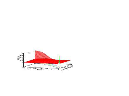
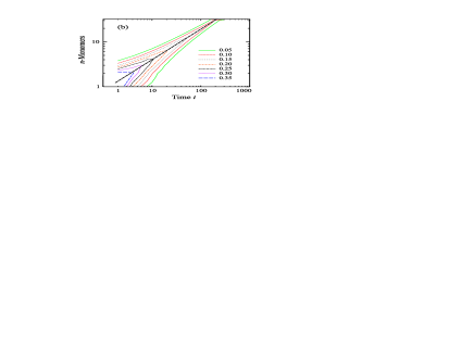
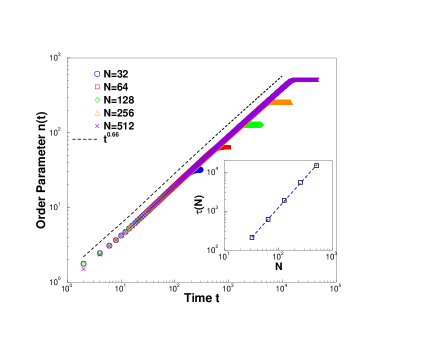
As it can be seen from Fig.3, the adsorbtion kinetics follows indeed the drift - diffusion picture. The initial distribution is very narrow: the adsorption starts with $n(0)=1$ as a grafted chain configuration. As time goes by, the distribution maximum moves to larger adsorbed monomer numbers and the distribution itself broadens. Eventually, the random process hits the boundary $n=N$ and stays there due to drift and the reflecting boundary conditions. As a result, the final distribution is a very narrow again, and is concentrated around the boundary $n=N$. It is of interest that in the double logarithmic coordinates the distribution maximum follows a straight line (cf. Fig. 3 right panel) which reveals a clear scaling law. The first moment $n(t)$ of the distribution function $P(n,t)$ also exhibits well expressed scaling behavior, $n(t)\sim t^{0.66}$, as shown in Fig. 4. In the inset we also show the resulting relationship for the time of adsorption, $\tau\propto N^{1.6}$, as expected from Eq. 8. Based on the numerical results for $P(n,t)$ and making use the relation, Eq. (10), one can calculate the tail distribution function $T(l,t)$ as well. We will discuss this in Sec. III where we present our MC-results. There it will be seen that our MC-findings are in a good agreement with these theoretical predictions.

Figure 4: The average adsorbed number of monomer vs. time for different chain lengths $N$. Dashed line denotes the slope, $t^{0.66}$, following from Eq. 8. In the inset we show the resulting scaling of the adsorption time with chain length, $\tau\propto N^{1.6}$.

III Monte Carlo Simulation Model

To check the theoretical predictions mentioned in the previous sections we have performed Monte Carlo simulations and investigated the adsorption kinetics of a homopolymer, multi-block copolymers, and random copolymers on flat surfaces. We have used a coarse grained off-lattice bead spring modelAMKB to describe the polymer chains. Our system consists of a single chain tethered at one end to a flat structureless surface. There are two kinds of monomers: ”A” and ”B”, of which only the ”A” type feels an attraction to the surface. The surface interaction of the ”A” type monomers is described by a square well potential $U_{w}(z)=\epsilon$ for $z<\delta$ and $U_{w}(z)=0$ otherwise. Here $\epsilon/k_{B}T$ is varied from $2.5$ to $10.0$. The effective bonded interaction is described by the FENE (finitely extensible nonlinear elastic) potential.

$$U_{FENE}=-K(1-l_{0})^{2}\ln\left[1-\left(\frac{l-l_{0}}{l_{max}-l_{0}}\right)^{2}\right]$$ (33)

with $K=20,l_{max}=1,l_{0}=0.7,l_{min}=0.4$

The nonbonded interactions are described by the Morse potential.

$$\frac{U_{M}(r)}{\epsilon_{M}}=\exp(-2\alpha(r-r_{min}))-2\exp(-\alpha(r-r_{min}))$$ (34)

with $\alpha=24,\;r_{min}=0.8,\;\epsilon_{M}/k_{B}T=1$.

We use periodic boundary conditions in the $x-y$ directions and impenetrable walls in the $z$ direction. We have studied polymer chains of lengths $32$, $64$, $128$, $256$ and $512$. Apart from homopolymers, we have also studied copolymer chains with block size $M=1\div 16$ and random copolymers (with a fraction of attractive monomers, $p=0.25,\;0.5,\;0.75$). The size of the box was $64\times 64\times 64$ in all cases except for the $512$ chains where we used a larger box size of $128\times 128\times 128$. The standard Metropolis algorithm was employed to govern the moves with self avoidance automatically incorporated in the potentials. In each Monte Carlo update, a monomer was chosen at random and a random displacement attempted with $\Delta x,\;\Delta y,\;\Delta z$ chosen uniformly from the interval $-0.5\leq\Delta x,\Delta y,\Delta z\leq 0.5$. The transition probability for the attempted move was calculated from the change $\Delta U$ of the potential energies before and after the move as $W=\exp(-\Delta U/k_{B}T)$. As for a standard Metropolis algorithm, the attempted move was accepted if $W$ exceeds a random number uniformly distributed in the interval $[0,1)$. A Monte Carlo Step (MCS) is elapsed when all $N$ monomers of the chain are selected at random, and given the chance to perform an elementary move. Before the surface adsorption potential is switched on, the polymer chain is equilibrated by the MC method for a period of about $10^{6}$ MCS (depending on the chain length $N$ this period is varied) whereupon one performs $200$ measurement runs, each of length $8\times 10^{6}$ MCS. In the case of random copolymers, for a given composition, i.e., percentage $p$ of the $A-$monomers, we create a new polymer chain in the beginning of the simulation run by means of a randomly chosen sequence of segments. This chain is then sampled during the course of the run, and replaced by a new sequence in the beginning of the next run.

IV Monte Carlo Simulation Results

We present here the main results from the computer simulation of the adsorption kinetics and compare them to those from the solution of the Master Equation, Eqs. (15), (18) and (19), validating thus the theoretical picture of Section II.

IV.1 Order Parameter Kinetics - homopolymers

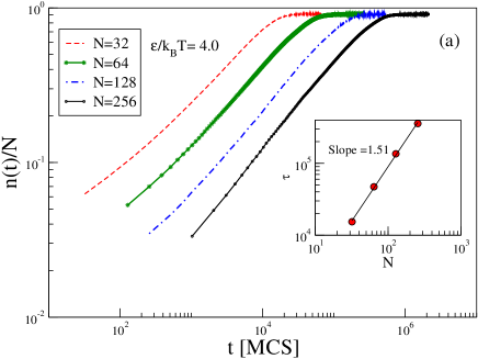
In Fig. 5a we show the adsorption time transients which describe the time variation of the order parameter $n(t)/N$ (the fraction of adsorbed segments) for homopolymer chains of different length $N$ and strong adhesion $\epsilon/k_{B}T=4.0$. Evidently, in log-log coordinates these transients appear as straight lines, suggesting that the time evolution of the adsorption process is governed by a power law. As the chain length $N$ is increased, the slope of the curves grows steadily, and for length $N=256$ it is equal to $\approx 0.56$. This value is close to the theoretically expected slope of $(1+\nu)^{-1}\approx 0.62$ - cf. Eq. 8, and for even longer lengths of the polymers would most probably be observed. The total time $\tau$ it takes a polymer chain to be fully adsorbed can be determined from the intersection of the respective late time plateau of each transient with the straight line tangent to this transient. Thus one may check the scaling of $\tau$ with polymer length $N$. In the inset to Fig. 5a we show the observed scaling of the adsorption time with chain length, $\tau\propto N^{\alpha}$ whereby the observed power ${\alpha\approx 1.51}$ is again somewhat smaller than the expected one $1+\nu\approx 1.59$. This small discrepancy is most probably due to finite-size effects too.

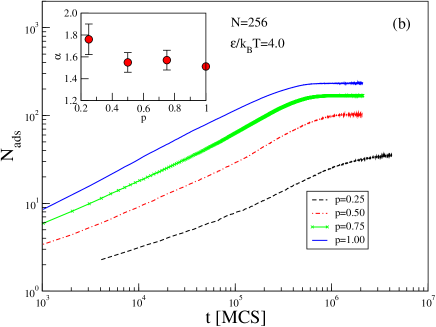
Fig. 5b presents the adsorption transients for a chain of constant length, $N=256$, for different strength of the surface potential. Evidently, as the surface potential gets stronger, the final (equilibrium) values of the transients at late times $t\rightarrow\infty$ grow while the curves are horizontally shifted to shorter times. Notwithstanding, the slope of the $n(t)$ curves remains unchanged when $\epsilon/k_{B}T$ is varied, suggesting that the kinetics of the process is well described by the assumed zipping mechanism.

Figure 5: (a) Time evolution of the order parameter (fraction of adsorbed segments) for four different chain lengths $N=32,\;64,\;128,\;\mbox{and}\;256$ at surface potential $\epsilon/k_{B}T=4.0$. The slope of the $N=256$-curve is $0.56$. The inset shows the scaling of the adsorption time with chain length,$\tau\propto N^{1.51}$. The time $\tau$ is determined from the intersection point of the late time plateau with the tangent $t^{0.56}$ to the respective $n(t)$-curve. (b) Adsorption kinetics for different strengths $\epsilon$ of the surface potential. The variation of the plateau height (i.e., the fraction of adsorbed monomers at equilibrium) with $\epsilon$ is depicted in the upper inset where the solid line $n_{t\rightarrow\infty}=1-5\exp\left(-\frac{\epsilon}{k_{B}T}\right)$ describes the equilibrium number of defects (vacancies). The lower inset shows a collapse of the adsorption transients on a single ’master curve’, if the time axis is rescaled appropriately.

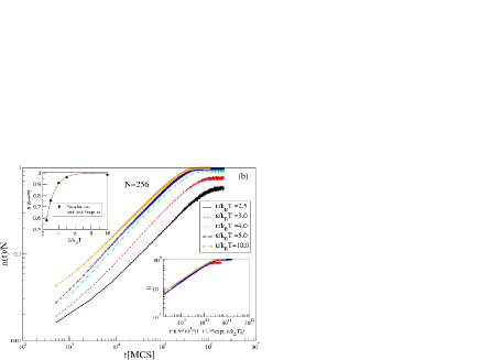
The changing plateau height may readily be understood as reflecting the correction in the equilibrium fraction of adsorbed monomers due to the presence of defects (vacancies) for any given value of $\epsilon/k_{B}T$. This is demonstrated in the upper left inset in Fig. 5b where the observed plateau values are shown to be perfectly described by the expression $n_{t\rightarrow\infty}=1-5\exp\left(-\frac{\epsilon}{k_{B}T}\right)$ under the assumption that the probability of a monomer to desorb from the surface (and create a vacancy in the train) is determined by the Boltzmann factor $\exp\frac{-\epsilon}{k_{B}T}$. Evidently, the factor of $5$ in front of the exponent yields the entropic gain in free energy when an adsorbed monomer detaches from the surface while its nearest neighbors still stick to it.

The second inset in Fig. 5b shows that the adsorption time transients collapse on a master curve, if one rescales the time axis appropriately. Note that for a very strong potential, $\epsilon/K_{B}T=10.0$, the corresponding transient deviates somewhat from the master curve since the establishment of local equilibrium (which we assumed in the theory to happen much faster than the adsorption process itself) is hampered. Also the transient for $\epsilon/k_{B}T=2.5$ (not shown in this inset) was found not to fit into the master curve since this strength is close to that of the critical threshold for adsorption, the attraction to the surface is comparatively weak and zipping is not the adequate mechanism. For the transients which do collapse on a master curve, however, one may view the rescaling of the time axis in Fig. 5b by the expression $t\rightarrow t[1-13.7\exp\frac{-\epsilon}{k_{B}T}]$ as a direct confirmation of Eq. 23 where the time variable $t$ may be rescaled with the driving force of the process (i.e., with the expression in square brackets). The factor $\approx 13.7$ gives then the ratio $\mu_{3}/\mu_{2}$ of the effective coordination numbers in $3$- and $2$-dimensions of a polymer chain with excluded volume interactions. $\mu_{3}$ and $\mu_{2}$ are model-dependent and characterize, therefore, our off-lattice model.

IV.2 Order Parameter Kinetics - regular and random copolymers

In Fig. 6 we examine the adsorption kinetics for the case of regular block copolymers with block size $M$ - Fig. 6a, and for random copolymers - Fig. 6b, bearing in mind that the zipping mechanism, assumed in our theoretical treatment, is by no means self-evident when the file of sticking $A$-monomers is interrupted by neutral $B$ segments. It becomes evident from Fig. 6a, however, that, except for a characteristic ’shoulder’ in the adsorption transients, the power-law character of the order parameter variation with time remains unchanged. Evidently, only the first shoulder in the adsorption transient is well expressed while the subsequent ones disappear agaist the background of much larger time scales in the log-log representation of Fig. 6a. If, however, one monitors the adsorption of only a single adsorption event with time then one observes in normal coordinates a series of such shoulders like a ’staircase’ in $N_{ads}(t)$ (not shown here).

The variation of the power exponent, $\alpha$, with block length $M$, where $\alpha$ describes the scaling of the total adsorption time with polymer size $N$, $\tau\propto N^{\alpha}$, is displayed in the inset right. Evidently, $\alpha$ declines as the block size is increased. This finding appears surprising at first sight, since it goes against the general trend of regular multiblock copolymers resembling more and more homopolymers (with $\alpha=1+\nu$ for the latter), as the block size $M\rightarrow\infty$. Moreover, it would imply shorter adsorption times for smaller block size, $M\rightarrow 1$, although the shoulder length visibly grows with growing $M$ - see Fig. 6a. In fact, however, as one may readily verify from Fig. 6a, the transients are systematically shifted to longer times (i.e., the total adsorption takes longer) due to a growing prefactor for $M\rightarrow 1$ which does not alter the scaling relationship $\tau\propto N^{\alpha}$. One may thus conclude that the frequent disruption of the zipping process for smaller blocks $M$ slows down the overall adsorption process (a transient ’staircase’ with numerous short steps) in comparison to chains with larger $M$ where the zipping mechanism is fast (a ’staircase’ with few longer steps).

Figure 6: (a) Number of adsorbed segments, $N_{ads}(t))$, versus time $t$ for regular $AB$-copolymers with block size $M=1\div 64$ and length $N=256$. For comparison, the transient of a homopolymer is shown by a solid line too. The time interval, taken by the initial “shoulder”, is shown in the upper left inset. The lower inset displays the variation of the scaling exponent, $\alpha$, for the time of adsorption $\tau\propto N^{\alpha}$ versus block length relationship. (b) The same as in (a) but for random copolymers of length $N=256$ and different composition $p=0.25,\;0.5,\;0.75$. For $p=1$ one has the case of a homopolymer. The inset shows the variation of $\alpha$ with $p$.

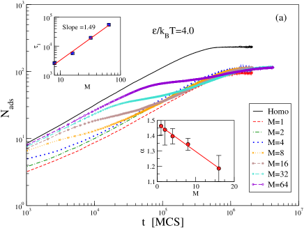
The characteristic shoulder in the adsorption transients of regular multiblock copolymers manifests itself in the early stage of adsorption and lasts progressively longer when $M$ grows. We interpret the temporal length of this shoulder with the time it takes for a segment from the second adsorptive $A$-block in the polymer chain to be eventually captured by the attractive surface, once the first $A$-block has been entirely adsorbed. For sufficiently large blocks one would therefore expect that this time interval, $\tau_{s}$, associated with the capture event, will scale as the Rouse time, $M^{1+2\nu}$, of a non-adsorbing tethered chain of length $M$. The observed $\tau_{s}$ versus $M$ relationship has been shown in the upper left inset in Fig. 6a. The slope of $\approx 1.49$ is less that the Rouse time scaling exponent, $2.18$, which one may attribute to the rather small values of the block length $M$ that were accessible in our simulation. One should also allow for scatter in the end time of the shoulder due to the mismatch in the capture times of all the successive $A$-blocks in the course of our statistical everaging over many chains during the computer experiment.

In the case of random copolymers, Fig. 6b, the observed adsorption transients resemble largely those of a homopolymer chain with the same number of beads again, apart from the expected difference in the plateau height which is determined by the equilibrium number of adsorbed monomers. One should note, however, that a rescaling of the vertical axis with the fraction of sticking monomers, $p$, does not lead to coinciding plateau height - evidently the loops whose size also depends on $p$ also affect the equilibrium number of adsorbed monomers. The variation of the observed scaling exponent $\alpha$ with composition $p$ is shown in the inset to Fig. 6b wherefrom one gets $\alpha\approx 1.6$. Note that this value is considerably lower than the power of $2.24$ which has been observed earlier Shaffer , however, for very short chains with only $10$ sticking beads. One may conclude that even for random copolymer adsorption the typical time of the process scales as $\tau\propto N^{\alpha}$, as observed for homo - and regular block copolymers. It is conceivable, therefore, that an effective zipping mechanism in terms of renormalized segments, that is, segments consisting of an $A$ and $B$ diblock unit of length $2M$ for regular multiblock copolymers provides an adequate notion of the way the adsorption kinetics may be treated even in such more complicated cases. For random copolymers the role of the block length $M$ would then be played by the typical correlation length.

IV.3 Probability Distribution Functions

The time evolution in the corresponding Probability Distribution Functions (PDF) of all the trains, loops and tails of adsorbed polymers provides a lot of information and insight in the kinetics of the adsorption process. In the Appendix we have derived theoretically the expected train distribution under the assumption that local equilibrium of loops of unit length is established much faster than the characteristic time of adsorption itself. The resulting distribution of possible train lengths is shown to be exponential, in close analogy to that of living polymers Greer . In Fig. 7a we plot the observed PDF of train lengths for a chain with $N=256$ at two strengths $\epsilon/k_{B}T$ of the adsorption potential. When scaled with the mean train length $h_{av}(t)=\langle h(t)\rangle$, at time $t$, in both cases for $\epsilon/k_{B}T=3.0\;\mbox{and}\;5.0$ one finds an almost perfect straight line in semi-log coordinates, as predicted by Eq. 32.

Figure 7: (a) Distribution of train lengths during the adsorption process of a homopolymer chain with $N=256$ at two strengths of the adsorption potential $\epsilon$, shown in semi-log coordinates. PDFs for different times (in units of $10^{5}$ MCS) collapse on master curves when rescaled by the mean train length $h_{av}(t)$. (b) Distribution of loop lengths $W(k,t)$ for $N=256$ and $\epsilon/k_{B}T=4.0$ during ongoing polymer adsorption. In the inset the PDF is normalized by $n(t)$ and shown to be a straight line in log-log coordinates.

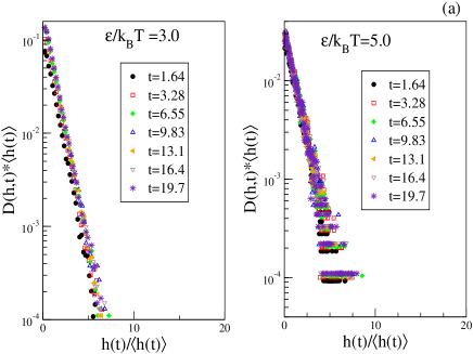
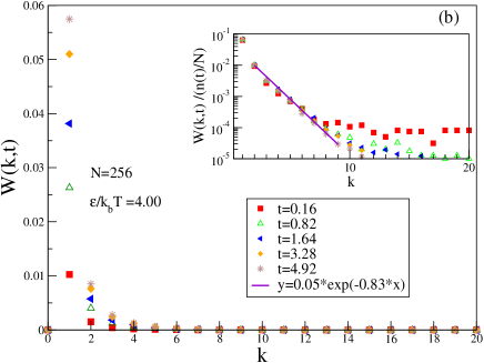
One may thus conclude that the PDF for train lengths preserves its exponential form during the course of the adsorption process, validating thus the conjecture of rapid local equilibrium. The latter, however, is somewhat violated for the case of rather strong adsorption - $\epsilon/k_{B}T=5.0$ - shown in Fig. 7a which is manifested by the increased scatter of data at late times when the adsorption process overtakes to some extent the relaxation kinetics on the surface. The PDF of loops $W(k,t)$ at different times after the onset of adsorption is shown in Fig. 7b. Evidently, the distribution is sharply peaked at size one whereas less than the remaining $20\%$ of the loops are of size two. Thus the loops can be viewed as single thermally activated defects (vacancies) consisting of a desorbed single bead with both of its nearest neighbors still attached to the adsorption plane. As the inset in Fig. 7b indicates, the PDF of loops is also described by an exponential function. The PDFs for loops at different time collapse on a master curve, if scaled appropriately with the instantaneous order parameter $n(t)/N$.

Figure 8: (a) Distribution of tail size for different times (in units of $10^{5}$ MCS) during the polymer chain adsorption for a chain with $N=256$ at $\epsilon/k_{B}T=4.0$. (b) The same as in (a) as derived from the solution of the ME for chain length $N=32$. For better visibility the time slices for $t=1,\;5,\;30\;100,\;150,\;200,\;\mbox{and}\;300$ are shifted along the time axis and arranged such that the initial distribution for $t=1$ is represented by the most distant slice.

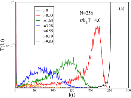
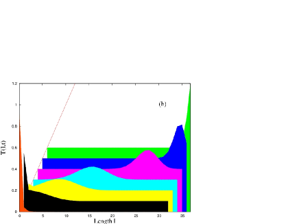
Eventually, in Fig. 8a we present the observed PDF of tails for different times $t$ after the start of adsorption, and compare the simulation results with those from the numeric solution for $T(l,t)$ according to Eq. 10. One may readily verify from Fig. 8 that the similarity between simulational and theoretic results is really strong. In both cases one starts at $t=1$ with a strongly peaked PDF at the full tail length $l(t=1)=N$. As time goes by, the distribution becomes broader and its maximum shifts to smaller values. At late times the moving peak shrinks again and the tail either vanishes, or reduces to a size of single segment which is expressed by the sharp peak at the origin of the abscissa.

V Conclusions

In this study we examine the adsorption kinetics of a single polymer chain on a flat structureless plane in the strong physisorption regime. Adopting the stem-flower model for a chain conformation during adsorption, and assuming the segment attachment process to follow a “zipping” mechanism, we develop a scaling theory which describes the time evolution of the fraction of adsorbed monomers for polymer chains of arbitrary length $N$ at adsorption strength of the surface $\epsilon/k_{B}T$.

We derive a Master Equation as well as the corresponding Fokker-Planck equation for the time-dependent PDF of the number of adsorbed monomers and for the complementary PDF of tails, and define the appropriate reflecting boundary conditions. Inherent in this derivation is the assumed condition of detailed balance which makes it possible to relate the elementary steps of adsorption/desorption. From the numeric solution of the equivalent discrete set of coupled first-order differential equations we find that the growth of the adsorbed fraction of monomers with time is governed by a power law, $n(t)\propto t^{\frac{1}{1+\nu}}$, while the typical time of adsorption $\tau$ scales with the length of the polymer $N$ as $\tau\propto N^{\alpha}$ with $\alpha=1+\nu$. The adsorption transients, found in the Monte Carlo simulation are in good agreement with these predictions, if one takes into account the finite-size effects due to the finite length of the studied polymer chains.

We demonstrate also that the height of the long time plateau in the adsorption transients is determined by the equilibrium number of vacancies (defects) in the trains of adsorbed monomers. The transients themselves are found to collapse on a single master curve, if time is measured in reduced units which scale with the corresponding driving force for adsorption as determined by the surface potential $\epsilon/k_{B}T$.

A deeper insight into the adsorption kinetics is provided by our detailed study of the relevant probability distributions of trains, loops and tails during the adsorption. The predicted exponential expression for the PDF of trains is in a very good agreement with our simulational findings. The loops in the strong physisorption regime are observed to reduce to occasional desorbed segments (vacancies) which play little role in the dominating picture of trains and tails. The PDFs of the latter are found from the simulation data to present a shape which is fully consistent with that of the theoretic treatment. It should be noted also that for chemisorption, a monomer adsorption event involves a significant local activation barrier O'Shaughnessy_1 ; O'Shaughnessy_2 . In this so-called “accelerated zipping“ regime, the loops formation disrupts the adsorption process and the corresponding dynamics differs significantly from the one investigated in this paper.

Eventually, in the case of regular multiblock and random copolymers we find that the adsorption kinetics strongly resembles that of homopolymers. The observed deviations from the latter suggest plausible interpretations in terms of polymer dynamics, however, it is clear that additional investigations will be warranted before a complete picture of the adsorption kinetics in this case is established too.

VI Acknowledgments

We thank J.-U. Sommer for careful reading of the manuscript and helpful discussion. A. Milchev and A. Grosberg are indebted to the Max-Planck Institute for Polymer Research in Mainz, Germany, for hospitality during their visit in the institute. A. Grosberg acknowledges support from the Humboldt Foundation. A. Milchev and V. Rostiashvili gratefully acknowledge support from the Deutsche Forschungsgemeinschaft (DFG), grant No. SFB 625/B4.

Appendix A Derivation of train distribution

The partition function of an one-dimensional array of $p+1$ trains, separated by $p$ defects, has the following form

$$\Phi[n(t),p] = \mathop{\int\dots\int}\limits_{0<x_{1}<x_{2}\dots x_{p}<n(t)}dx_{1}\dots dx_{p}$$ (35)

$$= \int\limits_{0}^{n(t)}\>dx_{1}\int\limits_{x_{1}}^{n(t)}\>dx_{2}\dots\int\limits_{x_{p-1}}^{n(t)}\>dx_{p}=\frac{1}{p!}\>\left[n(t)\right]^{p}$$

where $n(t)$ is the total number of adsorbed monomers at time $t$.

Consider now the the distribution of an arbitrary train $h_{s+1}=x_{s+1}-x_{s}$. In order to find it, one should carry out the integration in Eq. (35) over all $x$-coordinates except $x_{s}$ and $x_{s+1}$. In result of the integration one gets

$$\Phi_{x_{s}x_{s+1}}[n(t),p]\>dx_{s}dx_{s+1}=\frac{1}{(s-1)!(p-s-1)!}\>x_{s}^{s-1}\>\left[n(t)-x_{s+1}\right]^{p-s-1}\>dx_{s}dx_{s+1}$$ (36)

where Eq.(35) has been used separately for the intervals $[0,x_{s}]$ and $[x_{s+1},n(t)]$.

The distribution of the train length, $h_{s+1}=x_{s+1}-x_{s}$, follows immediately from Eq.(36) after integrating over $x_{s}$, i.e.

$$\Phi_{h_{s+1}}[n(t),p]=\frac{1}{(s-1)!(p-s-1)!}\>\>\int\limits_{0}^{n(t)-h_{s+1}}\>x_{s}^{s-1}\>\left[n(t)-h_{s+1}-x_{s}\right]^{p-s-1}\>dx_{s}$$ (37)

By the substitution, $y=x_{s}/[n(t)-h_{s+1}]$, in the integral of eq.(37) one arrives at the result

$$\Phi_{h_{s+1}}[n(t),p] = \frac{\left[n(t)-h_{s+1}\right]^{p-1}}{(s-1)!(p-s-1)!}\>\>\int\limits_{0}^{1}y^{s-1}(1-y)^{p-s-1}\>dy$$ (38)

$$= \frac{1}{(p-1)!}\>\left[n(t)-h_{s+1}\right]^{p-1}$$

where one has used $\int_{0}^{1}y^{s-1}(1-y)^{p-s-1}dy=(s-1)!(p-s-1)!/(p-1)!$. The result in Eq. (38) does not depend on the consecutive number of the train, as expected. The normalized probability to find a train of the length $h$ at time $t$ is given by

$$D(h,t) = \frac{\Phi_{h}[n(t),p]}{\Phi[n(t),p]}=\frac{p!}{(p-1)!}\>\frac{\left[n(t)-h\right]^{p-1}}{\left[n(t)\right]^{p}}$$ (39)

$$= \frac{p}{n(t)}\>\left[1-\frac{h}{n(t)}\right]^{p-1}\simeq\frac{p}{n(t)}\>\exp\left[-h\frac{p}{n(t)}\right]$$

where one uses Eqs.(35) and (38) as well as the conditions $p\gg 1$ and $h/n(t)\ll 1$. Taking into account that the average train length $h_{\rm av}(t)=n(t)/p$, the last expression results in Eq.(32).

References

- (1) G.J. Fleer, M.A. Cohen - Stuart, J.M.H.M. Scheutjens, T. Gosgrove, B. Vincent, Polymers at Interface, Chapman Hall, London, 1993
- (2) P.G. de Gennes, J. Phys (Paris),37, 1445 (1976).
- (3) P.G. de Gennes, Macromolecules 14, 1637 (1981).
- (4) P.G. de Gennes,Macromolecules, 13, 1069 (1980).
- (5) P.G. de Gennes, P. Pincus, J. Phys. (Paris), 44, L-241 (1983).
- (6) P.G. de Gennes, Adv. Colloid Interface Sci. 27, 189 (1987).
- (7) E. Eisenriegler, K. Kremer, K. Binder, J. Chem. Phys. 77, 6296 (1982).
- (8) R. Descas, J.- U. Sommer, A. Blumen, J. Chem. Phys. 120, 8831 (2004).
- (9) S. Metzger, M. Müller, K. Binder, J. Baschnagel, Macromol. Theory Simul. 11, 985 (2002).
- (10) A. Milchev, K. Binder, Macromolecules 29, 343 (1996).
- (11) A. Takahashi, M. Kawaguchi, Adv. Polym. Sci. 46, 1 (1982).
- (12) M. Cohen - Stuart, T. Cosgrove, B. Vinsent, Adv. Colloid Interface Sci. 24, 143 (1986).
- (13) K. Konstadinidis, S. Prager, M. Tirrell, J. Chem. Phys. 97, 7777 (1992).
- (14) J.S. Shaffer, Macromolecules, 27, 2987 (1994).
- (15) P.-Y. Lai, Macromol. Theory Simul. 5, 255 (1996).
- (16) A.L. Ponomarev, T.D. Sewell, C.J. Durning, Macromolecules, 33, 2662 (2000).
- (17) B. O’Shaughnessy, D. Vavilonis, Eur. Phys. J. E 11, 213 (2003).
- (18) B. O’Shaughnessy, D. Vavilonis, J. Phys.: Condens. Matter 17, R63 (2003).
- (19) N.G. van Kampen, Stochastic Processes in Physics and Chemistry, North - Holland, Amsterdam, 1992.
- (20) R. Descas, J.- U. Sommer, A. Blumen, J. Chem. Phys. 124, 094701 (2006).
- (21) F. Brochard-Wyart, Europhys. Lett. 30, 387 (1995).
- (22) T. Sakaure, Phys. Rev.E 76, 021803 (2007).
- (23) C. Vanderzande, Lattice Models of Polymers, Cambridge University Press, cambridge, 1998.
- (24) S. C. Greer, Annu. Rev. Phys. Chem. 53, 173 (2002).
- (25) A. Milchev, K. Binder, Macromolecules, 29, 343 (1996).