Component separation with flexible models.
Application to the separation of astrophysical emissions

Abstract

This paper offers a new point of view on component separation, based on a model of additive components which enjoys a much greater flexibility than more traditional linear component models. This flexibility is needed to process the complex full-sky observations expected from the Planck space mission, for which it was developed, but it may also be useful in any context where accurate component separation is needed.

1 Introduction

This paper describes an advanced component separation technique and its application to the analysis of multi-spectral observations of the Cosmic Microwave Background (CMB). It is developed more specifically in view of the data processing pipeline for the forthcoming Planck mission [1] of the European Spatial Agency (ESA).

Component separation is a critical part of CMB data processing because no frequency channel exists that would be sensitive only to CMB emission. As an illustration, figure 1 shows (simulated) maps of the microwave emission of the sky observed in the frequency channels of Planck i.e. in spectral bands centered around frequencies $\nu=30,44,70,100,143,217,353,545,857~{}\mathrm{GHz}$. The red (in an arbitrary color map) horizontal strips along the Galactic equator, in the middle of the maps, are due to Galactic emissions (that is, emissions from our Galaxy). In contrast, towards the poles where the Galactic emissions are weaker, one can see in the center channels (100, 143 and 217 GHz), an homogeneous texture which is the signal of interest: the (spatial) fluctuations (or ‘anisotropies’) of the CMB. Unfortunately, even in the polar areas, the contamination of the CMB by various astrophysical emissions (or ’foregrounds’, as opposed to the cosmic background) is still significant. There, especially at the smallest angular scales, contamination is dominated by the emission of remote extragalactic objects – galaxies (or ‘point sources’) of various types (which emit radiation through similar physical processes as our own Galaxy), and galaxy clusters (which emit via the Sunyaev-Zel’dovich effect, hereafter: the ‘SZ component’).

There is no significant occlusion between the various physical components so that the signal $X_{\nu}(\xi)$ measured at a frequency $\nu$ in direction $\xi$ is a linear superposition:

$$X_{\nu}(\xi)=X_{\nu}^{\mathrm{cmb}}(\xi)+X_{\nu}^{\mathrm{gal}}(\xi)+X_{\nu}^{\mathrm{SZ}}(\xi)+\ldots+N_{\nu}(\xi)$$

where $X_{\nu}^{\mathrm{x}}(\xi)$ is the contribution due to a particular component $\mathrm{x}$ and $N_{\nu}(\xi)$ accounts for instrumental noise at the map level.

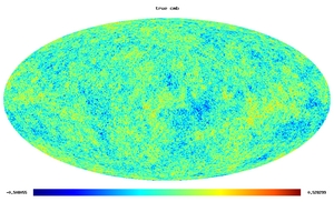
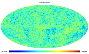
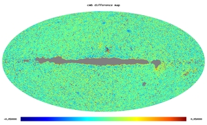
It must be stressed that, even though the lowest (30, 44, 70 GHz) and highest (353, 545, 857 GHz) frequency channels are more contaminated by Galactic emissions, they still are very informative because they can be used to predict and remove the Galactic emission in the center channels, leaving only CMB and noise… in an ideal data processing scenario. Successful scientific exploitation of the CMB measurements for cosmological studies critically depends on accurate cleaning of the CMB and on quantifying as well as possible any remaining contamination. Figure 8 illustrates on simulated data what can be achieved with our technique on a very large fraction of the sky.

Even though CMB recovery is the main goal, recovering the other components also is of scientific interest. For instance, Planck should also yield a very rich catalog of galaxy clusters, and provide a lot of information about the emission of the interstellar medium in our own Galaxy. Hence, we are actually facing a problem of component separation from multiple observations.

The component separation problem is not new to the astrophysics community. In the past ten years however, component separation for CMB observations specifically has motivated the development of a large variety of methods with various degrees of sophistication (see [7] for a review). The most direct methods rely on modelling and subtracting foreground emission. Such methods, typically, involve a thorough understanding of the emission processes, necessary to build the foreground model. Other methods use simple decorrelation, or make use of differences between properly weighted maps [11]. The processing of data from the WMAP satellite mission makes uses of both kinds of methods [2].

The large majority of existing component separation methods in the context of CMB observations rely on a ‘mixing model’ as follows: for any available direction $\xi$ in the sky, the $m$ channels at frequencies $\nu_{1},\ldots,\nu_{m}$ provide $m$ data points which can be collected in an $m\times 1$ vector $X(\xi)$ which is modelled as

$$X(\xi)=\mathbf{A}S(\xi)+N(\xi)$$ (1)

where each entry of $S(\xi)$ contains the sky-pattern for the emission of a given component. The emissivity of a given component depends on the frequency $\nu$; hence, each column of matrix $\mathbf{A}$ reflects the emission law of the corresponding component. This equation, then, forms the basis for many component separation algorithms but it forces a special structure on each component, namely that it ‘scales rigidly with frequency’. Some methods are developed to solve this component separation problem when the mixing matrix $A$ is known a priori. This is the case, for instance, of the work described in [20, 12, 4, 19].

Component separation is a well studied problem in Signal Processing, but the nature of the available data and the scientific objectives call for specific techniques. In particular, one may think of resorting to Independent Component Analysis (ICA) methods since these ‘blind’ techniques may be useful to deal with some of the uncertainties in the data structure. In addition, columns of the mixing matrix $\mathbf{A}$ corresponding to some of the astrophysical components (e.g. components modelling the emission of our own Galaxy) are known a priori up to significant uncertainty, and more precise knowledge is an objective of the forementioned astrophysical observations. Implementations of ICA ideas in the context of CMB observations can be found in [13, 18, 6, 14, 3].

Compared with all the above methods, our framework allows the inclusion of components with arbitrary structure (at least in terms of second order correlations). This structure, as will be detailed later on, can be matched to prior knowledge of the nature of the astrophysical emission. Along the same spirit of matching a parametric model of the emissions to the data, although quite different in implementation, are the work described in [21, 9].

Although there is substantial motivation for letting the data alone indicate the appropriate model of the emissions, a fully blind approach would leave out a lot of valuable prior information in the CMB context. The approach described in this paper is rooted in ICA but allows for the inclusion an arbitrary amount of prior information, in particular by allowing components with an arbitrary structure.

Again, the approach to component separation described herein is not specific to this particular problem and may be considered for application to any situation where ‘expensive’ data deserve special care and have to be fitted by a complex component model.

The paper is organized as follows: section 2 describes our approach, section 3 focuses in specific aspects; implementation is discussed in section 4 in terms of a library of components; section 5 illustrates an application of the method on data from the Planck sky model.

2 A flexible approach to component separation

This section introduces a key ingredient of our approach: the development of a flexible model of additive components in which the notion of ‘mixing matrix’, which is central to standard ICA, is disposed of. Not only the mixing matrix is not needed but it is ‘considered harmful’.

2.1 Unconstrained components

We start the exposition by considering the most general component model for an $m\times 1$ random vector $X$: we only postulate that $X$ is made of the linear superposition of $C$ components:

$$X=\sum_{c=1}^{C}X^{c}$$ (2)

where each component $X^{c}$ is an $m\times 1$ random vector. For simplicity, we shall assume that all components have zero mean. Denote $\mathbf{R}$ (resp. $\mathbf{R}^{c}$) the covariance matrix of vector $X$ (resp. of its $c$-th component $X^{c}$). A key assumption of our model is mutual decorrelation between all components, which implies that the covariance matrix of $X$ decomposes as

$$\mathbf{R}=\sum_{c=1}^{C}\mathbf{R}^{c}.$$ (3)

Consider now recovering linearly a particular component $X^{c}$ from the superposition (2). Denote $\mathbf{W}_{c}$ the $m\times m$ matrix which best predicts $X^{c}$ based on $X$ in the sense that

$$\mathbf{W}_{c}=\arg\min_{\mathbf{W}}\operatorname{E}|\mathbf{W}X-X^{c}|^{2}.$$ (4)

this problem is easily solved under our assumptions and one readily finds:

$$\mathbf{W}_{c}=\mathbf{R}^{c}\mathbf{R}^{-1}$$ (5)

At this stage, we wish to deliver a simple but important message: eq. (5) means that component separation, understood as computing $\widehat{X}^{c}=\mathbf{W}^{c}X$, requires only knowing $\mathbf{R}^{c}$ and $\mathbf{R}$. Of course, covariance matrix $\mathbf{R}$ may (but need not to) be simply estimated from the empirical covariance matrix $\widehat{\mathbf{R}}$ of $X$. Therefore, component separation is solved if we can uniquely solve the covariance separation problem, in the sense of identifying the component terms $\mathbf{R}^{c}$ in decomposition (3).

In order to achieve covariance separation, some additional information or assumptions are of course needed. Our method jointly exploits two possibilities: considering localized matrices (for more information) and considering structured matrices (for more constraints).

2.2 Localized statistics, localized separation

This section defines the ‘localized statistics’ on which our method is based. Consider the component separation problem based on $p$ samples on $m$ detectors. We shall not compress this data set into a single sample $m\times m$ covariance matrix but rather ‘localize’ the statistics and form a set of localized covariance matrices. By ‘localization’, we typically mean localization in time, space, frequency, wavelet space, depending on the problem at hand. The simplest example of localization is suggested by the separation of non-stationary time series as considered in [15, 16] where the data are time-indexed and one would divide the observation interval into $Q$ sub-intervals and compute an estimate of the covariance of $X$ over each of these intervals.

More generally, we assume that the data are available as $p$ vectors $X(1),\ldots,X(p)$, each of size $m\times 1$ where the $i$-th entry of $X(j)$ is either the $j$-th sample of the $i$-th input signal or its $j$-th coefficient in some basis (e.g. the Fourier basis). In our application to CMB analysis, we use the spherical harmonic basis (see section 5). Basis choice is discussed below; it does have an impact on separation but it does not change the nature of the problem in the sense that, if the component model (2) holds in some basis, it also holds in any other basis and that if a component is reconstructed in a given basis, it becomes available in any basis.

Localized statistics are formed by dividing the index set $[1,\ldots,p]$ into $Q$ subsets which are called ‘domains’ in the following (time domains would be time intervals, spectral domains would be frequency bands, etc…). Denoting $\mathcal{D}_{q}$ the $q$-th domain, partitioning of the data set reads $[1,\ldots,p]=\cup_{q=1}^{Q}\mathcal{D}_{q}$ and localized statistics are computed (defined) as

$$\widehat{\mathcal{R}}=\{\widehat{\mathbf{R}}_{q}\}_{q=1}^{Q},\qquad\widehat{\mathbf{R}}_{q}=\frac{1}{p_{q}}\sum_{j\in\mathcal{D}_{q}}X(j)X(j)^{\dagger},$$ (6)

where $p_{q}$ is the number of coefficients in domain $\mathcal{D}_{q}$.

The expected value of the sample covariance matrix for the $q$th domain is defined/denoted as

$$\mathbf{R}_{q}=\operatorname{E}\widehat{\mathbf{R}}_{q}$$

and we shall use the same notation for each component so that, these being mutually uncorrelated by assumption, one has the decomposition

$$\mathbf{R}_{q}=\sum_{c=1}^{C}\mathbf{R}_{q}^{c}\qquad\mathbf{R}_{q}^{c}=\operatorname{E}\Bigl{\{}\frac{1}{p_{q}}\sum_{j\in\mathcal{D}_{q}}X^{c}(j)X^{c}(j)^{\dagger}\Bigr{\}}=\frac{1}{p_{q}}\sum_{j\in\mathcal{D}_{q}}\operatorname{Cov}X^{c}(j)$$ (7)

We can then perform a localized separation in the sense that the localized Wiener filter for recovering component $c$ in domain $q$ is

$$\widehat{X}^{c}(j)=\mathbf{R}_{q}^{c}\mathbf{R}_{q}^{-1}X(j)\ \ \text{for}\ \ j\in\mathcal{D}_{q}$$ (8)

A key point is that, by definition, this filter is specialized to operate on domain $q$, hence it is adapted to the local correlation conditions.

2.3 Constrained components and model identification

Implementing component separation by (8) requires knowning the local covariance matrices $\mathbf{R}_{q}^{c}$. These are usually unknown and must be estimated, based on $\widehat{\mathbf{R}}_{q}$, the sample estimate (6) of their sum. It goes without saying that, without constraining the possible values of $\mathbf{R}_{q}^{c}$, it is not possible in general to uniquely resolve (an estimate of) this sum into its components. Constraining a given component $c$ is achieved by parametrizing the matrix set $\mathcal{R}^{c}=\{\mathbf{R}_{q}^{c}\}_{q=1}^{Q}$ by a parameter vector $\theta^{c}$ i.e. a parametric model for the $c$-th component is a function $\theta^{c}\rightarrow\mathcal{R}^{c}(\theta^{c})=\{\mathbf{R}_{q}^{c}(\theta^{c})\}_{q=1}^{Q}$. Some examples of these parametric models are given in section 3.2.

A parametric model $\theta\rightarrow\mathcal{R}(\theta)$ follows by assuming component decorrelation (7) and taking the global parameter $\theta$ as the concatenation of the parameter vectors of each component:

$$\mathcal{R}(\theta)=\{\mathbf{R}_{q}(\theta)\}_{q=1}^{Q}=\bigl{\{}\sum_{c}\mathbf{R}_{q}^{c}(\theta^{c})\bigr{\}}_{q=1}^{Q}\qquad\theta=(\theta^{1},\ldots,\theta^{c}).$$

The parametric model is identified by fitting it to data, that is, by minimizing a measure of mismatch between $\widehat{\mathcal{R}}$ and $\mathcal{R}(\theta)$ as:

$$\widehat{\theta}=\arg\min\phi(\theta)\quad\text{where}\quad\phi(\theta)=\sum_{q=1}^{Q}w_{q}K(\widehat{\mathbf{R}}_{q},\mathbf{R}_{q}(\theta))$$ (9)

where $K(\cdot,\cdot)$ is measure of mismatch between two positive $m\times m$ matrices and $w_{q}$ are positive weights. Our most common choice is to use

$$w_{q}=p_{q}\quad\text{and}\quad K(\mathbf{R}_{1},\mathbf{R}_{2})=\frac{1}{2}\left[\mathrm{trace}(\mathbf{R}_{1}^{-1}\mathbf{R}_{2})-\log\det(\mathbf{R}_{1}^{-1}\mathbf{R}_{2})-m\right]$$ (10)

because this is the form which stems from the maximum likelihood principle. Specifically, if a coefficient $X(i)$ belonging to domain $q$ is modeled as $X(i)\sim\mathcal{N}(0,\mathbf{R}_{q})$ and as independent from $X(i^{\prime})$ for $i\neq i^{\prime}$, then $\phi(\theta)$ is the negative log-likelihood of the model [16].

2.4 Summary

In summary, our method is based on the following steps and design choices:

1. Choice of a basis to obtain coefficients $X(i)$ (original space, Fourier or spherical-harmonic space, wavelet space,…).

2. Choice of domains $\{\mathcal{D}_{q}\}_{q=1}^{Q}$ to localize their second-order statistics $\widehat{\mathcal{R}}$,

3. Choice of a model $\theta^{c}\rightarrow\mathcal{R}^{c}(\theta^{c})$, for the contribution $\mathbf{R}_{q}^{c}$ of each component $c$ to the covariance matrix over each domain $q$.

4. Minimization of the matching criterion (9) to obtain the estimate $\hat{\theta}$, hence estimates $\hat{\theta}^{c}$ for the parameters of each component.

5. Estimation of the coefficients of each component by $\widehat{X}^{c}(j)=\mathbf{R}_{q}^{c}(\hat{\theta}^{c})\mathbf{R}_{q}(\hat{\theta})^{-1}X(j)$, that is the version of (8) based on estimated parameters.

6. Reconstruction of the components from their coefficients $\widehat{X}^{c}(j)$.

At this stage, most of the statistical framework is in place but our method is not completely specified yet because of the flexibility in design choices in items 1, 2 and 3 above among other issues. Next section discusses some of them.

3 Discussion

3.1 Correlated or multi-dimensional components

We wish to contrast the standard form $X=\mathbf{A}S+N$ of the noisy linear component model of eq. (1) with the unconstrained model $X=\sum_{c}X^{c}$ of eq. (2). Obviously, the standard model is included in the unconstrained model since one may always write $\mathbf{A}S+N=\sum_{c=1}^{C}X^{c}$ with $X^{c}=\mathbf{a}_{c}S_{c}$ for $1\leq c\leq n$ and $X^{C}=X^{n+1}=N$ where $\mathbf{a}_{c}$ denotes the $c$-th column of $\mathbf{A}$ and $S_{c}$ denotes the $c$th entry of $S$.

A component $X^{c}(\xi)$ which can be written as $X^{c}(\xi)=\mathbf{a}_{c}S_{c}(\xi)$ is fully coherent in the sense that any two entries of vector $X^{c}(\xi)$ are 100% correlated. Of course, this is because all the randomness in $X^{c}(\xi)=\mathbf{a}_{c}S_{c}(\xi)$ comes from a single scalar random variable $S_{c}(\xi)$. A fully coherent component contributes exactly the same pattern on all sensors (or channels) up to a fixed proportionality coefficient. It has a rank-one covariance matrix: $\mathbf{R}^{c}=\operatorname{Cov}(S_{c}(\xi))\mathbf{a}_{c}\mathbf{a}_{c}^{\dagger}$; for this reason, it could also be called a one-dimensional since it leaves in the 1D space spanned by vector $\mathbf{a}_{c}$ or in the 1D range space of $\mathbf{R}^{c}$.

In our application, the CMB is a fully coherent component: from one frequency channel to another, only its overall intensity changes (ignoring the frequency-dependent resolution). This is in contrast with, for instance, the Galactic emission, which cannot be represented over the sky as a fully coherent component (see fig. 2).

Assume now that, in the model $X=\mathbf{A}S+N$, two sources, say $i$ and $j$, are statistically dependent while all other pairs of sources in $S$ are mutually independent. These two sources contribute $\mathbf{a}_{i}S_{i}+\mathbf{a}_{j}S_{j}$ to $X$ and we decide to lump them into a single component denoted $X^{c}$ for some index $c$: $X^{c}=\mathbf{a}_{i}S_{i}+\mathbf{a}_{j}S_{j}$. Then $X$ can still be written as in eq. (2) and all the components $X^{c}$ are independent, again. In other words, we represent here the contributions of two correlated sources as the contribution of a single 2-dimensional component: we now have one less component but it is 2-dimensional. Clearly, this component is not fully coherent: it contributes a pattern on sensor $m$ which is not proportional to the pattern contributed to another sensor $m^{\prime}$. One can obviously define multidimensional components of any dimension, each one possible representing the contribution of several correlated sources. In section 5, we use a 4-dimensional component to model Galactic emission.

Note that, in eq. (2), the noise term is included as one of the components. If the noise is uncorrelated from channel to channel, as is often the case, then the noise component is $m$-dimensional (the largest possible dimension).

More generally, our model does not require any component to be low dimensional. Rather, our model is a plain superposition of $C$ components as in eq. (2). None of these components is required to have any special structure, one-dimensional or otherwise.

3.2 Library of components

We call a collection of parametric models $\theta^{c}\rightarrow\mathcal{R}^{c}(\theta^{c})$ a library of components. In practice, each member of the library must not only specify a parametrization $\theta^{c}\rightarrow\mathcal{R}^{c}(\theta^{c})$ but also its gradient and related quantities (see sec. 4.2).

Typical examples of component models are now listed.

1. The ‘classic’ ICA component is fully coherent (one dimensional) $X^{c}(i)=\mathbf{a}_{c}S_{c}(i)$. Denoting $\sigma_{qc}^{2}$ the average variance of $S_{c}(i)$ over the $q$th domain, the contribution $\mathbf{R}_{q}^{c}$ of this component to $\mathbf{R}_{q}$ is the rank-one matrix

   $$\mathbf{R}_{q}^{c}=\mathbf{a}_{c}\mathbf{a}_{c}^{\dagger}\sigma_{qc}^{2}$$

   This component can be described by an $(m+Q)\times 1$ vector $\theta^{c}$ of parameters containing the $m$ entries of $\mathbf{a}_{c}$ and the $Q$ variance values $\sigma_{qc}^{2}$. Such a parametrization is redundant, but we leave this issue aside for the moment.

2. A $d$-dimensional component can be modeled as

   $$\mathbf{R}_{q}^{c}=\mathbf{A}_{c}P_{qc}\mathbf{A}_{c}^{\dagger}$$

   where $\mathbf{A}_{c}$ is an $m\times d$ matrix and $P_{qc}$ is an $d\times d$ positive matrix varying freely over all domains. This can be parametrized by a vector $\theta^{c}$ of $m\times d+Q\times d(d+1)/2$ scalar parameters (the entries of $\mathbf{A}_{c}$ and of $P_{qc}$). Again, this is redundant, but we ignore this issue for the time being.

3. Noise component. A simple noise model is given by

   $$\mathbf{R}_{q}^{c}=\mathrm{diag}(\sigma_{1}^{2},\ldots,\sigma_{m}^{2})$$

   that is, uncorrelated noise from channel to channel, with the same level in all domains but not in all channels. This component is described by a vector $\theta^{c}$ of only $m$ parameters. A more general model is $\mathbf{R}_{q}^{c}=\mathrm{diag}(\sigma_{1q}^{2},\ldots,\sigma_{mq}^{2})$ meaning that the noise changes from domain to domain; then parameter vector $\theta^{c}$ has size $mQ\times 1$.

4. As a final example, for modeling ‘point sources’ in spectral domain, one may use $\mathbf{R}_{q}^{c}=\mathbf{R}_{\star}^{c}$. Such a component contributes identically in all domains corresponding to a flat spectrum. If, for instance, we assume that this contribution $\mathbf{R}_{\star}^{c}$ is known, then the parameter vector $\theta^{c}$ is void. If $\mathbf{R}_{\star}^{c}$ is known up to a scale factor, then $\theta^{c}$ is just a scalar, etc…In the demonstration test discussed in 5, however, we consider instead the sum of Galactic and point source emission as one single 4-dimensional component – a choice which the flexibility of the present model allows us to do.

3.3 About localization

There are two strong, very different motivations for localizing the statistics.

Localization for accuracy. The first motivation is separation accuracy. If the strength of the various components (including noise) varies significantly across the domains $\mathcal{D}_{q}$, reconstruction is improved by the localized filter. Indeed, the best linear reconstruction of $X^{c}(j)$ based on $X(j)$ would be, as seen above, obtained as $\widehat{X}^{c}(j)=\operatorname{Cov}(X^{c}(j))\operatorname{Cov}(X(j))^{-1}X(j)$. This requires knowing both $\operatorname{Cov}(X^{c}(j))$ and $\operatorname{Cov}(X(j))$. In practice, it seems difficult to obtain estimates for these matrices for all samples, i.e. for each value of $j$. However, if they do not vary too much for all values of $j$ across a domain $\mathcal{D}_{q}$, then a good approximation to the best reconstruction is (8) i.e. the reconstruction filter also is localized, taking advantage of the ‘local SNR conditions’ on domain $\mathcal{D}_{q}$.

Localization for diversity/identifiability. Second, the diversity of the statistics of the components over several domains is precisely what may make this model blindly identifiable. For instance, in the basic ICA model (all components are one-dimensional, no noise), if $X(i)$ are Fourier coefficients and $\mathcal{D}_{q}$ are spectral bands, it is known that spectral diversity (no two components have identical spectrum) is a sufficient condition for blind identifiability.

3.4 About blindness and the Fisher information matrix

Is this a blind component separation method? It all depends on the component model. If all components are modeled as ‘classic’ ICA components (see Sec. 3.2), then the method is as blind as regular ICA. Our approach, however, leaves open the possibility of tuning the blindness level at will by specifying more or less stringent models $\theta^{c}\rightarrow\mathcal{R}^{c}$ for some or all of the components.

Of course, it may be difficult to predict if a given parametrization ensures the identifiability of the model: this is to be discussed on a case-by-case basis. However, over-parametrization can be tested numerically because the Fisher information matrix (FIM) is available in our framework. It has a natural block structure where the block related to a pair $(c,c^{\prime})$ of components is the matrix of size $|\theta^{c}|\times|\theta^{c^{\prime}}|$:

$$[\mathbf{F}(\theta)]_{cc^{\prime}}=\frac{1}{2}\sum_{q}p_{q}\ \mathrm{trace}\left(\frac{\partial\mathbf{R}_{q}^{c}(\theta^{c})}{\partial\theta^{c}}\mathbf{R}_{q}^{-1}(\theta)\frac{\partial\mathbf{R}_{q}^{c^{\prime}}(\theta^{c^{\prime}})}{\partial\theta^{c^{\prime}}}\mathbf{R}_{q}^{-1}(\theta)\right)$$ (11)

under the assumptions which make the mismatch measure $\phi(\theta)$ proportional to the log-likelihood (see sec. 2.3). The FIM is also used for computing (approximate) error bars.

4 Implementation

We discuss the practical issue of actually minimizing the mismatch $\phi(\theta)$ using an arbitrary library of components.

Note that for a noise-free model containing only ‘classic ICA’ components (no other constraints than being one-dimensional), criterion $\phi(\theta)$ boils down to a joint diagonalization criterion which can be very efficiently minimized by a specialized algorithm [17]. For a model including only unconstrained multi-dimensional components and noise, it is possible to use the EM algorithm [6]. EM, however, is not convenient for general component models and, in addition, it appears too slow for our purposes. Therefore, we had to consider more efficient and more general optimization procedures.

4.1 Optimization

We found the Conjugate Gradient (CG) algorithm well suited for minimizing $\phi(\theta)$. Its implementation requires computing the gradient $\partial\phi/\partial\theta$ and (possibly an approximation of) the Hessian $\partial^{2}\phi/\partial\theta^{2}$ for pre-conditioning. Since $\phi(\theta)$ actually is a negative log-likelihood in disguise, its Hessian can classically be approximated by $\mathbf{F}(\theta)$, the Fisher information matrix (FIM) of eq. (11). These computations offer no particular difficulty in theory but we aim at an implementation it in the framework of a library of components i.e. computations should be organized in such a way that each component model $\mathcal{R}_{c}(\theta^{c})$ works as a ‘plug-in’.

4.2 Computing derivatives

Computing the gradient. The partial derivative of $\phi$ with respect to $\theta^{c}$ takes the form

$$\frac{\partial\phi(\theta)}{\partial\theta^{c}}=\sum_{q=1}^{Q}\mathrm{trace}\left(\mathbf{G}_{q}(\theta)\frac{\partial\mathbf{R}_{q}^{c}(\theta^{c})}{\partial\theta^{c}}\right)$$ (12)

where matrix $\mathbf{G}_{q}(\theta)$ is defined as

$$\mathbf{G}_{q}(\theta)=\frac{1}{2}w_{q}\mathbf{R}_{q}^{-1}(\theta)\left(\mathbf{R}_{q}(\theta)-\widehat{\mathbf{R}}_{q}\right)\mathbf{R}_{q}^{-1}(\theta).$$ (13)

Hence the computation of $\partial\phi/\partial\theta$ at a given point $\theta=(\theta^{1},\ldots,\theta^{C})$ can be organized as follows. A first loop through all components computes $\mathcal{R}(\theta)$ by adding up the contribution $\mathcal{R}^{c}(\theta^{c})$ of each component. Then, a second loop over all $Q$ domains computes matrices $\{\mathbf{G}_{q}(\theta)\}_{q=1}^{Q}$ which are stored in a common work space. Finally, a third loop over all components concatenates all partial gradients $\partial\phi/\partial\theta^{c}$, each component implementing the computation of the right hand side of (12) in the best possible way, using the available matrices $\{\mathbf{G}_{q}(\theta)\}_{q=1}^{Q}$.

Computing an (approximate) Hessian. The Fisher information matrix can be partitioned component-wise and each block be computed according to eq. (11). Therefore its computation can be organized with a double nested loop over $c$ and $c^{\prime}$ as soon as the code implementing a given component is able to return the matrix set $\{\frac{\partial\mathbf{R}_{q}^{c}(\theta^{c})}{\partial\theta^{c}}\}_{q=1}^{Q}$. A straightforward implementation of this idea may be impractical, though, because this is a set of $|\theta^{c}|\times Q$ matrices, possibly very large. This problem can be alleviated in the frequent case where components have ‘local’ variables.

Local variables. Consider the case when $\theta^{c}$ can be partitioned into $Q+1$ blocks: $\theta^{c}=(\theta_{0}^{c},\theta_{1}^{c},\ldots,\theta_{Q}^{c})$ where, for $q>0$, the sub-vector $\theta_{q}^{c}$ affects only $\mathbf{R}_{q}^{c}$ while $\theta_{0}^{c}$ collects all the remaining parameters i.e. those which affect the covariance matrix over two or more domains. We then say that this component model has ‘local variables’. This is a fairly frequent situation which occurs for instance when the power of a component can be freely adjusted in each domain (the simplest example is the ‘classic’ ICA component: $\mathbf{R}_{q}^{c}=\mathbf{a}_{c}\mathbf{a}_{c}^{\dagger}\sigma_{qc}^{2}$, for which $\theta_{0}^{c}=\mathbf{a}$ and $\theta_{q}^{c}=\sigma_{qc}^{2}$ for $q=1,\ldots,Q$. The global parameter vector $\theta$ inherits this structure by being partitioned accordingly into a ‘global part’ $\theta_{0}=(\theta_{0}^{1},\ldots,\theta_{0}^{C})$ and $Q$ local parts $\theta_{q}=(\theta_{q}^{1},\ldots,\theta_{q}^{C})$.

A first and major benefit of such a local/global partitioning is that it introduces many zero blocks in the FIM since then $[\mathbf{F}(\theta)]_{qq^{\prime}}=\mathbf{0}$ for $1\leq q\neq q^{\prime}\leq Q$, allowing the computation of the pre-conditioned gradient $\mathbf{F}(\theta)^{-1}\partial\phi/\partial\theta$ to be organized much more efficiently.

Another benefit of the local/global partitioning is that it makes it easy to implement a ‘local optimization’: during global optimization over $\theta$, it is possible at any time to loop through all $Q$ domains and to solve in each domain, possibly exactly, the sub-problem $\min_{\theta_{q}}K(\widehat{\mathbf{R}}_{q},\mathbf{R}_{q}(\theta_{0},\theta_{q})\,)$ which is, of course, of much smaller size than the original problem in most cases.

4.3 Indeterminations and penalization.

Examples of section 3.2 show that ‘natural’ component parametrizations often are redundant. From a statistical point of view, this is not important: we seek ultimately to identify $\mathcal{R}^{c}=\{\mathbf{R}_{q}^{c}\}_{q=1}^{Q}$ as a member of a family described by a mapping $\theta^{c}\rightarrow\mathcal{R}^{c}(\theta^{c})$ but this mapping does not need to be one-to-one. The simplest example again is for $\mathbf{R}_{q}^{c}=\mathbf{a}_{c}\mathbf{a}_{c}^{\dagger}\sigma_{qc}^{2}$ which is invariant if one changes $\mathbf{a}_{c}$ to $\alpha\mathbf{a}_{c}$ and $\sigma_{qc}$ to $\alpha^{-1}\sigma_{qc}$. Therefore, there is a 1D set of pairs $(\mathbf{a}_{c},\sigma_{qc})$ achieving the global optimum but they all correspond to a unique value of $\mathbf{R}_{q}^{c}$ itself, which is thus perfectly well defined at the optimum and is the unique quantity needed to reconstruct the $c$-th component in domain $q$.

The only serious concern about over-parametrization is from the optimization point of view. Redundancy makes the $\phi(\theta)$ criterion flat in the redundant directions and it makes the FIM a singular matrix. Finding non redundant re-parametrizations is a possibility, but it is often simpler to add a penalty function to $\phi(\theta)$ for any redundantly parametrized component. For instance, the scale indetermination of the classic ICA component $\mathbf{R}_{q}^{c}=\mathbf{a}_{c}\mathbf{a}_{c}^{\dagger}\sigma_{qc}^{2}$ when parametrized $\theta_{0}^{c}=\mathbf{a}_{c}$ and $\theta_{q}^{c}=\sigma_{qc}^{2}$ ($q>1$) is fixed by adding $\phi^{c}(\theta^{c})=g(\|\mathbf{a}_{c}\|^{2})$ to $\phi(\theta)$, where $g(u)$ is any reasonable function which has a single minimum at, say, $u=1$. Of course, the addition such a term should be reflected in the gradient and the Hessian of the matching criterion.

5 Results on simulated Planck data

This section describes an application of our framework to a CMB data set. Although we go into some detail, several issues cannot be discussed due to limited page space. The main objective here is illustrative.

5.1 Data

In preparation for data acquisition by the Planck mission, the ability to perform component separation is evaluated by resorting to a realistic set of simulated data which is developed within the Planck collaboration as the ‘Planck sky model’ (PSM). This suite of programs is used to generate random realizations of the sky at the Planck frequency range compatible with the present knowledge of all identified component emissions and aims at capturing many of the intricacies (both from the sky and from the instrument) expected from real data.

We use sky maps simulated at the 9 frequencies of Planck channels. The instrument point spread function is modelled as a Gaussian beam whose width decreases with increasing frequency: the beams’ FWHM are 33, 24, 14, 10, 7.1, 5, 5, 5, 5 in arcminutes. The beam effect is visible in figure 2 where the angular size of the galaxy clusters (via the SZ effect), point sources and CMB anisotropies decreases from top to bottom reflecting the increasing resolution.

Planck does not take a ‘snapshot’ of the sky. Rather, sky maps are (painfully) computed from sky scans. Due to various technological constraints, the scanning strategy does not guarantee that all pixels are seen (or ‘hit’) equally often. As an important consequence, the variance of the noise in each pixel depends on its hit-count. In our simulated data set, the noise is modelled as Gaussian, independent from channel to channel, from pixel to pixel and with a variance inversely proportional to the hit-count. See fig. 3 for a sky map of hit counts corresponding to a one year survey. The noise variance in one pixel for one hit depend on the frequency channel and are given for the 9 channels by 1027, 1434, 2383, 1245, 753.6, 609.1, 424.5, 154.9, 71.8 $\mu\mathrm{K}^{2}$ for the maps used in this simulation.

The full-sky maps used as inputs to our experiments are shown on figure 1. Figure 2 zooms in and shows the various physical components used as ingredients: CMB, Galactic emissions, galaxy clusters (via the SZ effect), point source emissions (due to infrared- and radio-galaxies). Galactic emission is shown as a single component but is actually made up of three physical components due to free-free, synchrotron and dust emissions.

Figure 1: Simulated full-sky observations at the Planck frequencies: 30, 44, 70, 100, 143, 217, 353, 545, 847 GHz. Color scale: $\pm 0.5$ mKRJ

.

$$\begin{array}[]{c}\includegraphics[width=56.9055pt]{./figs/map--2048-allplanck-030--.jpg}\\ \includegraphics[width=56.9055pt]{./figs/map--2048-allplanck-070--.jpg}\\ \includegraphics[width=56.9055pt]{./figs/map--2048-allplanck-217--.jpg}\\ \includegraphics[width=56.9055pt]{./figs/map--2048-allplanck-857--.jpg}\\ \mbox{\tiny{data}}\end{array}=\begin{array}[]{c}\includegraphics[width=56.9055pt]{./figs/map--2048-cmbplanck-030--.jpg}\\ \includegraphics[width=56.9055pt]{./figs/map--2048-cmbplanck-070--.jpg}\\ \includegraphics[width=56.9055pt]{./figs/map--2048-cmbplanck-217--.jpg}\\ \includegraphics[width=56.9055pt]{./figs/map--2048-cmbplanck-857--.jpg}\\ \mbox{\tiny{CMB}}\end{array}+\begin{array}[]{c}\includegraphics[width=56.9055pt]{./figs/map--2048-galplanck-030--.jpg}\\ \includegraphics[width=56.9055pt]{./figs/map--2048-galplanck-070--.jpg}\\ \includegraphics[width=56.9055pt]{./figs/map--2048-galplanck-217--.jpg}\\ \includegraphics[width=56.9055pt]{./figs/map--2048-galplanck-857--.jpg}\\ \mbox{\tiny{Galactic}}\end{array}+\begin{array}[]{c}\includegraphics[width=56.9055pt]{./figs/map--2048-thermalszplanck-030--.jpg}\\ \includegraphics[width=56.9055pt]{./figs/map--2048-thermalszplanck-070--.jpg}\\ \includegraphics[width=56.9055pt]{./figs/map--2048-thermalszplanck-217--.jpg}\\ \includegraphics[width=56.9055pt]{./figs/map--2048-thermalszplanck-857--.jpg}\\ \mbox{\tiny{SZ}}\end{array}+\begin{array}[]{c}\includegraphics[width=56.9055pt]{./figs/map--2048-poncplanck-030--.jpg}\\ \includegraphics[width=56.9055pt]{./figs/map--2048-poncplanck-070--.jpg}\\ \includegraphics[width=56.9055pt]{./figs/map--2048-poncplanck-217--.jpg}\\ \includegraphics[width=56.9055pt]{./figs/map--2048-poncplanck-857--.jpg}\\ \mbox{\tiny{PS}}\end{array}+\begin{array}[]{c}\includegraphics[width=56.9055pt]{./figs/map--2048-noiseplanck-030--.jpg}\\ \includegraphics[width=56.9055pt]{./figs/map--2048-noiseplanck-070--.jpg}\\ \includegraphics[width=56.9055pt]{./figs/map--2048-noiseplanck-217--.jpg}\\ \includegraphics[width=56.9055pt]{./figs/map--2048-noiseplanck-857--.jpg}\\ \mbox{\tiny{noise}}\end{array}$$

Figure 2: A zoom on a patch of size 17$\times$17 degrees, close to the Galactic plane for the channels at 30, 70, 217 and 857 GHz. The figure shows (in arbitrary color scales) the contributions of each physical component.

Figure 3: Left: Hit-counts map for the 30 GHz channel. In each pixel, noise variance is inversely proportional to it. The number of hits in this map goes from around 40 to 2320.Right: the zones (masks) used in the analysis: polar zone (red), intermediate zone (green), Galactic zone and point source masking (blue) which is ignore in our analysis.

5.2 Building localized statistics

The data are processed in Fourier space. On the sphere, a Fourier basis for band limited functions is a doubly-indexed set $\left\{Y_{\ell m}(\xi)\ |\ 0\leq\ell\leq\ell_{\mathrm{max}},\ -\ell\leq m\leq\ell\ \right\}$ of orthonormal functions with the property that $\Delta Y_{\ell m}=-\ell(\ell+1)Y_{\ell m}$ where $\Delta$ is the spherical Laplacian. Index $\ell$ is called the angular frequency. The coordinates $a_{\mathrm{\ell m}}$ of a spherical function on such a basis are called its ‘spherical harmonic coefficients’. The quantity $\widehat{c}_{\ell}=\frac{1}{2\ell+1}\sum_{m=-\ell}^{m=+\ell}|a_{\ell m}|^{2}$ is the angular spectrum of the function. If this function is a realization of a stationary process, then $c_{\ell}=\operatorname{E}\widehat{c}_{\ell}$ is the angular spectrum of the process. The CMB is thought to be a realization of Gaussian stationary process; accurate estimation of its angular spectrum is one the main scientific products expected from CMB observations.

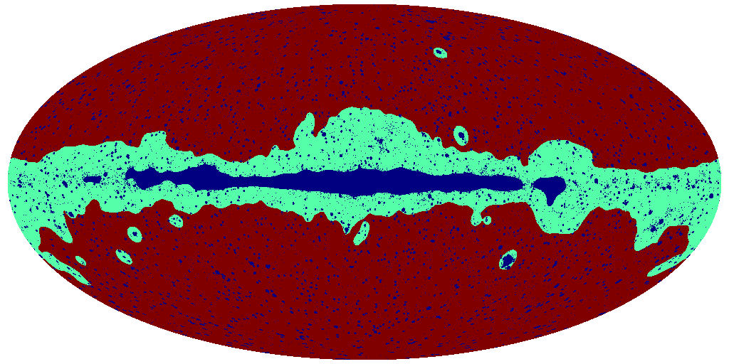
We compute localized statistics in both space and frequency: first the sphere is decomposed in three zones: a small zone where Galactic emission is so strong that no processing is attempted there, a second zone farther away from the Galactic center and finally a zone of weak Galactic emission which includes both ecliptic poles. The corresponding masks are shown on fig 3. We also localize in Fourier space by defining $Q=120$ domains which correspond to $120$ bins of angular frequency. The width $\delta_{\ell}$ of these spectral bins increases with the angular frequency $\ell$, as follows: $\delta_{\ell}=2$ for $0\leq\ell\leq 29$, $\delta_{\ell}=5$ for $30\leq\ell\leq 149$, $\delta_{\ell}=10$ for $150\leq\ell\leq 419$, $\delta_{\ell}=20$ for $420\leq\ell\leq 1199$, $\delta_{\ell}=50$ for $1200\leq\ell\leq 2000$.

For each of the two spatial domains, we build spectral statistics as follows: the zone of interest is isolated by using (an apodized version of) the masks shown on fig 3; the spherical harmonic coefficients for each of the 9 frequency channels are computed and collected in a $9\times 1$ vector $X_{lm}$ for each value of the pair $(\ell,m)$ up to $\ell_{\mathrm{max}}=2000$; spectral matrices are then computed for each $\ell\leq 2000$ as $\widehat{\mathbf{R}}_{\ell}=\frac{1}{2\ell+1}\sum_{m}X_{\ell m}X_{\ell m}^{\dagger}$. At this stage, since symmetric beams are assumed, their effect can be corrected as $\widehat{\mathbf{R}}_{\ell}\leftarrow W_{\ell}\widehat{\mathbf{R}}_{\ell}W_{\ell}$ where $W_{\ell}$ is a diagonal matrix. We also correct for incomplete sky coverage by dividing each $\mathbf{R}_{\ell}$ by a factor $f_{\mathrm{sky}}$ which is the fraction of the sky left after masking. Finally, the spectral matrices are binned into $\widehat{\mathbf{R}}_{q}=\frac{\sum_{\ell}h_{q}(\ell)(2\ell+1)\widehat{\mathbf{R}}_{\ell}}{\sum_{\ell}h_{q}(\ell)(2\ell+1)}$ where $h_{q}(\ell)$ is the top hat function for the $q$th bin. These matrices collect an effective number $p_{q}$ of Fourier modes given by $p_{q}=f_{\mathrm{sky}}\sum_{\ell}h_{q}(\ell)(2\ell+1)$.

5.3 Component analysis

We now fit a parametric model to the localized covariance matrices built at previous section. We fit independently the two zones of interest and then stitch the resulting maps together. In this illustrative example, we fit a model made of $C=4$ components

$$\mathbf{R}_{q}=\mathbf{R}_{q}^{\text{cmb}}+\mathbf{R}_{q}^{\text{sz}}+\mathbf{R}_{q}^{\text{gal}}+\mathbf{R}_{q}^{\text{noise}}\qquad 1\leq q\leq 120$$

with the following parametrization/constraints:

• The CMB component has a known emission law $\mathbf{a}_{\text{cmb}}$ but unknown angular spectrum $c(q)$ so $\mathbf{R}_{q}^{\text{cmb}}=\mathbf{a}_{\text{cmb}}\mathbf{a}_{\text{cmb}}^{\dagger}c_{\text{cmb}}(q)$ and $\theta^{\text{cmb}}=\bigl{\{}c_{\text{cmb}}(q)\bigl{\}}$.

• The SZ component, as the CMB, is fully coherent and has a known emission law. Hence, we take $\mathbf{R}_{q}^{\text{sz}}=\mathbf{a}_{\text{sz}}\mathbf{a}_{\text{sz}}^{\dagger}c_{\text{sz}}(q)$ and $\theta^{\text{sz}}=\bigl{\{}c_{\text{sz}}(q)\bigl{\}}$.

• We try to capture all Galactic emission (which is far from being coherent) together with emission from other galaxies – the ‘point source’ component, in a 4-dimensional component without other constraints, that is, we set up the ‘Galactic’ component model as $\mathbf{R}_{q}^{\text{gal}}=\mathbf{A}_{\text{gal}}\mathbf{P}_{q}\mathbf{A}_{\text{gal}}^{\dagger}$ with $\mathbf{A}_{\text{gal}}$ an unconstrained $9\times 4$ matrix and $\mathbf{P}_{q}$ a $4\times 4$ an unconstrained positive matrix so $\theta^{\text{gal}}=\bigl{\{}\mathbf{A}_{\text{gal}},\mathbf{P}_{q}\bigl{\}}$.

• For the noise contribution, we rely almost entirely on the instrument characterization: only $m$ global parameters are adjustable as described in the third example of component in section 3.2, that is we set up: $\mathbf{R}_{q}^{\text{noise}}=\mathrm{diag}(\alpha_{1}n_{1q}^{2},...,\alpha_{m}n_{mq}^{2})$ where $n_{iq}$ is known so $\theta^{\text{noise}}=\{\alpha_{i}\}$. The fixed spectra $n_{iq}$ are computed from the hit-counts maps and other figures given above.

Hence the global parameter vector is $\theta=[c_{\text{cmb}}(q),c_{\text{sz}}(q),\mathbf{A}_{\text{gal}},\mathbf{P}_{q},\alpha_{i}]$.

Note that the angular power spectrum of the cmb is obtained as a by-product of the global fitting procedure.

5.4 Some results

We show and comment some results from our best-fit model.

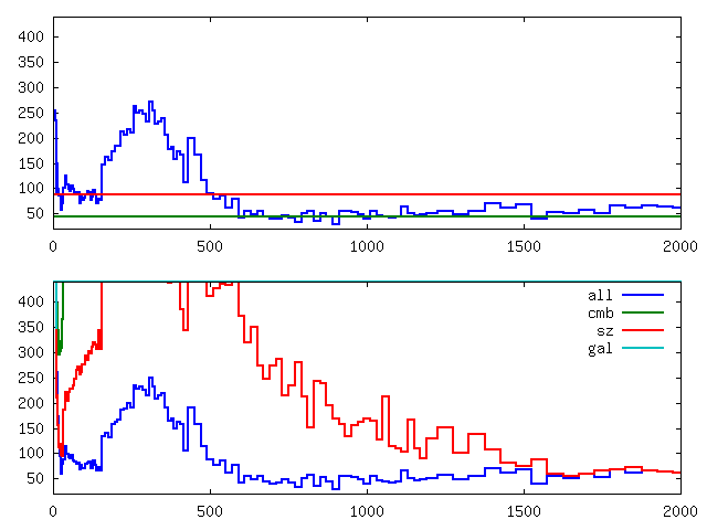
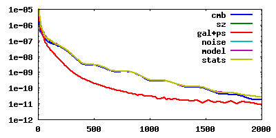
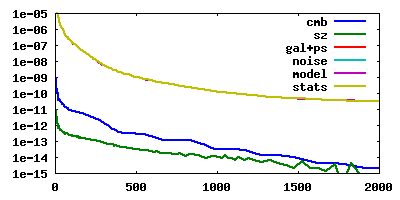
Goodness of fit. The top panel of figure 4 displays the values of $w_{q}K(\widehat{\mathbf{R}}_{q},\mathbf{R}_{q}(\hat{\theta}))$ versus the spectral domain index $q$ (actually: versus the average angular frequency $\ell$ for this domain). The overall mismatch measure $\phi(\theta)$ is just the sum of these quantities over all domains: see eq. (9). It is possible to predict the average mismatch value (in the asymptotic regime of many Fourier modes per domain) when the model holds. This provides at least a reference value in terms of goodness of fit. This value (and twice this value) are displayed as a horizontal line on fig. 4. The fit appears good for $\ell\geq 500$ but not so good for $200\leq\ell\leq 500$. This reflects the difficulty of modelling the complex galactic structure (since this component is important at this range scale) and also possibly the fact that the assumptions required for predicting the average mismatch are not met in this domain. The bottom panel of the figure shows how the mismatch increases when the contribution of any one of the components (except noise) is removed from the model. In this case, the mismatch explodes, showing that all fitted components are significant here.

Figure 4: Top: Spectral mismatch versus angular frequency for the best-fit model. Bottom: mismatch when any one of the components (but noise) is removed. See text for more details.

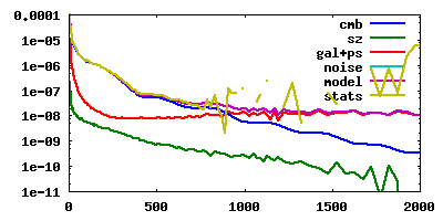
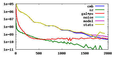
Power decomposition at sensor level. The decomposition (7) allows to find the contribution of each component on each detector by domain, i.e. as a function of angular frequency in the present case. Figure 5 displays for all detectors ($j=1,\ldots 9$) the values of $[\mathbf{R}_{q}^{c}(\hat{\theta})]_{jj}$ versus the center frequency of the $q$th spectral domain. In other words it shows estimated band-averaged angular spectra for all fitted components. It also shows the sum of these contributions over all components as well as the values of $[\widehat{\mathbf{R}}_{q}]_{jj}$. Actually the plot of the former quantity is almost entierly masked by the plot of the latter, evidencing a near perfect fit of the global angular spectrum.

Figure 5: Angular spectra on channels at 30, 70, 217, 857 GHz estimated with our best in the polar zone (mKRJ²). The line labelled stats shows the values of $[\widehat{\mathbf{R}}_{q}]_{jj}$; the line labelled model the values of $[\mathbf{R}_{q}(\hat{\theta})]_{jj}$; the latter is hidden by the former almost everywhere.

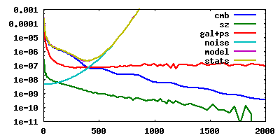
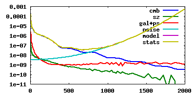
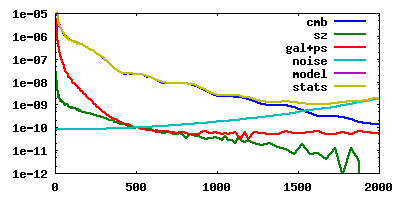
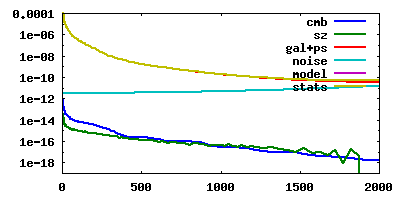
Figure 6 shows the cross-spectra between channels, that is the values of $[\mathbf{R}_{q}^{c}(\hat{\theta})]_{ij}$ for $4$ selected pairs of channels.

Figure 6: Cross-spectra for the channel pairs 30-70 GHz, 70-143 GHz, 143-353 GHz and 353-857 GHz and our fit with cmb+sz+(Galaxy+PS)+noise in polar zone (mKRJ²). Same conventions as in figure 5.

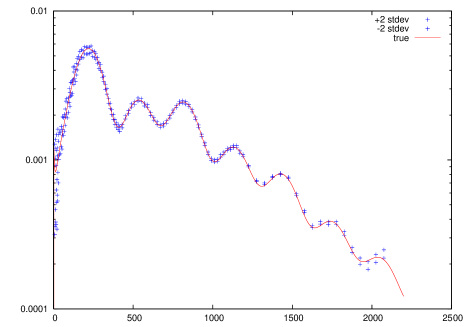
CMB angular spectra. Left panel of figure 7 shows the estimated angular spectrum $\hat{c}_{\ell}^{\mathrm{cmb}}$ with error bars computed from the Fisher information matrix. The angular spectrum of the CMB process is known in this simulated data set and displayed as a solid line. An excellent recovery is observed up to angular frequency $\ell=2000$, together with plausible error bars.

CMB map. The CMB map recovered through the localized Wiener filter (8) is shown in Figure 8. It has no visible contamination but reconstruction is not over the whole sky: the small Galactic region (shown on fig. 3) is not reconstructed because the Galactic emission is so strong that avoiding any contamination is very difficult. The bottom map of fig. 8 is the residual i.e. the error between true and reconstructed CMB maps. Some Galactic residuals are now visible indicating that the localization strategy should be improved (the Galactic emission is known to vary a lot across the sky, and especially near the Galactic plane).

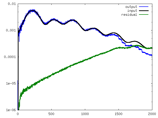
The angular spectrum of the residual map (CMB error map) is shown on the right panel of fig. 7. The linear (on this log scale) trend indicates that the error is noise-dominated (as also seen from the residual map).

Figure 7: Left: Estimated angular spectrum of the CMB (in polar zone) in mKCMB² with $\pm 2\sigma$ error bars given by the Fisher information matrix. We (conventionally) plot $\ell(\ell+1)c_{\ell}/2\pi$ rather than the plain angular spectrum $c_{\ell}$. Right: Angular spectrum of the reconstructed CMB and of the residual in mKCMB². The red and the black curves are the same reference input CMB spectrum which has been used to generate the CMB component.

Figure 8: Top: input CMB map; middle: estimated map outside of a small Galactic mask (color scale: $\pm 0.5$ mK CMB). Bottom: difference map (color scale: $\pm 0.05$ mK CMB).

Galactic and point source emission reconstruction. The most complex component is due to the radiation from the interstellar medium in our Galaxy (Galactic emission) as well as other galaxies (which contribute most of the emission of extragalactic ‘point sources’). The present work focuses on CMB reconstruction, and no attempt has been made to separate the Galactic emissions on the basis of the astrophysical radiation emission process (synchrotron emission, ‘free-free’ emission, or grey body emission from dust particles), nor on the basis of their origin (within our own Galaxy, or in other galaxies). For this reason, the sum of these emissions outside our Galactic + point source mask has been tentatively represented by a 4-dimensional ‘catch all’ model as explained above. The result of the separation for this component is shown in fig. 9. In spite of small discrepancies in the reconstruction on large angular scales, the result is quite satisfactory. Angular power spectra for this model, displayed in fig. 5 clearly correspond to the sum of the steep Galactic power spectrum, and a flat plateau at large angular frequency $\ell$, due to the contribution of emissions from the large number of extragalactic sources not masked by our point source mask.

Figure 9: The Galactic component seen by the 30, 70, 217 and 857 GHz channels. Left column: dust + free-free + synchrotron from the input maps in MJ/sr. Scale between 0 and 0.01 for the 30 and 70 GHz channels, between 0 and 0.1 for the 217 GHz channel and between 0 and 7 for the 857 GHz channel; center column: the 4-dimensional component found by SMICA with the same scale range; right column: the difference, rescaled by a factor of 10 to emphasize the errors.

6 Conclusion

The component separation technique discussed in this paper offers great modeling flexibility from the realization that separation can start with covariance matrix separation —i.e. the identification of individual component terms in the domain-wise decomposition (7)— followed by data separation according to (5). Too much flexibility may also introduce difficulties, though. Indeed, whether or not minimizing the covariance matching criterion $\phi(\theta)$ leads to uniquely identified components depends on the particular choice of component models. In our approach, however, the amount of constraints imposed on any component is fully tunable. By using more or less constrained components, the method ranges from totally blind to semi-blind, to non-blind.

Some other good points are the following. Speed: the method is potentially fast because large data sets are compressed into a much smaller set of covariance matrices. Accuracy: the method is potentially accurate because it can model complex components and then recover separated data via local Wiener filters which are naturally adapted to the local SNR conditions. Noise: the method can take noise into account without increased complexity since noise is not processed differently from any other component. Prior: the implementation also allows for easy inclusion of prior information about a component $c$ if it can be cast in the form of a prior probability distribution $p_{c}(\theta^{c})$ in which case one only need to subtracting $\log p_{c}(\theta^{c})$ from $\phi(\theta)$ and the related changes can be delegated to the component code. Varying resolution: in our application, and possibly others, the input channels are acquired by sensors with channel-dependent resolution. Accurate component separation requires to take this effect into account. This can be achieved with relative simplicity if the data coefficients entering in $\widehat{\mathbf{R}}_{q}$ are Fourier (or spherical harmonic) coefficients. Built-in goodness of fit via the mismatch measure (9).

This paper combines several ideas already known in the ICA literature: lumping together correlated components into a single multidimensional component is in [5]; minimization of a covariance-matching contrast $\phi(\theta)$ derived from the log-likelihood of a simple Gaussian model is found for instance in [17]; the extension to noisy models is already explained in [8]. The current paper goes one step further by showing how arbitrarily structured components can be separated and how the related complexity can be managed at the software level by a library of components.

About Gaussianity. The specific choice of the matching criterion (9) stems from a Gaussian model for the signal coefficients and the linear Wiener filter (5) is optimal only for Gaussian signals. Hence, there is no doubt that an improved statistical efficiency could be gained by resorting to non Gaussian models and to non-linear filtering for strongly non Gaussian data. However, this is more easily said than done, non Gaussian modeling/processing being often more difficult and costly to implement. By sticking to simple Gaussian assumptions, we can afford to model a non trivial correlation structure (through domains and through sensors) so it is not clear yet what the good trade-off is. It may depend very much on the scientific objectives (recovery of CMB versus recovery of other components, ability to predict estimation errors, …) and technical constraints (e.g. fast codes are important for assessment via Monte-Carlo runs). Intensive work is in progress within the Planck collaboration to assess the performance of various approaches for CMB analysis.

References

- [1] The Planck mission of ESA.
- [2] C. L. Bennett, R. S. Hill, G. Hinshaw, M. R. Nolta, N. Odegard, L. Page, D. N. Spergel, J. L. Weiland, E. L. Wright, M. Halpern, N. Jarosik, A. Kogut, M. Limon, S. S. Meyer, G. S. Tucker, and E. Wollack. First-Year Wilkinson Microwave Anisotropy Probe (WMAP) Observations: Foreground Emission. apjs, 148:97–117, September 2003.
- [3] A. Bonaldi, L. Bedini, E. Salerno, C. Baccigalupi, and G. de Zotti. Estimating the spectral indices of correlated astrophysical foregrounds by a second-order statistical approach. mnras, 373:271–279, November 2006.
- [4] F. R. Bouchet and R. Gispert. Foregrounds and CMB experiments I. Semi-analytical estimates of contamination. New Astronomy, 4:443–479, September 1999.
- [5] Jean-François Cardoso. Multidimensional independent component analysis. In Proc. ICASSP ’98. Seattle, pages 1941–1944, 1998.
- [6] J. Delabrouille, J.-F. Cardoso, and G. Patanchon. Multidetector multicomponent spectral matching and applications for cosmic microwave background data analysis. mnras, 346:1089–1102, December 2003.
- [7] Jacques Delabrouille and Jean-François Cardoso. Data Analysis in Cosmology, chapter Diffuse source separation in CMB observations. Lecture Notes in Physics. Springer, 2007. Editors: Vicent J. Martinez, Enn Saar, Enrique Martinez-Gonzalez, Maria Jesus Pons-Borderia.
- [8] Jacques Delabrouille, Jean-François Cardoso, and Guillaume Patanchon. Multi–detector multi–component spectral matching and applications for CMB data analysis. Monthly Notices of the Royal Astronomical Society, 346(4):1089–1102, December 2003. also available as http://arXiv.org/abs/astro-ph/0211504.
- [9] H. K. Eriksen, C. Dickinson, C. R. Lawrence, C. Baccigalupi, A. J. Banday, K. M. Górski, F. K. Hansen, E. Pierpaoli, and M. D. Seiffert. Bayesian foreground analysis with CMB data. New Astronomy Review, 50:861–867, December 2006.
- [10] K. M. Gorski et al. Healpix – a framework for high resolution discretization, and fast analysis of data distributed on the sphere. Astrophys. J., 622:759–771, 2005.
- [11] F. K. Hansen, A. J. Banday, H. K. Eriksen, K. M. Górski, and P. B. Lilje. Foreground Subtraction of Cosmic Microwave Background Maps Using WI-FIT (Wavelet-Based High-Resolution Fitting of Internal Templates). apj, 648:784–796, September 2006.
- [12] M. P. Hobson, A. W. Jones, A. N. Lasenby, and F. R. Bouchet. Foreground separation methods for satellite observations of the cosmic microwave background. mnras, 300:1–29, October 1998.
- [13] D. Maino, A. Farusi, C. Baccigalupi, F. Perrotta, A. J. Banday, L. Bedini, C. Burigana, G. De Zotti, K. M. Górski, and E. Salerno. All-sky astrophysical component separation with Fast Independent Component Analysis (FASTICA). mnras, 334:53–68, July 2002.
- [14] E. Martínez-González, J. M. Diego, P. Vielva, and J. Silk. Cosmic microwave background power spectrum estimation and map reconstruction with the expectation-maximization algorithm. mnras, 345:1101–1109, November 2003.
- [15] Lucas Parra and Clay Spence. Convolutive blind source separation of non-stationary sources. IEEE Trans. on Speech and Audio Processing, pages 320–327, may 2000.
- [16] Dinh-Tuan Pham and Jean-François Cardoso. Blind separation of instantaneous mixtures of non stationary sources. IEEE Trans. on Sig. Proc., 49(9):1837–1848, September 2001.
- [17] D.T. Pham. Blind separation of instantaneous mixture of sources via the Gaussian mutual information criterion. Signal Processing, (4):855–870, 2001.
- [18] H. Snoussi, G. Patanchon, J. F. Macías-Pérez, A. Mohammad-Djafari, and J. Delabrouille. Bayesian blind component separation for cosmic microwave background observations. In R. L. Fry, editor, Bayesian Inference and Maximum Entropy Methods in Science and Engineering, volume 617 of American Institute of Physics Conference Series, pages 125–140, May 2002.
- [19] V. Stolyarov, M. P. Hobson, M. A. J. Ashdown, and A. N. Lasenby. All-sky component separation for the Planck mission. mnras, 336:97–111, October 2002.
- [20] M. Tegmark and G. Efstathiou. A method for subtracting foregrounds from multifrequency CMB sky maps. mnras, 281:1297–1314, August 1996.
- [21] M. Tegmark, D. J. Eisenstein, W. Hu, and A. de Oliveira-Costa. Foregrounds and Forecasts for the Cosmic Microwave Background. apj, 530:133–165, February 2000.