Dynamical Aspects of 2D Quantum Percolation

Abstract

The existence of a quantum percolation threshold $p_{q}<1$ in the 2D quantum site-percolation problem has been a controversial issue for a long time. By means of a highly efficient Chebyshev expansion technique we investigate numerically the time evolution of particle states on finite disordered square lattices with system sizes not reachable up to now. After a careful finite-size scaling, our results for the particle’s recurrence probability and the distribution function of the local particle density give evidence that indeed extended states exist in the 2D percolation model for $p<1$.

I Introduction

For classical percolation above a critical concentration of accessible sites, the so-called percolation threshold $p_{c}$, a spanning cluster exists, allowing for transport. In the quantum case, however, the existence of the spanning cluster does not guarantee an extended wave function. As for the Anderson Anderson (1958) and binary alloy Alvermann and Fehske (2005) disorder models scattering and interference effects at the irregular boundaries of the cluster may lead to localization of the quantum particle, i.e. absence of diffusion. Increasing the concentration of accessible sites $p$ above $p_{c}$, the first occurrence of extended states defines a quantum percolation threshold, $p_{q}$. For the Anderson model, below a critical disorder strength, a single mobility edge separates bands of localized and extended states. By contrast, for the binary alloy and three-dimensional (3D) percolation model a sequence of “mobility edges” exists Schubert et al. (2005a). It is clear that $p_{c}\leq p_{q}\leq 1$ and the fundamental question is, of course, whether $p_{q}$ equals one of these boundaries.

For the 3D case, results in the literature Koslowski and von Niessen (1990); Soukoulis et al. (1992); Schubert et al. (2005a) agree on $p_{c}^{3D}<p_{q}^{3D}<1$, with estimates for $p_{q}^{3D}$ ranging from $0.4$ to $0.5$ for site percolation on a simple cubic lattice. In 2D, the situation is less clear. Here the physical community is evenly divided: one group Soukoulis and Grest (1991); Mookerjee et al. (1995); Bunde et al. (1998); Hałdas et al. (2002) favors $p_{q}^{2D}=1$ while another group Odagaki and Chang (1984); Srivastava and Chaturvedi (1984); Letz and Ziegler (1999); Daboul et al. (2000); Eilmes et al. (2001); Nazareno et al. (2002); Islam and Nakanishi (2007) claims that $p_{q}^{2D}<1$. The most striking argument against $p_{q}^{2D}<1$ comes from one-parameter scaling theory Abrahams et al. (1979), according to which arbitrary small disorder always leads to localization in 2D. Nevertheless, there are hints for $p_{q}^{2D}<1$. In this regard band center states seem to be of particular importance Inui et al. (1994); Eilmes et al. (1998). Whether $E=0$ states on a 2D bipartite depleted square lattice are a possible “let out clause” Gade and Wegner (1991); Gade (1993) for the one-parameter scaling theory result is an open question.

Renewed interest in 2D quantum percolation came up in connection with the unusual transport properties of novel materials. For example, the metal-insulator transition in perovskite manganite films and the related colossal magnetoresistance effect seems to be inherently percolative Zhang et al. (2002); Becker et al. (2002). Quantum percolation might be of importance for the experimentally observed metallic behavior of dilute weakly disordered Si-MOSFETs Abrahams et al. (2001). Moreover, quite recently, a quantum percolation scenario has been proposed for minimal conductivity in undoped graphene Cheianov et al. (2007). All this gives additional motivation for the rather fundamental study of 2D quantum percolation presented in this work.

II Model and methods

We start from a tight-binding Hamiltonian of non-interacting spinless fermions in Wannier representation

$${H}=\sum_{i=1}^{N}\epsilon_{i}{d}_{i}^{{\dagger}}{d}_{i}-t\sum_{\langle ij\rangle}({d}_{i}^{{\dagger}}{d}_{j}+\text{H.c.})\,,$$ (1)

with uniform hopping $t$ between nearest neighbors $\langle ij\rangle$ on a finite square lattice with $N=L^{2}$ sites and periodic boundary conditions. The on-site energies $\epsilon_{i}$ are subject to the bimodal distribution

$$p[\epsilon_{i}]=p\,\delta(\epsilon_{i}-\epsilon_{A})+(1-p)\,\delta(\epsilon_{i}-\epsilon_{B})\,.$$ (2)

The quantum site-percolation Hamiltonian then is obtained in the limit $|\epsilon_{B}-\epsilon_{A}|\to\infty$. Without loss of generality we choose $\epsilon_{A}=0$. In this situation the fermions move on a random assembly of $A$-lattice points. Depending on $p$, the largest cluster of $\bar{N}$ connected $A$-sites may span the entire lattice. Note that the dynamics of our finite system is governed by two different time scales. The time scale of a hopping process is given by the inverse of the hopping matrix element, $\tau_{0}=1/t$. To account for the system size, we define a characteristic time $\bar{T}_{0}=\bar{N}\tau_{0}$, which, in principle, is necessary to visit each site of the spanning cluster once.

In order to address the problem of localization in quantum percolation, we determine, for $p>p_{c}=0.593$, the recurrence probability of a particle to a given site, $P_{R}(\tau)$, which for $\tau\to\infty$ may serve as a criterion for Anderson localization Kabanov and Mashtakov (1993); Janssen (1998). While for extended states on the spanning cluster $P_{R}(\tau\to\infty)=1/\bar{N}$ scales to zero in the thermodynamic limit, for localized states $P_{R}(\tau)$ remains finite as $\bar{N}\to\infty$.

Conceptionally, in a first step, we track the time evolution of an initially localized state (which, of course, in general is not an eigenstate) by calculating the modulus square of the wave function at the particle’s starting position as a function of time $\tau$. To this end we expand the time evolution operator $U(\tau)={\mathrm{e}}^{-{\mathrm{i}}H\tau}$ in Chebyshev polynomials Tal-Ezer and Kosloff (1984); Chen and Guo (1999); Weiße and Fehske (2008), where the Hamiltonian has to be rescaled to the definition interval of the Chebyshev polynomials $T_{k}$, $[-1,1]$. With $H=a\tilde{H}+b$ we obtain

$$U(\tau)={\mathrm{e}}^{-{\mathrm{i}}b\tau}\left[c_{0}(a\tau)+2\sum\limits_{k=1}^{M}c_{k}(a\tau)T_{k}(\tilde{H})\right]\;.$$ (3)

The expansion coefficients $c_{k}$ are given by

$$c_{k}(a\tau)=\int\limits_{-1}^{1}\dfrac{T_{k}(x)e^{-{\mathrm{i}}a\tau x}}{\pi\sqrt{1-x^{2}}}{\mathrm{d}}x=(-{\mathrm{i}})^{k}J_{k}(a\tau)\;,$$ (4)

where $J_{k}$ denotes the Bessel function of the first kind. To calculate the evolution of a state $|\psi(\tau)\rangle$ from one time grid point to the next, $|\psi(\tau+\Delta\tau)\rangle=U(\Delta\tau)|\psi(\tau)\rangle$, we have to accumulate the $c_{k}$-weighted contributions of the different orders $|v_{k}\rangle=T_{k}(\tilde{H})|\psi(\tau)\rangle$. As the coefficients $c_{k}(a\Delta\tau)$ depend on the time step but not on time explicitly, we need to calculate them only once. The contributions $|v_{k}\rangle$ can then be calculated iteratively using the recurrence relation of the Chebyshev polynomials

$$|v_{k+1}\rangle=2\tilde{H}|v_{k}\rangle-|v_{k-1}\rangle\;,$$ (5)

where $|v_{1}\rangle=\tilde{H}|v_{0}\rangle$ and $|v_{0}\rangle=|\psi(\tau)\rangle$. Due to the fast asymptotic decay of the Bessel functions

$$J_{k}(a\tau)\sim\frac{1}{\sqrt{2\pi k}}\left(\frac{{\mathrm{e}}a\tau}{2k}\right)^{k}\quad\text{for}\quad k\to\infty\;,$$ (6)

the coefficients $c_{k}$ vanish rapidly above a certain expansion order. As a result from the infinite series only a finite number of $M$ terms needs to be taken into account. Clearly $M$ depends on the time step used. Truncating the series for large $a\tau>10^{3}$ at $M\sim 1.5a\tau$, the $|c_{k}|<10^{-16}$ for all discarded terms. For even larger values of $a\tau$, the necessary value of $M/(a\tau)$ is even reduced and approaches $M\sim a\tau$ for $\tau\to\infty$. Thus, as compared to the standard Crank-Nicolson algorithm, the Chebyshev expansion permits the use of a considerably larger time step to achieve the same accuracy, i.e. allows for a very efficient calculation of the time evolution of a given state.

In a second step, we employ the so-called local distribution approach Alvermann and Fehske (2006, 2008). In the theoretical investigation of disordered systems it turns out that the distribution of random quantities is central. While all characteristics of a certain material are determined by the distribution $p[\epsilon_{i}]$, each actual sample constitutes only one particular realization $\{\epsilon_{i}\}$. At each randomly chosen site $i$ of such a particular sample, we observe different local environments. That is disorder breaks translational invariance and we have to focus on site-dependent quantities like the local density of states (LDOS) Schubert et al. (2005b) at site $i$

$$\rho_{i}(E)=\sum\limits_{m=1}^{\bar{N}}|\langle i|m\rangle|^{2}\,\delta(E-E_{m})\;.$$ (7)

Given an energy $E$, the LDOS can be efficiently calculated by means of the kernel polynomial method Weiße et al. (2006). Considering the LDOS, a well established criterion for localization is the following. Probing different sites in the sample and recording the values of $\rho_{i}$ gives the probability distribution $f[\rho_{i}]$. To alleviate the problem of statistical noise one usually considers instead of $f[\rho_{i}]$ the distribution function

$$F[\rho_{i}]=\int_{0}^{\rho_{i}}f[\rho_{i}^{\prime}]\,{\mathrm{d}}\rho_{i}^{\prime}\;.$$ (8)

In the thermodynamic limit both $f[\rho_{i}]$ and $F[\rho_{i}]$ are independent of the actual realization $\{\epsilon_{i}\}$ (i.e. self-averaging), but solely depend on $p[\epsilon_{i}]$. Therefore $F[\rho_{i}]$ characterizes $H(p[\epsilon_{i}])$, not only $H(\{\epsilon_{i}\})$. That means, at the level of distributions, we have restored translational invariance. For an extended state the amplitude of the wave function is more or less uniform and $f[\rho_{i}]$ is sharply peaked and symmetric around its mean value $\langle\rho_{i}\rangle$. For localized states $\rho_{i}$ strongly fluctuates throughout the lattice, giving rise to a very asymmetric $f[\rho_{i}]$ with a long tail and $\langle\rho_{i}\rangle\to 0$. Consequently the distribution function $F[\rho_{i}]$ steeply rises for extended states whereas for localized states the increase extends over several orders of magnitude. These arguments also hold for the (time-dependent) particle density at site $i$

$$n_{i}(\tau)=\Big{|}\sum\limits_{m=1}^{\bar{N}}{\mathrm{e}}^{-{\mathrm{i}}E_{m}t}\langle m|\psi(0)\rangle\langle i|m\rangle\Big{|}^{2}\;,$$ (9)

if we take additional care of some aspects. Evolving an arbitrary initial state $|\psi(0)\rangle$ in time, we only have access to $n_{i}(\tau)$, containing contributions of the whole spectrum. Calculating the time evolution of an initial state we have access to $n_{i}$ on the whole cluster, which gives a much better statistics. On the other hand, the chosen initial conditions introduce an additional dependency. Especially for localized states the local environment of the starting position will influence $F[n_{i}]$. So for $n_{i}$, in addition to taking the thermodynamic limit, we have to examine different initial conditions. While the LDOS approach allows for an energy resolved examination of the localization problem, $n_{i}$ gives no information about $p_{q}(E)$ because it contains contributions from all $E$. But, starting from $p_{c}$ and increasing $p$, we detect at a certain $p=p_{q}$ the first occurrence of extended states somewhere in the spectrum.

III Results

Figure 1: (Color online) Time evolution of the normalized local particle density $\bar{N}n_{i}(\tau)$ for an initially localized state on the spanning cluster of a $N=512^{2}$ square lattice for $p=0.65$ (left) and $p=0.90$ (right). Due to normalization, for an extended state evenly spread over all sites of the spanning cluster this quantity is equal to unity.

Figure 2: (Color online) Time evolution of the distribution function of the local particle density, $F[\bar{N}n_{i}(\tau)]$. The curves correspond to the data in Fig. 1, supplemented by the distribution functions at $\tau=0$ (dot-double-dashed curve).

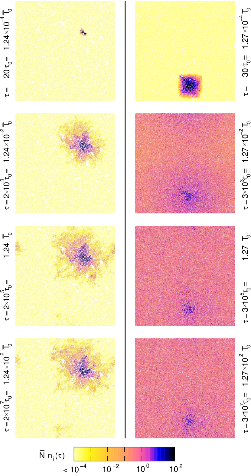
Let us now discuss the outcome of our numerical investigations. Figure 1 compares the time evolution of an initially localized state on the spanning cluster for low (left panels) and high (right panels) concentration of $A$ sites, for which qualitatively different behaviors emerge. For small $p=0.65>p_{c}$, the initial state spreads within a short time over a finite region of the spanning cluster. But also for very long times, $\tau>100\bar{T}_{0}$, this extension does not change significantly anymore. For larger $p$, the spreading is even faster. In contrast to the previous case, for $p=0.90$ the state is not confined to some finite region, but $n_{i}$ is transfered to the whole cluster. Since the initial state is a superposition of eigenstates from the whole spectrum, it also contains contributions from localized states, for instance near the band edges. Those are reflected in the darker spots in the vicinity of the initial position, which persist there, even for very long times. This signature of localized states we already know from the case of small $p$. The essential new feature is that for large $p$ some eigenstates exist, which are not localized, i.e. spread over the whole cluster.

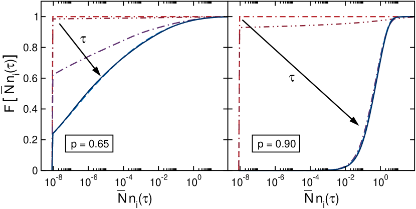
To go beyond this simple visualization and account for a quantitative description, in Fig. 2 we show the corresponding local particle density distribution functions $F[n_{i}]$. The different behavior of localized and extended states becomes obvious as the time increases. Since these results were obtained for a particular sample and a certain starting position it is necessary to ask how strong these findings depend on the initial conditions, and if they are representative for the underlying $p[\epsilon_{i}]$.

To answer this question we examine systematically the influence of the initial conditions on the behavior of the state. In this respect the geometry and energy of the initial state, the starting position on the cluster as well as the particular cluster realization $\{\epsilon_{i}\}$ should be of importance. A fingerprint in which all these aspects come into play is the LDOS of the initial state.

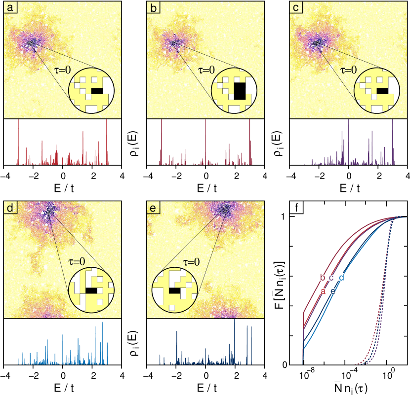
In Fig. 3 we examine the influence of these issues one by one. Fixing a particular cluster realization and starting position of the wave function, we may construct several initial states with the same total energy. This can be done by choosing a different number of sites which initially have non-vanishing amplitudes. For a state with finite amplitude only on two neighboring sites, $a$ and $\sqrt{1-a^{2}}$, respectively, we get $E=2ta\sqrt{1-a^{2}}$ and we may continuously tune $E\in[-t,t]$ by choice of $a$ (cf. Fig. 3 a and c). These energies may also be constructed for more complicated initial states, as e.g. for the one shown in Fig. 3 b, with non-vanishing amplitudes on six adjacent sites. The more complicated these structures get and the more sites are involved, the larger energies of the initial state are possible, e.g. for the configuration of Fig. 3 b up to $(1+\sqrt{2})t$. As stressed above, these energies are not eigenenergies of $H$, i.e. the initial state is a superposition of eigenstates from the whole spectrum. A quantitative characterization of the amount of different contributions can be obtained by the LDOS of the initial state. Changing the starting position (Fig. 3 d) or the cluster realization (Fig. 3 e) has a similar effect. Essentially, we see the same behavior as for the changes in Figs. 3 a-c. Most notably, although the LDOS at $\tau=0$ and the evolution of the states differs in detail, on a coarse grained scale they behave similarly. This is also corroborated by the behavior of the distribution function $F[n_{i}(\tau)]$ for sufficient long times $\tau$. Despite minor differences between the five curves, they agree on showing the characteristics of a localized state (Fig. 3 f, solid lines). The more a state is localized, i.e. the lower $p$, the more the local structure of the spanning cluster influences its evolution and thus $F[n_{i}(\tau)]$. At large $p$, the dependency of an extended state on the above criteria is much weaker, as in this case the local environment of the starting position is less important (Fig. 3 f, dashed lines). Overall, the characteristics of the time evolution is mainly determined by the cluster structure, the initial state has only minor influence. This holds as the random nature of the cluster guarantees a similar structure above a certain scale. Finally one may ask if the chosen boundary conditions or the linear extension (odd/even) of the lattice influences the dynamics. The latter distinction has been shown to be important for a bond percolation model because of the bipartiteness of the underlying lattice Soukoulis et al. (1982). In our case, however, we did not see an influence on the results.

Figure 3: (Color online) Influence of the initial conditions on the evolution of the wave function on a $N=512^{2}$ system at $p=0.65$. The colormap is the same as the one in Fig.1. Panels a-d show the same cluster realization, with identical starting positions for a-c. All states have $E=0.5t$, except for the case shown in panel c, where $E=t$. The insets give a magnification of $n_{i}(0)$. The corresponding LDOS of the initial states are given below each panel. In panel f the solid lines show the distribution function $F[n_{i}(\tau)]$ for $\tau=15.4\bar{T}_{0}$. For comparison the dashed lines indicate $F[n_{i}(\tau)]$ for $p=0.90$ subject to the same differences in the initial conditions.

Figure 4: (Color online) $L_{2}$ norm of the difference between the distribution function $F[n_{i}(\tau)]$ at time $\tau$ and the quasi-stationary distribution $F[n_{i}(\tau^{*})]$ for different system sizes. The inset shows the dependency of this quantity on the time difference for the $N=4096^{2}$ system in the quasi-stationary regime. Note the different axis scales.

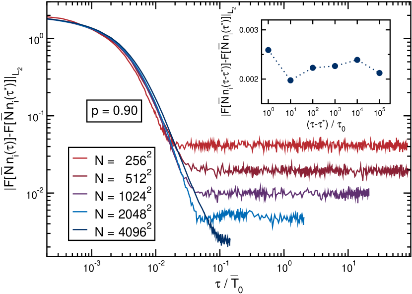
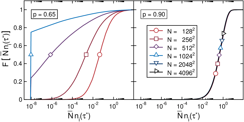
In view of a finite-size scaling of the numerical data we first have to ensure that the obtained distribution function has already become quasi-stationary. To check this, we calculate the $L_{2}$ norm of the difference between two distribution functions at different times. Due to fluctuations, we cannot expect this quantity to vanish completely even for large times. For $\tau\gtrsim\tau^{*}\approx 0.1\bar{T}_{0}$, however, we have reached the quasi-stationary regime for all considered system sizes (cf. Fig. 4). At this time, the wave function has reached its maximum extension and the further development is governed by amplitude fluctuations from site to site. In this regime, the difference between the distribution functions does not depend on time anymore (inset of Fig. 4), which is a clear indication of random fluctuations without additional drift motion. This allows for a determination of the quasi-stationary distribution function together with an error estimation and enables us to compare different system sizes. In view of computation time, the scaling $\tau^{*}\sim\bar{T}_{0}\sim\bar{N}$ together with the linear dependency on the dimension of the Hilbert space for the Chebyshev expansion leaves us with a scaling $\sim(pN)^{2}\sim p^{2}L^{4}$.

As soon as we have quasi-stationary distribution functions, their dependency on the system size may be exploited for a quantitative distinction between localized and extended states (Fig. 5). For the two different occupation probabilities, we observe completely different behavior: while for $p=0.65$ the distribution function shifts towards smaller values on increasing the system size, for $p=0.90$ it is not affected by the change of system size at all. The latter is clearly the behavior one would expect for an extended state.

Figure 5: (Color online) Finite-size scaling of $F[\bar{N}n_{i}(\tau^{*})]$ in the quasi-stationary regime.

IV Conclusion

To summarize, we applied a highly efficient Chebyshev expansion technique to calculate the dynamics of particle states for the 2D quantum site-percolation model. The local particle density contains contributions of eigenstates from the whole energy spectrum and is therefore an ideal tool to globally investigate the localization properties of the system. Examining the corresponding distribution function allows for a distinction between localized and extended states. Above a certain concentration of accessible sites the shape of the distribution function becomes independent of the system size. This gives evidence that there are (some) extended states in the spectrum. Having access to much larger systems than any others previously in the literature, we conclude from our data, supplemented by a careful finite-size scaling, that $p_{q}^{2D}<1$.

Acknowledgments

We thank J. Kantelhardt for helpful discussion. The numerical calculations have been performed on the HLRB at LRZ Munich and the TeraFlop compute cluster at the Institute of Physics, Greifswald University.

References

- Anderson (1958) P. W. Anderson, Phys. Rev. 109, 1492 (1958).
- Alvermann and Fehske (2005) A. Alvermann and H. Fehske, Eur. Phys. J. B 48, 295 (2005).
- Schubert et al. (2005a) G. Schubert, A. Weiße, and H. Fehske, Phys. Rev. B 71, 045126 (2005a).
- Koslowski and von Niessen (1990) T. Koslowski and W. von Niessen, Phys. Rev. B 42, 10342 (1990).
- Soukoulis et al. (1992) C. M. Soukoulis, Q. Li, and G. S. Grest, Phys. Rev. B 45, 7724 (1992).
- Soukoulis and Grest (1991) C. M. Soukoulis and G. S. Grest, Phys. Rev. B 44, 4685 (1991).
- Mookerjee et al. (1995) A. Mookerjee, I. Dasgupta, and T. Saha, Int. J. Mod. Phys. B 9, 2989 (1995).
- Bunde et al. (1998) A. Bunde, J. W. Kantelhardt, and L. Schweitzer, Ann. Phys. (Leipzig) 7, 372 (1998).
- Hałdas et al. (2002) G. Hałdas, A. Kolek, and A. W. Stadler, Phys. Status Solidi B 230, 249 (2002).
- Odagaki and Chang (1984) T. Odagaki and K. C. Chang, Phys. Rev. B 30, 1612 (1984).
- Srivastava and Chaturvedi (1984) V. Srivastava and M. Chaturvedi, Phys. Rev. B 30, 2238 (1984).
- Letz and Ziegler (1999) M. Letz and K. Ziegler, Philos. Mag. B 79, 491 (1999).
- Daboul et al. (2000) D. Daboul, I. Chang, and A. Aharony, Eur. Phys. J. B 16, 303 (2000).
- Eilmes et al. (2001) A. Eilmes, R. A. Römer, and M. Schreiber, Physica B 296, 46 (2001).
- Nazareno et al. (2002) H. N. Nazareno, P. E. de Brito, and E. S. Rodrigues, Phys. Rev. B 66, 012205 (2002).
- Islam and Nakanishi (2007) M. F. Islam and H. Nakanishi (2007), preprint, URL arXiv:0709.4085v1.
- Abrahams et al. (1979) E. Abrahams, P. W. Anderson, D. C. Licciardello, and T. V. Ramakrishnan, Phys. Rev. Lett. 42, 673 (1979).
- Inui et al. (1994) M. Inui, S. A. Trugman, and E. Abrahams, Phys. Rev. B 49, 3190 (1994).
- Eilmes et al. (1998) A. Eilmes, R. A. Römer, and M. Schreiber, Phys. Status Solidi B 205, 229 (1998).
- Gade and Wegner (1991) R. Gade and F. Wegner, Nucl. Phys. B 360, 213 (1991).
- Gade (1993) R. Gade, Nucl. Phys. B 398, 499 (1993).
- Zhang et al. (2002) L. Zhang, C. Israel, A. Biswas, R. L. Greene, and A. de Lozanne, Science 298, 805 (2002).
- Becker et al. (2002) T. Becker, C. Streng, Y. Luo, V. Moshnyaga, B. Damaschke, N. Shannon, and K. Samwer, Phys. Rev. Lett. 89, 237203 (2002).
- Abrahams et al. (2001) E. Abrahams, S. V. Kravchenko, and M. P. Sarachik, Rev. Mod. Phys. 73, 251 (2001).
- Cheianov et al. (2007) V. V. Cheianov, V. I. Fal’ko, B. L. Altshuler, and I. L. Aleiner (2007), URL arXiv:0706.2968v2.
- Kabanov and Mashtakov (1993) V. V. Kabanov and O. Y. Mashtakov, Phys. Rev. B 47, 6060 (1993).
- Janssen (1998) M. Janssen, Physics Reports 295, 1 (1998).
- Tal-Ezer and Kosloff (1984) H. Tal-Ezer and R. Kosloff, J. Chem. Phys. 81, 3967 (1984).
- Chen and Guo (1999) R. Chen and H. Guo, Comp. Phys. Comm. 119, 19 (1999).
- Weiße and Fehske (2008) A. Weiße and H. Fehske, Lecture Notes in Physics 739, 545 (2008).
- Alvermann and Fehske (2006) A. Alvermann and H. Fehske, J. Phys.: Conf. Ser. 35, 145 (2006).
- Alvermann and Fehske (2008) A. Alvermann and H. Fehske, Lecture Notes in Physics 739, 505 (2008).
- Schubert et al. (2005b) G. Schubert, A. Weiße, G. Wellein, and H. Fehske, in High Performance Computing in Science and Engineering, Garching 2004, edited by A. Bode and F. Durst (Springer-Verlag, Heidelberg, 2005b), pp. 237–250.
- Weiße et al. (2006) A. Weiße, G. Wellein, A. Alvermann, and H. Fehske, Rev. Mod. Phys. 78, 275 (2006).
- Soukoulis et al. (1982) C. M. Soukoulis, I. Webman, G. S. Grest, and E. N. Economou, Phys. Rev. B 26, 1838 (1982).