July 2008
Probing the Effective Number of Neutrino Species with Cosmic Microwave Background
Kazuhide Ichikawa1,2, Toyokazu Sekiguchi1, and Tomo Takahashi3
1
Institute for Cosmic Ray Research,
University of Tokyo, Kashiwa 277-8582, Japan
2
Department of Physics and Astronomy, University College London, Gower Street, London, WC1E 6BT, U.K.
3
Department of Physics, Saga University, Saga 840-8502, Japan
We discuss how much we can probe the effective number of neutrino species with cosmic microwave background alone. Using the data of WMAP, ACBAR, CBI and BOOMERANG experiments, we obtain a constraint on the effective number of neutrino species as at 95 % C.L. for a power-law CDM flat universe model. The limit is improved to be at 95 % C.L. if we assume that the baryon density, and the helium abundance are related by the big bang nucleosynthesis theory. We also provide a forecast for the PLANCK experiment using a Markov chain Monte Carlo approach. In addition to constraining , we investigate how the big bang nucleosynthesis relation affects the estimation for these parameters and other cosmological parameters.
1 Introduction
Cosmology is now becoming a precision science, and cosmological observations can give us a lot of information for our understanding of the universe. Moreover, the interplay between cosmology and particle physics in various contexts has also been discussed vigorously. One of such examples is the effective number of neutrino species . Although collider experiments such as LEP have measured the number of light active neutrino types to be [1], it is important to cross-check this value because cosmological measurements may lead to different value. This could be due to an extra radiation component which is predicted by some models of particle physics such as sterile neutrinos (see Ref. [2] and references therein), or due to incomplete thermalization of neutrinos in the low-scale reheating universe in which the reheating temperature can be as low as MeV and is predicted to be less than three [3, 4, 5, 6]. If such a non-standard ingredient exists, it can affect big bang nucleosynthesis (BBN), cosmic microwave background (CMB), large scale structure (LSS) and so on; thus precise cosmological observations can probe these scenarios through the effective number of neutrino species.
Constraints on have been investigated in the literature using the information of CMB and LSS, sometimes with priors on the Hubble constant, cosmic age and Helium abundance [7, 8, 9, 10, 11, 12, 13, 14, 15, 16, 17, 18, 19, 20, 21, 22, 23, 24, 25, 26, 27, 28, 29, 30]. Although CMB in general can constrain various quantities severely, since the effects of on CMB are degenerate with some cosmological parameters, the studies so far have combined CMB data with some other observations such as LSS to obtain a sensible constraint on . However, when one uses the data from LSS, constraints can become different depending on how one treats non-linear correction/bias on small scales for the matter power spectrum [23]. Furthermore, different LSS data seem to give different constraints on [16, 17, 20, 21, 23]. Regarding the prior on the Hubble constant , as is summarized in Ref. [20], it can yield some constraints on when combined with CMB data (without LSS data) [8, 9, 10, 12, 13], but they depend on the prior adopted. One may consider that we can use the usually assumed prior on the Hubble constant based on the result by Freedman et al. [31], but another group reported a somewhat lower value as [32]. If the lower value for is adopted as the prior, a resulting constraint on would be different. Having these considerations in mind, it is desirable to investigate a constraint on without these kind of uncertainties.
In this paper, we study a constraint on from CMB experiments alone. By making the analysis of CMB data alone, we can avoid such subtleties as the galaxy-bias/non-linear corrections and the value for the prior on the Hubble constant. However, as is mentioned above, the effects of are strongly degenerate in CMB with other cosmological parameters such as energy density of matter, the Hubble constant, and the scalar spectral index, and, in fact, we could not obtain a meaningful bound only with WMAP3 [20, 23]. Recent WMAP5 alone analysis gives a better constraint but it still cannot give an upper bound [28, 27]. As we will discuss later, the degeneracy is significant up to about the 2nd/3rd peak of the CMB power spectrum where the observation of WMAP has precisely measured. To break this degeneracy to some extent, it would be helpful to have the information at higher multipoles where signals unique to relativistic neutrinos are expected to appear [33]. Recently, the data from ACBAR which probes CMB at higher multipoles than those of WMAP has been updated [34]. By using this data in addition to other small scale observations such as BOOMERANG and CBI, we can obtain a relatively severe constraint on which is comparable to that have been obtained previously with LSS data.
The organization of this paper is as follows. In the next section, we start with the discussion how affects the CMB power spectrum, which helps to understand our results for the constraint on . In Section 3, we study the current constraint on using observations of CMB alone. We use the data from WMAP5, the recent ACBAR, BOOMERANG and CBI. Furthermore, we forecast the constraint from the future Planck experiment. In the final section, we summarize our results and discuss its implications for some models of particle physics/the early universe.
2 Effects of on CMB
The effective number of neutrino species represents the energy density stored in relativistic components as
| (1) |
where , and are energy densities of photons, three species of massless active neutrinos and some possible extra radiation components, respectively. In this paper, we assume that neutrinos are massless and have no chemical potential. For the case with the standard three neutrino flavors without an extra relativistic component, the effective number of neutrino is where some corrections from the incomplete decoupling due to a slight interaction of neutrinos with electrons/positrons and finite temperature QED effect to the electromagnetic plasma are taken into account [35]. Any deviation of from this value implies that there exists an extra relativistic component and/or some non-standard thermal history takes place such as the low reheating temperature scenario.
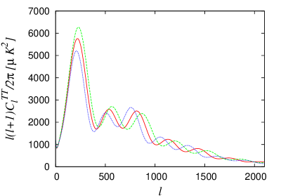
To illustrate the effects of on CMB, we plot CMB power spectra for several values of in Fig. 1. Other cosmological parameters are assumed as the mean values of WMAP5 alone analysis for a power-law flat CDM model. As seen from the figure, as we increase the value of , the height of the 1st peak is strongly enhanced and the positions of acoustic peaks are shifted to higher multipoles. Also, the amplitude on small scales (higher multipoles) is suppressed. Below, we discuss where these changes are coming from.
One of the main effects of comes from the change of the epoch of the radiation-matter equality. By increasing (decreasing) the value of , the radiation-matter equality occurs later (earlier). Thus the increase (decrease) of gives an almost the same effect of the decrease (increase) of energy density of matter. One of noticeable features is that the height of the first acoustic peak is enhanced by increasing the value of . This is due to the early integrated Sachs-Wolfe (ISW) effect in which fluctuations of the corresponding scale, having crossed the sound horizon in the radiation-dominated epoch are boosted by the decay of the gravitational potential. Thus a larger amount of relativistic species drives the first peak higher. Another effect is the shift of the position of acoustic peaks due to the change of the radiation-matter equality through the change of . The position of acoustic peaks is well captured by the so-called acoustic scale which is inversely proportional to the peak position and written as
| (2) |
where and are the comoving angular diameter distance to the last scattering surface and the sound horizon at the recombination epoch , respectively. Although almost remains the same for different values of , becomes smaller when is increased. Thus the positions of acoustic peaks are shifted to higher multipoles (smaller scales) by increasing the value of . Furthermore, since the position of the -th peak can be roughly written as , separations of the peaks become also greater for larger .
Another important effect is free-streaming of ultrarelativistic neutrinos [33]. The perturbation of ultrarelativistic neutrino propagates with the speed of light, which is faster than the sound speed of acoustic oscillations of photon-baryon fluid. The coupled photon-baryon component behaves to oscillate like a compressional fluid; on the other hand, ultrarelativistic neutrinos free-stream to erase their fluctuations. These two components are coupled via gravity; thus the fluctuations of photons can also be affected by the free-streaming of neutrinos, which results in the damping of the amplitude and the shift of the acoustic oscillations. The effects are significant on small scales where fluctuations of a given scale enter the horizon while the energy density of ultrarelativistic neutrinos takes a significant portion of that of the universe.
Although the effects of the standard cosmological parameters on the heights and positions of acoustic peaks are well known, here we discuss them in some phenomenological way including the effects of . For this purpose, we calculated the response of the heights and positions of the acoustic peaks to the change of the cosmological parameters up to the 5th peak around the fiducial values. As a fiducial parameter set, we take those of the mean value from WMAP5-alone analysis for a power-law flat CDM model. The shifts of the positions of acoustic peaks are
| (3) | |||||
| (4) | |||||
| (5) | |||||
| (6) | |||||
| (7) |
where means the position of the -th peak. , , , and are energy densities of baryon and matter, the scalar spectral index, the primordial helium abundance and the normalized Hubble constant. is defined at the wave number Mpc-1. The positive derivatives of the peak positions with respect to demonstrate the decrease in due to the increase in .
The responses of the heights of acoustic peaks to the change of various cosmological parameters are
| (8) | |||||
| (9) | |||||
| (10) | |||||
| (11) | |||||
| (12) |
where . Since gives only a negligible change to the height of the peaks, we omit it. By increasing the value of , the height of the 1st peak is enhanced due to the early ISW effect, as previously mentioned. For the third and the higher peaks, the heights are damped more by increasing , which is inferred from the negative coefficients. This is due to the effect of free streaming of neutrinos [33].
In addition, for later convenience, we also show the derivatives of the peak heights relative to the first peak height following Refs. [36]. Here, for –5. They are useful quantities when we interpret degeneracies since the dependence on the overall amplitude is cancelled out.
| (13) | |||||
| (14) | |||||
| (15) | |||||
| (16) |
3 Constraint on from observations of CMB
In this section, we present our result for the constraint on from CMB alone. First, we give some details of our analysis. We use the CMB data of WMAP5 [27, 28, 37, 38, 39], BOOMERANG [40, 41, 42], CBI [43] and ACBAR [34]. We performed a Markov chain Monte Calro (MCMC) analysis to obtain constraints on cosmological parameters using cosmomc code [44] with some modifications which are described in the following. We explore a 9 dimensional parameter space which consists of , , , , , , , and . Here, is the energy density of dark matter, is the optical depth of reionization, is the acoustic peak scale [45], is the amplitude of primordial fluctuations and is the amplitude of thermal Sunyaev-Zel’dovich (SZ) effect which is normalized to the template from Ref. [46].
| Mean | 68% | 95% | |
|---|---|---|---|
| 68% | 95% | ||
| WMAP5 | 5.65 | ||
| (: fixed) | |||
| CMB all | 4.24 | ||
| (: free) | |||
| CMB all | 3.71 | ||
| (: BBN relation) | |||
| CMB all | 3.89 | ||
| (: fixed) |
|
|
|
|
|
|
|
|
|
|
As far as CMB is concerned, these cosmological parameters can be considered to be independent. However, when we take into account the BBN theory, is determined once and are given. In this case, we should relate these parameters to each other and sample an 8 dimensional parameter space. We shall refer to this relation among , and as the BBN relation. For this purpose, we calculate as a function of and using the Kawano BBN code [47] with some update in the nuclear reaction network part based on Ref. [48]. Such relation is considered in the CMB analyses in Refs. [49, 50, 51, 52, 26]. In passing, we would like to make a comment on the fitting formula for the BBN calculation presented in Ref. [53] which has been used in the authors’ previous work [50]. We do not adopt the formula here since, as we will see later, our MCMC chains for the constraints from the present data sets sometimes go to the region beyond the range over which their fitting formula is valid, . For the Planck forecast, where the chains are contained in that region, we obtain the same results with the Kawano code and the fitting formula of Ref. [53]. Furthermore, we also consider the case with fixing the helium abundance to since, in most analyses, the primordial helium abundance is fixed to this value. Finally, it should be noted that this BBN relation is not necessarily realized in some cases. We can think of more exotic scenarios in which the BBN theory cannot relate those parameters. For exmaple, and may vary between BBN and CMB epochs [54] or an increase in may take place [55].
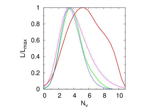
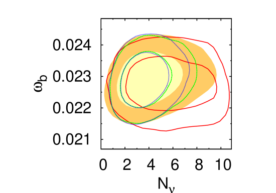
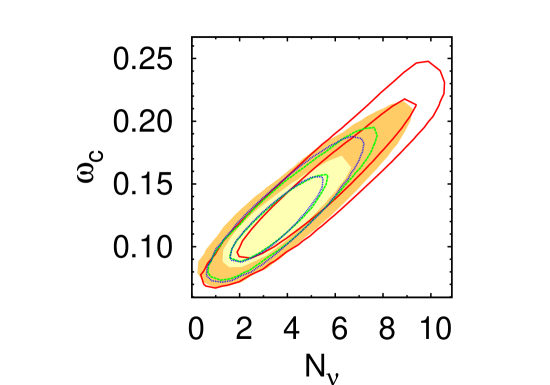
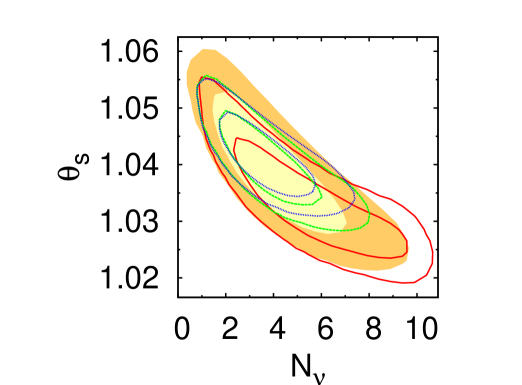
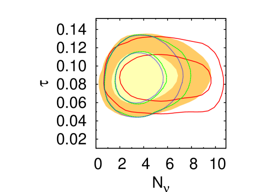
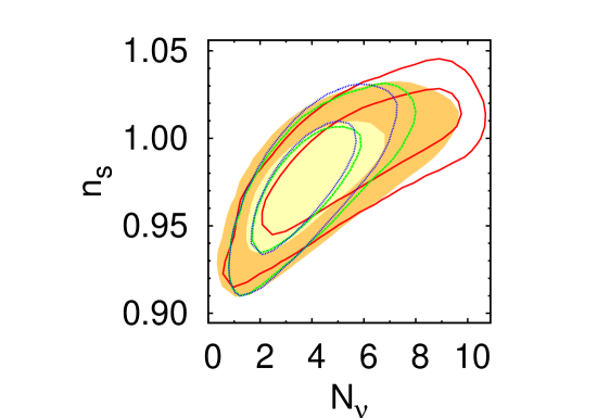
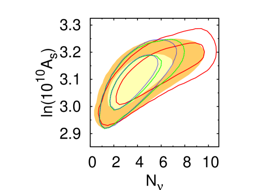
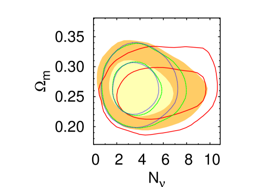
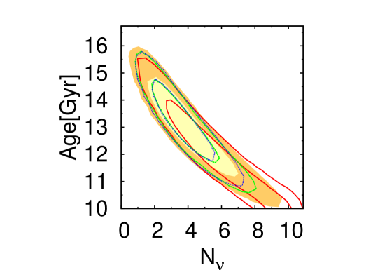
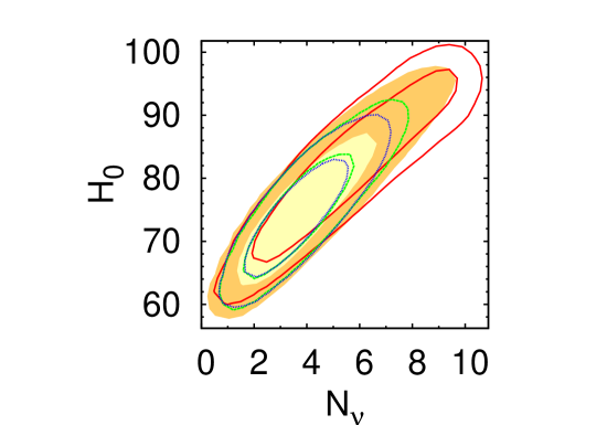
Now, we present our results in order. In Fig. 2, the posterior 1D distributions for are shown for the analysis with WMAP5 alone and WMAP5+ACBAR+BOOMERANG+CBI (CMB all). The former is shown by a red solid line. For the latter case, the results for different assumptions on are depicted: being fixed as (green dashed line), determined from the BBN relation (blue dotted line) and being treated as a free parameter (magenta dot-dashed line). Corresponding constraints on are summarized in Table 1. We also show 2D contours of 68% and 95% C.L. in the planes of v.s. several other cosmological parameters in Fig. 3. Table 2 summarizes the derived constraints on these parameters.
As seen from Fig. 2, the likelihood for from WMAP alone has irregular shape, far from Gaussian. It has the maximum around , declines slowly as increases and drop abruptly at . The abrupt cut can be traced to the prior on the cosmic age which is implicitly assumed as in the analysis. In particular, the lower limit makes the cut (see Fig 3). We can regard this prior to be very conservative on the observational ground since it is far looser than the astrophysical lower bound of the cosmic age e.g. (95% C.L.) from the age estimates of globular clusters [56]. Moreover, we should include such prior from the practical reason. As can be seen by the relatively slow decline of the likelihood for or the elongated contours in Fig 3, the degeneracy is so severe that we cannot produce MCMC chains which are well converged within a reasonable time. Although we can formally calculate a constraint using this data as shown in Table 1, since the likelihood is so irregular, we would conclude that it is not meaningful to constrain from WMAP5 alone.
However, it may be instructive to understand how the degeneracies arise in the WMAP-alone analysis. As clearly shown in Fig. 3, most notably degenerates with and (or ). There are also some degeneracies with and but not as severe as or . These degeneracies are understood as follows. First, to produce the same amount of the early ISW effect, has to be increased as increases. It roughly scales as to make the matter-radiation equality same. At the same time, under the flatness assumption, has to be preserved in order to have the same distance to the last scattering surface. Then, since , has to increase for larger . The slight enhancement in and can be attributed to their effects to cancel the suppression around the diffusion damping scales due to the increase in . A more quantitative argument based on the derivatives presented in the previous section may be useful. The degeneracy as regards the same matter-radiation equality is given by setting to be . This is equivalent to , which roughly gives the slope in the – plane in Fig 3. Using this relation with shows the – degeneracy. From Eq. (3), we obtain , which appear in the – contour in Fig 3. The – degeneracy is given by further requiring . Plugging and in Eq. (13) yields . This 5% increase in the best fit value of for is consistent with the – contour in Fig 3. Although WMAP has measured the CMB power spectrum very precisely, since it is just up to around the 2nd peak, the effects of are absorbed in the changes of , , and and we cannot constrain .
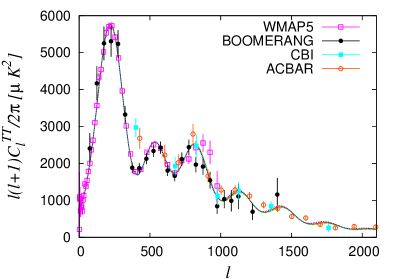
For a visual illustration of the degeneracy, in Fig. 4, we show CMB power spectra for the case with (blue dotted line), (red solid line) and (green dashed line) with other cosmological parameters being chosen such that they give the degenerate spectra up to the 2nd/3rd peak. We can see that these curves coincide up to the 2nd peak but begin to separate around the 3rd or the higher peaks. On small scales, the change caused by cannot be fully canceled just by tuning other parameters. In particular, affects the spectrum in the whole scales; thus, even if the spectra is almost degenerate up to the 2nd peak by tuning the value of , it cannot cancel the damping on small scales.
| parameters | CMB all | CMB all | CMB all | WMAP5 |
|---|---|---|---|---|
| (: free) | (: BBN relation) | () | () | |
| — | — | |||
| Age[Gyr] | ||||
When we include the data at higher multipoles such as ACBAR, BOOMERANG and CBI, the likelihood functions now have a well-behaved peak close to Gaussian and we can obtain meaningful constraints. The bound on is at 95 % C.L. when is treated as a free parameter. At higher multipoles, the free streaming of neutrinos damps the spectrum, which cannot be compensated by above-mentioned parameters. Hence the degeneracy can be removed to some extent. That is the reason why we can have a severer constraint on by including the data on small scales. In fact, also suppresses the amplitude on small scales via diffusion damping (see Eqs. (11) and (12)); thus the constraint on slightly changes for different treatments of but the differences are very small as seen in Fig. 2 and Table 1. Since current CMB observations on small scales are not so precise, it does not make much difference how we treat . Imposing the BBN relation tightens the constraint to at 95 % C.L., but it is not so different from the -free case. Also, the limit does not differ much even if we set . Similarly, the estimates for the other cosmological parameters are not affected by the assumption on as shown in Table 2.
| No priors on | |||||||
| Mean | 68% | 95% | 68% | 95% | 68% | 95% | |
| 68% | 95% | 68% | 95% | 68% | 95% | ||
| CMB all | (3.046) | (3.046) | |||||
| (: free) | |||||||
| CMB all | — | ||||||
| (: BBN relation) | |||||||
| CMB all | (3.046) | (3.046) | |||||
| (: fixed) | |||||||
| Planck | (3.046) | (3.046) | |||||
| (: free) | |||||||
| Planck | — | ||||||
| (: BBN relation) | |||||||
| Planck | (3.046) | (3.046) | |||||
| (: fixed) | |||||||
Up to now, we have assumed no prior on . However, if we consider an extra radiation component such as sterile neutrinos and so on, the effective number of neutrino species just increases. In this case, cannot be less than the standard value of 3.046. Thus it may be appropriate to study adopting the prior to constrain a scenario with such an extra radiation component. We denote it as . With this prior, we obtain an upper bound on an extra radiation component as (or ) at 95 % C.L. when is taken as a free parameter and improve to be (or ) at 95 % C.L. when the BBN relation is assumed. Notice that these limits are weaker than those with no priors on , which are () and (), respectively. This somewhat peculiar fact stems from the shape of the likelihood shown in Fig. 2, which is not symmetric with respect to . Since the differences due to the prior are not negligible, caution is needed when we use these constraints regarding the prior on .
Even when we limit ourselves to the case with three active neutrino species, a deviation from the standard value of is possible. In a scenario with low (MeV scale) reheating temperature, can be less than 3.046. In this case, only takes the value less than the standard one. Thus it may be interesting to investigate a constraint on assuming . As regards the treatment of , we do not consider the case with adopting the BBN relation here because, in a scenario with MeV reheating temperature, should be calculated taking into account the non-thermal neutrino distribution functions and oscillation effects [3, 4, 5, 6]. These effects drive to increase as decreases contrary to the usual case where just represents a measure of the expansion rate. (This is why we are not showing constraints for the prior with the BBN relation in Table 3.) Since taking into account this effect is beyond the scope of this paper, we show the constraint for the case with being varied freely, which can be considered as the conservative one for the prior . We obtained constraints and at 95% C.L. for the cases with being fixed as and being assumed as a free parameter, respectively. For a scenario with MeV scale reheating temperature, these limits are translated into the lower bound on the reheating temperature as MeV [6].
Finally, we investigate a future constraint on cosmological parameters paying particular attention to and its effects on constraints on other parameters. We use the data expected from the future Planck experiment and make a MCMC analysis following the method in Ref. [57]. As for the specification of Planck, we adopt the following parameters for the instrument. For the frequency channels of , 143 and 217 GHz, the width of the beam and the sensitivities per pixel for temperature and polarization are adopted as and , respectively. Other frequency channels are assumed to be used to remove foregrounds. We make use of the data up to in order that our results will not be affected by the SZ effect and the marginalization over is not performed. These setups for the Planck forecast are similar to the recent works performed in Refs. [51, 26, 30], but explored parameter spaces are different. We make a simple extension by adding and to the standard 6 dimensional parameter space, but theirs include neutrino masses and/or lepton asymmetry. When one would like to check the constraint on an extra radiation component in a simple scenario, one can refer our results here. However, when some other particular setups are considered such as a scenario with large lepton asymmetry and massive neutrinos, the above mentioned references should be consulted.
Our results are summarized in Tables 3 and 4. As seen from the Table 3, the constraint is most stringent when the BBN relation is adopted, and in this case, we obtained a future constraint as at 95 % C.L. Another point which should be noted is that fixing of can bias the determination of some other cosmological parameters such as and , which was already pointed out in Refs. [51, 52]. However, when we vary the value of , the effect of fixing of is partly cancelled by the change in . In fact, this in turn results in biases of other cosmological parameters such as and which are strongly correlated with . Therefore, should be carefully treated in investigating cosmological constraints with future CMB data.
| Planck | Planck | Planck | |
| parameters | (: free) | (: BBN relation) | () |
| — | |||
| Age[Gyr] | |||
We would like in the end to comment on how our discussion so far can be affected by theoretical uncertainties in the recombination process [58, 60, 66, 59, 61, 62, 63, 64, 65]. Since the change of can influence the recombination process, its uncertainties might affect the cosmological parameter determination in some way. Thus it may be worth mentioning here on the effects. For this purpose, we proceed with the same analysis as have been done in Ref. [52] but varying here. Two parameters and , which represent the uncertainties in the recombination modeling, are included among other free parameters. (See Ref. [52] and references therein for more details). We impose top-hat priors, and , which are very conservative ones, to take into account the uncertainties in the recombination theory. We made the analyses for the two cases where is given from the BBN relation and is treated as a free parameter. In both cases, we found that the constraints on other cosmological parameters including are scarcely affected even by very conservative prior on and . The mean values are unchanged and errors increase only very slightly (no more than 10% for any parameters other than and ). Therefore we can say that the uncertainties parametrized with and do not change much our results of the Planck forecast discussed above. However, we would need more understanding of uncertainties in the recombination theory for the precise determination of cosmological parameters in future CMB surveys.
4 Summary
We discussed the issue of probing the effective number of neutrino species from CMB data alone. Although a constraint on has been investigated by many authors, in most analyses, some combinations of data set such as CMB+LSS, CMB+, CMB+LSS+ have been used to constrain . This is partly because has severe degeneracies in WMAP with some other cosmological parameters such as and ; thus can be more constrained by combining some data sets. However, when we combine data from LSS, some subtleties can arise: a constraint from LSS data depends on how we treat non-linear corrections/bias. Furthermore, different galaxy data lead to slightly different constraints on . In addition, as for the Hubble prior, the prior usually adopted is which is from the result of Freedman et al [31]. However, another group has reported somewhat different value as [32]. Since different priors on the Hubble constant can give different results, in this respect, the constraint obtained by assuming some prior on should be regarded taking into account the above uncertainty. Taking these issues into consideration, it may be interesting to study a constraint on removing such subtleties, which can be done by using CMB data alone.
In this paper, first we discussed the effects of on CMB and the issues of degeneracies with some other cosmological parameters. Phenomenological descriptions of its effects on the heights and the positions of acoustic peaks were also given. Then, in section 3, a constraint on was studied by using CMB data alone. We made use of the data from WMAP5, ACBAR, BOOMERANG and CBI. As discussed there, although WMAP measurement is very accurate, its precision is limited up to the 2nd peak/3rd peak. We have explicitly shown that the information up to the 2nd/3rd peak is not enough to constrain severely. This was demonstrated by making the analysis with WMAP data alone, in which a sensible constraint cannot be obtained. However, if we include the data on small scales, the degeneracies of with some other cosmological parameters can be removed to some extent; then a stronger constraint can be obtained. In fact, on small scales, the amplitude is suppressed due to the free streaming effect by increasing , which is similar to the effects of through the diffusion damping. Thus we have studied the constraint on assuming different priors on : adopting the BBN relation to derive for given and , assuming as a free parameter and usual fixing of . Depending on the prior, the constraint slightly changes. We obtained the 95 % limits as for the case with being free, for being fixed as and when the BBN relation being adopted. It should be noted that these constraints are comparable to that obtained using CMB+LSS in previous works.
One of the main purposes of constraining the effective number of neutrino species using cosmological data is to check the standard value of independently from particle physics experiments. Thus we primarily focus on the analysis with no prior on . However, from the viewpoint of constraining extra radiation which may be motivated from some particle physics models, a constraint obtained by assuming the prior may be interesting since an extra radiation always increases the value of . In this respect, we also made an analysis adopting this prior and obtained the constraint on the effective number of neutrino as and for the cases where the BBN relation is adopted and is treated as a free parameter.
On the other hand, in a scenario with low-reheating temperature, the effective number of neutrino species can be reduced. In this case, another prior may be motivated to be assumed for a simple scenario of low-reheating temperature with three relativistic neutrino species. In this regard, we have also studied the case with the prior and obtained the constraints as for the cases with being assumed as a free parameter. This can be translated into the lower bound on the reheating temperature as MeV.
We have also discussed a future constraint on using the expected data from Planck experiment. It was shown that the attainable constraint on from Planck is at 95% C.L. when the BBN relation is adopted for , which is most stringent compared to the other cases. Since Planck experiment can probe CMB down to smaller scales than WMAP, Planck alone can give a stringent constraint on .
The interplay between particle physics and cosmology is now becoming more important in the era of precision cosmology. One of such examples is the number of neutrino species, which was investigated in this paper. In light of upcoming more precise observations of cosmology, research of this kind will bring us fruitful insight for particle physics and cosmology.
Acknowledgments: This work is supported in part by the Japan Society for the Promotion of Science (K.I. and T.S.), the Sumitomo Foundation (T.T.), and the Grant-in-Aid for Scientific Research from the Ministry of Education, Science, Sports, and Culture of Japan, No. 18840010 (K.I.) and No. 19740145 (T.T.).
References
- [1] W. M. Yao et al. [Particle Data Group], J. Phys. G 33 (2006) 1.
- [2] A. D. Dolgov, Phys. Rept. 370, 333 (2002) [arXiv:hep-ph/0202122].
- [3] M. Kawasaki, K. Kohri and N. Sugiyama, Phys. Rev. Lett. 82, 4168 (1999) [arXiv:astro-ph/9811437].
- [4] M. Kawasaki, K. Kohri and N. Sugiyama, Phys. Rev. D 62, 023506 (2000) [arXiv:astro-ph/0002127].
- [5] S. Hannestad, Phys. Rev. D 70, 043506 (2004) [arXiv:astro-ph/0403291].
- [6] K. Ichikawa, M. Kawasaki and F. Takahashi, Phys. Rev. D 72, 043522 (2005) [arXiv:astro-ph/0505395].
- [7] J. P. Kneller, R. J. Scherrer, G. Steigman and T. P. Walker, Phys. Rev. D 64, 123506 (2001) [arXiv:astro-ph/0101386].
- [8] S. Hannestad, Phys. Rev. D 64, 083002 (2001) [arXiv:astro-ph/0105220].
- [9] R. Bowen, S. H. Hansen, A. Melchiorri, J. Silk and R. Trotta, Mon. Not. Roy. Astron. Soc. 334, 760 (2002) [arXiv:astro-ph/0110636].
- [10] P. Crotty, J. Lesgourgues and S. Pastor, Phys. Rev. D 67, 123005 (2003) [arXiv:astro-ph/0302337].
- [11] E. Pierpaoli, Mon. Not. Roy. Astron. Soc. 342, L63 (2003) [arXiv:astro-ph/0302465].
- [12] S. Hannestad, JCAP 0305, 004 (2003) [arXiv:astro-ph/0303076].
- [13] V. Barger, J. P. Kneller, H. S. Lee, D. Marfatia and G. Steigman, Phys. Lett. B 566, 8 (2003) [arXiv:hep-ph/0305075].
- [14] P. Crotty, J. Lesgourgues and S. Pastor, Phys. Rev. D 69, 123007 (2004) [arXiv:hep-ph/0402049].
- [15] S. Hannestad, JCAP 0601, 001 (2006) [arXiv:astro-ph/0510582].
- [16] D. N. Spergel et al. [WMAP Collaboration], Astrophys. J. Suppl. 170, 377 (2007) [arXiv:astro-ph/0603449].
- [17] U. Seljak, A. Slosar and P. McDonald, JCAP 0610, 014 (2006) [arXiv:astro-ph/0604335].
- [18] S. Hannestad and G. G. Raffelt, JCAP 0611, 016 (2006) [arXiv:astro-ph/0607101].
- [19] M. Cirelli and A. Strumia, JCAP 0612, 013 (2006) [arXiv:astro-ph/0607086].
- [20] K. Ichikawa, M. Kawasaki and F. Takahashi, JCAP 0705, 007 (2007) [arXiv:astro-ph/0611784].
- [21] G. Mangano, A. Melchiorri, O. Mena, G. Miele and A. Slosar, JCAP 0703, 006 (2007) [arXiv:astro-ph/0612150].
- [22] A. Friedland, K. M. Zurek and S. Bashinsky, arXiv:0704.3271 [astro-ph].
- [23] J. Hamann, S. Hannestad, G. G. Raffelt and Y. Y. Y. Wong, JCAP 0708, 021 (2007) [arXiv:0705.0440 [astro-ph]].
- [24] K. Ichikawa, arXiv:0706.3465 [astro-ph].
- [25] F. de Bernardis, A. Melchiorri, L. Verde and R. Jimenez, JCAP 0803, 020 (2008) [arXiv:0707.4170 [astro-ph]].
- [26] L. A. Popa and A. Vasile, arXiv:0801.3928 [astro-ph].
- [27] E. Komatsu et al. [WMAP Collaboration], arXiv:0803.0547 [astro-ph].
- [28] J. Dunkley et al. [WMAP Collaboration], arXiv:0803.0586 [astro-ph].
- [29] V. Simha and G. Steigman, JCAP 0806, 016 (2008) [arXiv:0803.3465 [astro-ph]].
- [30] L. A. Popa and A. Vasile, JCAP 0806, 028 (2008) [arXiv:0804.2971 [astro-ph]].
- [31] W. L. Freedman et al. [HST Collaboration], Astrophys. J. 553, 47 (2001) [arXiv:astro-ph/0012376].
- [32] A. Sandage, G. A. Tammann, A. Saha, B. Reindl, F. D. Macchetto and N. Panagia, Astrophys. J. 653, 843 (2006) [arXiv:astro-ph/0603647].
- [33] S. Bashinsky and U. Seljak, Phys. Rev. D 69, 083002 (2004) [arXiv:astro-ph/0310198].
- [34] C. L. Reichardt et al., arXiv:0801.1491 [astro-ph].
- [35] G. Mangano, G. Miele, S. Pastor, T. Pinto, O. Pisanti and P. D. Serpico, Nucl. Phys. B 729, 221 (2005) [arXiv:hep-ph/0506164].
- [36] W. Hu, M. Fukugita, M. Zaldarriaga and M. Tegmark, Astrophys. J. 549, 669 (2001) [arXiv:astro-ph/0006436].
- [37] G. Hinshaw et al. [WMAP Collaboration], arXiv:0803.0732 [astro-ph].
- [38] R. S. Hill et al. [WMAP Collaboration], arXiv:0803.0570 [astro-ph].
- [39] M. R. Nolta et al. [WMAP Collaboration], arXiv:0803.0593 [astro-ph].
- [40] W. C. Jones et al., Astrophys. J. 647, 823 (2006) [arXiv:astro-ph/0507494].
- [41] F. Piacentini et al., Astrophys. J. 647, 833 (2006) [arXiv:astro-ph/0507507].
- [42] T. E. Montroy et al., Astrophys. J. 647, 813 (2006) [arXiv:astro-ph/0507514].
- [43] J. L. Sievers et al., arXiv:astro-ph/0509203.
- [44] A. Lewis and S. Bridle, Phys. Rev. D 66, 103511 (2002) [arXiv:astro-ph/0205436].
- [45] A. Kosowsky, M. Milosavljevic and R. Jimenez, Phys. Rev. D 66, 063007 (2002) [arXiv:astro-ph/0206014].
- [46] E. Komatsu and U. Seljak, Mon. Not. Roy. Astron. Soc. 336, 1256 (2002) [arXiv:astro-ph/0205468].
- [47] L. H. Kawano, FERMILAB-Pub-92/04-A (1992).
- [48] C. Angulo et al., Nucl. Phys. A. 656, 3 (1999).
- [49] G. Huey, R. H. Cyburt and B. D. Wandelt, Phys. Rev. D 69, 103503 (2004) [arXiv:astro-ph/0307080].
- [50] K. Ichikawa and T. Takahashi, Phys. Rev. D 73, 063528 (2006) [arXiv:astro-ph/0601099].
- [51] J. Hamann, J. Lesgourgues and G. Mangano, JCAP 0803, 004 (2008) [arXiv:0712.2826 [astro-ph]].
- [52] K. Ichikawa, T. Sekiguchi and T. Takahashi, Phys. Rev. D 78, 043509 (2008) [arXiv:0712.4327 [astro-ph]].
- [53] P. D. Serpico, S. Esposito, F. Iocco, G. Mangano, G. Miele and O. Pisanti, JCAP 0412, 010 (2004) [arXiv:astro-ph/0408076].
- [54] K. Ichikawa, M. Kawasaki and F. Takahashi, Phys. Lett. B 597, 1 (2004) [arXiv:astro-ph/0402522].
- [55] K. Ichikawa, M. Kawasaki, K. Nakayama, M. Senami and F. Takahashi, JCAP 0705, 008 (2007) [arXiv:hep-ph/0703034].
- [56] L. M. Krauss and B. Chaboyer, Science 299, 65 (2003).
- [57] L. Perotto, J. Lesgourgues, S. Hannestad, H. Tu and Y. Y. Y. Wong, JCAP 0610, 013 (2006) [arXiv:astro-ph/0606227].
- [58] S. Seager, D. D. Sasselov and D. Scott, Astrophys. J. Lett. 523, L1 (1999) arXiv:astro-ph/9909275.
- [59] J. Chluba and R. A. Sunyaev, Astron. Astrophys. 446, 39 (2006) [arXiv:astro-ph/0508144].
- [60] A. Lewis, J. Weller and R. Battye, Mon. Not. Roy. Astron. Soc. 373, 561 (2006) [arXiv:astro-ph/0606552].
- [61] J. Chluba, J. A. Rubino-Martin and R. A. Sunyaev, Mon. Not. Roy. Astron. Soc. 374, 1310 (2007) [arXiv:astro-ph/0608242].
- [62] J. Chluba and R. A. Sunyaev, arXiv:astro-ph/0702531.
- [63] E. R. Switzer and C. M. Hirata, Phys. Rev. D 77, 083006 (2008) [arXiv:astro-ph/0702143].
- [64] C. M. Hirata and E. R. Switzer, Phys. Rev. D 77, 083007 (2008) [arXiv:astro-ph/0702144].
- [65] E. R. Switzer and C. M. Hirata, Phys. Rev. D 77, 083008 (2008) [arXiv:astro-ph/0702145].
- [66] W. Y. Wong, A. Moss and D. Scott, arXiv:0711.1357 [astro-ph].