On deriving p-mode parameters for inclined solar-like stars

Abstract

Context. Thanks to their high quality, new and upcoming asteroseismic observations – with CoRoT, Kepler, and from the ground… – can benefit from the experience gained with helioseismology.

Aims. We focus in this paper on solar-like oscillations, for which the inclination of the rotation axis is unknown. We present a theoretical study of the errors of p-mode parameters determined by means of a maximum-likelihood estimator, and we also analyze correlations and biases.

Methods. We have used different, complementary approaches: we have performed either semi-analytical computation of the Hessian matrix, fitting of single mean profiles, or Monte Carlo simulations.

Results. We give first analytical approximations for the errors of frequency, inclination and rotational splitting. The determination of the inclination is very challenging for the common case of slow rotators (like the Sun), making difficult the determination of a reliable rotational splitting. Moreover, due to the numerous correlations, biases – more or less significant – can appear in the determination of various parameters in the case of bad inclination fittings, especially when a locking at 90° occurs. This issue concerning inclination locking is also discussed. Nevertheless, the central frequency and some derived parameters such as the total power of the mode are free of such biases.

1 Introduction

A new era of the asteroseismic observations is now opening with CoRoT (Baglin et al. 2006), and will be pursued in the near future with Kepler (Borucki et al. 2007). As these missions will provide long and uninterrupted time series of intensity measurements, the quality of these data will become closer to those of helioseismology, although with a higher level of noise expected. In such a context, asteroseismology can fruitfully inherit the methods and techniques developed for helioseismology, especially for so-called ‘Sun-as-a-star’ observations, such as those provided by the space instruments GOLF (Gabriel et al. 1995) or VIRGO (Fröhlich et al. 1995) onboard the SoHO spacecraft or by ground-based networks like BiSON (Chaplin et al. 1996).

We discuss in this paper the usual way to extract information on stochastically excited acoustic (p) modes in helioseismology. P modes can be described by several parameters (frequency, lifetime, amplitude… ) which can be derived by fitting the stellar oscillation power spectrum with a maximum-likelihood estimation. As for any measurement, we need to associate with each derived parameter a correct error bar, that is essential to estimate the significance of the measurement and thus to be able to do a reasonable interpretation. We present here theoretical results on the derivation of errors of p-mode parameters and their correlations. This work generalizes some results already known in helioseismology (Libbrecht 1992; Toutain & Appourchaux 1994) by adding the inclination of the stellar rotation axis, $i$, as an extra free parameter.

Fitting methods with a free inclination angle have first been analyzed by Gizon & Solanki (2003), then by Ballot et al. (2006). In the present paper, we develop a more complete version of a preliminary work (Ballot et al. 2008) on analytical formulations of error bars for several parameters, and we have completed it with an analysis of correlations and biases. We have especially considered here the very common cases of slow rotators, for which the mode linewidth is greater than (or similar to) the rotational splitting, giving rise to a blending of multiplet components.

In § 2, we define the model assumed for p modes and the fitting method. Section 3 deals with error bars obtained for the mode frequencies, the splittings and the inclination. The correlation between different parameters is studied in § 4 and some biases of the method are analyzed in § 5. Finally we briefly discuss the locking of the inclination determination at 90° which often appears during fitting (§ 6).

2 Models and Methods

2.1 Modeling the power spectrum

Stellar acoustic eigenmodes are characterized by their degree $l$, their azimuthal order $m$ and their radial order $n$. In this study, we treat p modes according to the solar paradigm. Modes are modelled as stochastically excited and intrinsically damped harmonic oscillators (see Kumar et al. 1988). In that case, the power spectrum – obtained by computing the discrete Fourier transform of an evenly sampled timeseries – of such modes is distributed around a mean Lorentzian profile with an exponential probability distribution. A Lorentzian profile is defined as

$$L(A,\nu_{0},\Gamma;\nu)=\frac{A}{1+\left(\frac{\nu-\nu_{0}}{\Gamma/2}\right)^{2}},$$ (1)

where $A$ is the mode height, $\Gamma=(\pi\tau)^{-1}$ the mode linewidth, linked to the damping time $\tau$, and $\nu_{0}$ the mode frequency. For our examples we have considered the value $\Gamma=1\>\mathrm{\mu Hz}$ in the whole study, that corresponds to a lifetime around 3–4 days. This is a typical observed value of solar p-mode linewidths in a broad range around 2500–3000$\>\mathrm{\mu Hz}$ (e.g. García et al. 2004).

Since stellar rotation lifts the azimuthal degeneracy of eigenmodes, the power spectrum of a mode with a degree $l$ is a multiplet with $2l+1$ components. Extrapolating from the solar case, we assume equipartition of energy between the components in a multiplet, and we define a multiplet as a symmetric profile:

$$M_{l}(A,\nu_{0},\Gamma,\nu_{s},i;\nu)=\sum_{m=-l}^{l}a_{l,m}(i)L(A,\nu_{0}+m\nu_{s},\Gamma;\nu),$$ (2)

where $\nu_{s}$ is the rotational splitting and the inclination $i$ is the angle between the rotation axis and the line of sight.

We have used here the approximation of Ledoux (1951) for an uniform rotation: the frequency shift of the $m$-component relative to the central one is $\nu_{m}-\nu_{0}=m\nu_{s}$; moreover, we consider $\nu_{s}\approx\Omega/(2\pi)$, that is the asymptotic regime at high order $n$ ($\Omega$ is the stellar rotation rate). This approximation is valid when rotation is sufficiently slow and there is neither a strong differential rotation nor a strong magnetic activity.

Next, the inclination acts only on $a_{l,m}(i)$, the amplitude ratios of components inside a multiplet, which satisfies the relationship $\sum_{m}a_{l,m}=1$. Thus the total power of a multiplet is always $P=\frac{\pi}{2}A\Gamma$. The amplitude ratios are written

$$a_{l,m}(i)=\frac{|l-m|!}{|l+m|!}(P_{l,m}(\cos i))^{2}$$ (3)

where $P_{l,m}$ are the associated Legendre functions (see Gizon & Solanki 2003). To derive this expression, when the flux is integrated over the full stellar disc, we need to assume that the weighting function, which gives the contribution of a point on the disc to the integral, is a function of the distance to the disc center only. This is correct for intensity measurements, because the weighting function is mainly linked to the limb-darkening. However for velocity measurements, we can observe departures from this law, since the rotation of the star induces an asymmetry in the velocity field.

Last, we have also assumed that a mode is not correlated with any other modes or with the convective background noise. Doing so we neglect in the present study any possible asymmetry of the Lorentzian profiles (Nigam et al. 1998). According to what we have learned from helioseismology, neglecting asymmetries could introduce systematic errors (i.e. biases) in mode frequency determination. These errors are of the order of 0.1$\>\mathrm{\mu Hz}$ in the solar case (Toutain et al. 1997). This is on par with the statistical error (i.e. the standard deviation) of the frequency for time series of several months. For longer time series (few years), the asymmetry should be included in the fitted profiles to avoid systematic errors in mode frequencies.

To summarize, we have considered that the star is observed in intensity, that the mode excitation mechanisms are close to those of the Sun, and that the star does not rotate too rapidly (a few times the solar rate).

2.2 Maximum-likelihood estimator

P-mode parameters are fitted with a classical maximum-likelihood estimation technique and the associated error and correlation are estimated by inverting the Hessian matrix (Toutain & Appourchaux 1994; Appourchaux et al. 1998). In practice, instead of maximizing the likelihood, we minimize the negative logarithm of the likelihood function, which yields for a random exponential noise:

$$\ell(\@vec{\lambda})=-\ln{\cal L}(\@vec{\lambda})=\sum_{k=1}^{N}\ln S(\@vec{\lambda};\nu_{k})+\frac{S_{k}}{S(\@vec{\lambda};\nu_{k})}$$ (4)

where $S$ is the model of the spectrum measured $\{S_{k}\}_{k=1,N}$ at frequencies $\{\nu_{k}\}$, and $\@vec{\lambda}=(\lambda_{1},\dots,\lambda_{p})$ is the set of $p$ parameters to be adjusted. We denote hereafter $\tilde{\lambda}_{j}$ an estimation of $\lambda_{j}$.

As the observed intensity fluctuations are integrated over the whole stellar disc, only low-degree modes are visible. A quick estimation of their visibility indicates that we will mainly be able to detect only modes with $l\leq 2$ and perhaps a few $l=3$ modes.

We have therefore considered the following fitting cases: 1) we fit a mode $l=1$ alone; $S$ is described by 6 parameters: $A$, $\nu_{0}$, $\Gamma$, $i$, $\nu_{s}$, and a additive background $B$ assumed to be flat within the fitting window. In practice, we fit the logarithm of some of the parameters: $a=\ln A$, $\gamma=\ln\Gamma$ and $b=\ln B$. 2) We fit a pair of modes $l=0$ and 2; assuming a common linewidth for both modes $S$ is described by 8 parameters; 3) We fit a sequence of modes $l=0$, 2 and 1; $S$ is described by 11 parameters, assuming the splitting is the same for the consecutive $l=1$ and 2 modes.

The standard deviations (error bars) $\sigma_{j}$ associated with $\lambda_{j}$ are estimated with the covariance matrix $\mathbf{C}$, computed by inverting the Hessian matrix $\mathbf{H}$ ($\mathbf{C}=\mathbf{H}^{-1}$). The diagonal elements of $\mathbf{C}$ give the errors $c_{jj}=\sigma_{j}^{2}$, while the non-diagonal elements give the covariances $c_{ij}=\sigma_{ij}=\rho_{ij}\sigma_{i}\sigma_{j}$ ($\rho_{ij}$ are the correlation coefficients).

The terms of the Hessian are:

$$h_{ij}=\left.\frac{\partial^{2}\ell(\@vec{\lambda})}{\partial\lambda_{i}\partial\lambda_{j}}\right|_{\@vec{\lambda}=\@vec{\tilde{\lambda}}}.$$ (5)

Following Libbrecht (1992) and Toutain & Appourchaux (1994), we define a theoretical Hessian corresponding to the average of a large number of realizations:

$$h_{ij}=\sum_{k=1}^{N}\frac{1}{S^{2}(\@vec{\lambda};\nu_{k})}\frac{\partial S}{\partial\lambda_{i}}\frac{\partial S}{\partial\lambda_{j}}.$$ (6)

If the frequency bin is much smaller than the mode linewidth, we can approximate the Hessian by the integral:

$$\ h_{ij}=T\int_{-\infty}^{+\infty}\frac{1}{S^{2}(\@vec{\lambda};\nu)}\frac{\partial S}{\partial\lambda_{i}}\frac{\partial S}{\partial\lambda_{j}}d\nu,$$ (7)

where $T$ is the observation duration.

In the next sections, results concerning errors, correlations and biases are obtained with semi-analytical computations of Eqs. 6 and 7, by fitting the mode profile model as in Toutain et al. (2005), or with Monte Carlo simulations.

3 Theoretical error bars

3.1 Error of the central frequency $\nu_{0}$

Figure 1: Frequency error computed with Eq. (9) for modes $l=1$ (left) and $l=2$ (right) as a function of the angle $i$, for different reduced splittings $x_{s}=$ 0.4 (dots), 0.8 (solid line), 1.6 (dashes), 2.4 (dot-dash), 4.0 (dot-dot-dot-dash), 8.0 (long dashes); that corresponds, for $\Gamma=1\>\mu$Hz, to $\Omega=$0.5, 1, 2, 3, 5, 10$\>\Omega_{\odot}$. Thick long dashes indicate the limit when $x_{s}\gg 1$, computed with Eq. (13). Here $\beta=1/20$ and $T=6\>$months.

We generalize in this section the results of Libbrecht (1992) and Toutain & Appourchaux (1994), inferred for $l=0$ and for multiplets in the solar configuration ($i=90\degr$).

Considering an isolated multiplet $S=B+M_{l}$, we can easily verify that $h_{\nu_{0},j}(=h_{j,\nu_{0}})=0$ except for $\lambda_{j}=\nu_{0}$. Since $S$ is even in the variable $\nu-\nu_{0}$, the derivatives $\partial_{\nu_{0}}S=-\partial_{\nu}S$ are odd. However we can verify that $\partial_{\lambda_{j}}S$ is even relative to the variable $\nu-\nu_{0}$ for all of the other parameters $\lambda_{j}=B,A,\Gamma,\nu_{s}$ and $i$. This is easy to demonstrate by noting that any modification of one or several of these parameters preserves the symmetry of the profile with respect to $\nu-\nu_{0}$. With the same argument, we easily demonstrate that, after any variable change $\lambda_{j}=f(B,A,\Gamma,\nu_{s},i)$, $\partial_{\lambda_{j}}S$ is still even. Thus, in Eq. 7, the function under the integral is odd, and the integral vanishes. We deduce that

$$\sigma^{2}_{\nu_{0}}=h_{\nu_{0}\nu_{0}}^{-1}\qquad\mbox{and}\qquad\sigma_{\nu_{0}j}=0\quad\forall\lambda_{j}\neq\nu_{0}.$$ (8)

The lack of correlation of $\nu_{0}$ with all other parameter is well established in Monte Carlo (MC) simulations. When a pair (for instance $l=0$ and 2) is fitted, this is still correct while the modes are well separated: given $\lambda_{j}^{(0)}$ and $\lambda_{k}^{(2)}$ two parameters of the considered $l=0$ and $l=2$ modes, then $\partial_{\lambda_{j}^{(0)}}S\partial_{\lambda_{k}^{(2)}}S\approx 0\ \forall\nu$, since either $\partial_{\lambda_{j}^{(0)}}S$ or $\partial_{\lambda_{k}^{(2)}}S$ vanishes, as modes are sufficiently far apart. However, when modes are blended, crosstalk can occur and the central frequency can become correlated with other parameters, especially with the central frequency of the neighbor mode. Moreover, if the mode profiles are not symmetric (asymmetries in the Lorentzian or in the splittings), the mode frequencies can also become correlated with the others parameters, but a priori we expect negligibly small effects.

From Eq. 7, we derive the error for $\nu_{0}$:

$$\sigma^{2}_{\nu_{0}}=\frac{1}{4\pi}\frac{\Gamma}{T}f_{l}(\beta,x_{s},i),$$ (9)

with $\beta=B/A$ the noise-to-signal ratio and $x_{s}=2\nu_{s}/\Gamma$ the reduced splitting. For $l=0$, we find the formula of Libbrecht (1992):

$$f_{0}(\beta\mbox{ only})=\sqrt{\beta+1}\left(\sqrt{\beta+1}+\sqrt{\beta}\right)^{3}.$$ (10)

For $l>0$, the simplest form of $f_{l}$ is its integral form:

$$f_{l}(\beta,x_{s},i)=\frac{\pi}{4}\left[\int_{0}^{+\infty}\left[\frac{\sum_{m}a_{l,m}(i)(x+mx_{s})L_{r}^{2}(x+mx_{s})}{\beta+\sum_{m}a_{l,m}(i)L_{r}(x+mx_{s})}\right]^{2}dx\right]^{-1}$$ (11)

where

$$L_{r}(x)=\frac{1}{1+x^{2}}$$ (12)

is the reduced Lorentzian.

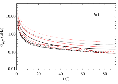
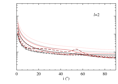
Figure 1 shows the evolution of $\sigma_{\nu_{0}}$ with $i$ and $x_{s}$ for $l=$1 and 2 modes. As expected, $f_{l}(\beta,x_{s},i)$ approches $f_{0}(\beta)$, as $i$ or $x_{s}$ approches zero. We can also notice that, when $x_{s}\ll 1$, the splitting acts as an extra width, increasing the error for $\nu_{0}$. Furthermore we clearly see that, depending of the values of $i$ and $x_{s}$, the error bars for $\nu_{0}$ can vary within a factor of 2. When $x_{s}\gg 1$, i.e. for large rotation rates, the components are well-separated, the fitting gives exactly the same result as when each $m$-component is independently fitted and the central frequency is computed with a weighted average: $\nu_{0}=\sum_{m}{\nu_{m}}{\sigma_{\nu_{m}}^{-2}}/\sum_{m}{\sigma_{\nu_{m}}^{-2}}$. The associated error is then

$$\sigma^{-2}_{\nu_{0}}=\sum_{m=-l}^{l}\sigma^{-2}_{\nu_{m}}=\frac{4\pi T}{\Gamma}\sum_{m=-l}^{l}\left[f_{0}\left(\frac{\beta}{a_{l,m}(i)}\right)\right]^{-1}.$$ (13)

This value, plotted in Fig. 1 as a thick dashed line, gives the lowest limit for the error at a given angle, linewidth and S/N ratio.

3.2 Error of the angle $i$ and the splitting $\nu_{s}$

Figure 2: Error for the angle $i$, the splitting $\nu_{s}$, and the projected splitting $\nu_{s}^{*}$, as a function of $i$, for modes $l=1$ (left) and $l=2$ (right), for different values of $x_{s}$ (see caption of Fig. 1). Black lines show errors obtained with the simplified Hessian, thin red lines are obtained by inverting the full Hessian. Thick long dashes in the middle panels indicate the limit of the error on $\nu_{s}$ when $x_{s}\gg 1$, computed with Eq. (22). Here $\beta=1/20$ and $T=6\>$months.

We focus now on the error of the inclination and the splitting, or other related variables. Ballot et al. (2006) have used the pair of parameters $(i,\nu_{s}^{*})$ instead of $(i,\nu_{s})$, where $\nu_{s}^{*}=\nu_{s}\sin i$ is the projected splitting. The authors did not see any difference in the determination of $i$ using one set of variables or the other. We analytically derive this result here, and we study more generally what happens when we fit other sets of parameters, for instance $(\sin^{2}i,\nu_{s})$ as further mentioned in § 6.

Let us denote by $(p,q)$ a new pair of parameters such $i=f_{i}(p)$ and $\nu_{s}=f_{S}(p,q)$. We consider a simplified Hessian matrix 2$\times$2 with elements (see Eq. 6):

$$h_{i} = \sum\frac{1}{S^{2}}\left(\frac{\partial S}{\partial i}\right)^{2}$$ (14)

$$h_{s} = \sum\frac{1}{S^{2}}\left(\frac{\partial S}{\partial\nu_{s}}\right)^{2}$$ (15)

$$h_{is} = \sum\frac{1}{S^{2}}\frac{\partial S}{\partial\nu_{s}}\frac{\partial S}{\partial i}$$ (16)

The errors for $i$ and $\nu_{s}$ are

$$\sigma_{i}^{-2} = h_{i}-\frac{h_{is}^{2}}{h_{s}},$$ (17)

$$\sigma_{\nu_{s}}^{-2} = h_{s}-\frac{h_{is}^{2}}{h_{i}}.$$ (18)

We denote by $\mathbf{G}$ the simplified Hessian matrix for the new parameters. Its elements are $g_{p}$, $g_{q}$ and $g_{pq}$. Using rules of (partial) derivatives, we show that:

$$\sigma_{p}^{2}=\frac{g_{q}}{g_{p}g_{q}-g_{pq}^{2}}=\left|\frac{dp}{di}\right|^{2}\frac{h_{s}}{h_{i}h_{s}-h_{is}^{2}}=\left|\frac{dp}{di}\right|^{2}\sigma_{i}^{2},$$ (19)

and

$$\sigma_{q}=\left(\frac{\partial f_{S}}{\partial q}\frac{df_{i}}{dp}\right)^{-1}\sqrt{\frac{g_{p}}{h_{i}}}\sigma_{\nu_{s}}.$$ (20)

Specifically for $p=i$ and $q=\nu_{s}^{*}$, we find:

$$\sigma_{\nu_{s}^{*}}=\sigma_{\nu_{s}}\sin i\sqrt{1+\frac{\nu_{s}^{2}}{\tan^{2}i}\frac{h_{s}}{h_{i}}-2\frac{\nu_{s}}{\tan i}\frac{h_{is}}{h_{i}}}.$$ (21)

First we conclude that the error for $i$ does not depend on the choice made for the other variables: $\nu_{s}$, $\nu_{s}^{*}$, or another combination. MC simulations and all of our other tests confirm this. Second, using $\cos i$ or $\sin i$ does not modify the error: we retrieve natural relationships such as $\sigma_{\sin^{2}i}=|\sin 2i|\sigma_{i}$.

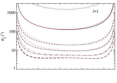
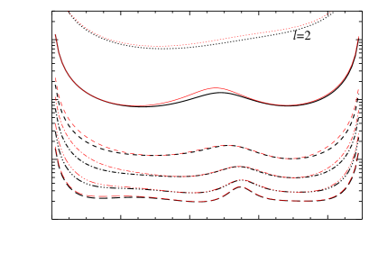
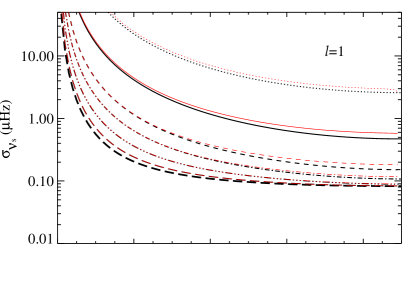
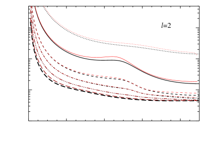
Figure 2 shows the errors we derive for the angle $i$, the splitting $\nu_{s}$ and the projected splitting $\nu_{s}^{*}$ for 6-month long observations. We compare the results from a simplified Hessian to those obtained by fitting directly the profile model (see method in Toutain et al. 2005). For the angle, both computations give very similar results. Estimated errors clearly demonstrate the difficulty in deriving a reliable determination of the angle $i$ from one single mode when the rotation is less than 2$\Omega_{\sun}$: the uncertainty covers almost the entire possible range. $l=2$ modes provide slightly better estimates of $i$ than $l=1$ modes because they have more components and the displacement of the $l=2$ modes is twice that of the $l=1$ modes. These error estimations are in agreement with those of Gizon & Solanki (2003), who have also numerically derived errors from the Hessian. Dividing by $\sqrt{8}$, the values of the errors in Figure 2 would give the corresponding errors for 4 years of observation (scales as the square root of the ratio of the observing times). Unless several modes are used to determine the inclination and the rotation, 4 years is still not sufficient to get enough accuracy when $\Omega\la\Omega_{\sun}$. However, if we measure 10 independent modes (for instance, 5 $l=1$ and 5 $l=2$), by averaging the results, we can expect to reduce the error to $\sim 15\degr$ for $\Omega=\Omega_{\sun}$.

Concerning the error for the splitting $\nu_{s}$, our simplified analysis also gives a result in good agreement with the complete numerical computation. We notice as well the dramatic increase of the errors when $\nu_{s}$ decreases. As previously done for the central frequency, we can also derive here the limit of the splitting error when $x_{s}\gg 1$ and that all of the components can be fitted independently. The resulting error for $\nu_{s}$ in this case is given by:

$$\sigma^{-2}_{\nu_{s}}=\sum_{m=-l}^{l}m^{2}\sigma^{-2}_{\nu_{m}}=\frac{8\pi T}{\Gamma}\sum_{m=1}^{l}m^{2}\left[f_{0}\left(\frac{\beta}{a_{l,m}(i)}\right)\right]^{-1}.$$ (22)

Interestingly enough it gives a lower bound for $\sigma_{\nu_{s}}$ for given $i$, $T$, $\Gamma$ and $\beta$.

The lower plots in Fig. 2 show the error of the projected splitting $\nu_{s}^{*}$. One sees that our simplified calculation is slightly more crude in this case. In this simplified approach, the correlations of $i$, $\nu_{s}$ and $\nu_{s}^{*}$ with the other parameters are neglected. They are actually non-negligible, especially for the linewidth $\Gamma$. For slow rotation, $\nu_{s}^{*}$ is a bit more correlated with the linewidth $\Gamma$ than $\nu_{s}$ (see § 4), that mainly explains why the discrepancy between simplified and full Hessian computations is larger for $\nu_{s}^{*}$ than for $\nu_{s}$. Nevertheless, the most remarkable fact is the smaller scatter of the curves compared to the previous plots: as suggested by Ballot et al. (2006), this computation indeed shows that $\sigma_{\nu_{s}^{*}}$ is noticeably less sensitive than $\sigma_{\nu_{s}}$ to the value of $\nu_{s}$.

4 Correlations

We discuss in this section the correlations between the different parameters of a mode and the effects of the correlations on data analysis.

Figure 3: Top: correlations between the angle $i$ and the splitting $\nu_{s}$ (a) or the projected splitting $\nu_{s}^{*}$ (b). Dashed line indicates $\nu_{s}^{*}={}$const (a) or $\nu_{s}={}$const (b). Point color indicates the fitted value of linewidth $\gamma$. The color scale is saturated at $\pm\sigma_{\gamma}$ ($\sigma_{\gamma}=0.108$). Bottom: correlations between the linewidth $\gamma$ and the splitting $\nu_{s}$ (c) or the projected splitting $\nu_{s}^{*}$ (d). Red dots indicate fits where $\tilde{i}>89\degr$. For each plot, $1\sigma$ error bars, ellipses of errors (with $k=1$, 2 and 3; see text) and regression lines are deduced from the mean Hessian, assuming normal distributions of results. The value of the correlation coefficient $\rho$ deduced from the mean Hessian is also shown.

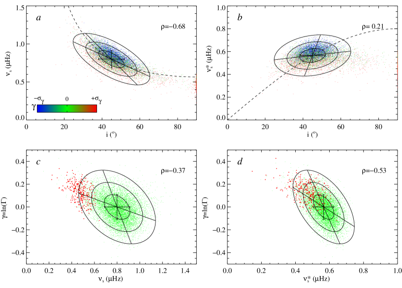
Let us assume as an example for the remaining of this paper a star characterized by $i=45\degr$, $\nu_{s}=0.8\>\mathrm{\mu Hz}$ ($2\Omega_{\sun}$), $\Gamma=1\>\mathrm{\mu Hz}$, and $\beta=1/20$ for $l=1$ modes and $1/10$ for $l=2$. This corresponds to signal-to-noise ratios about five times smaller than those observed for the Sun with VIRGO. We consider here a single $l=1$ multiplet observed for 4 years – that corresponds to Kepler long observation runs – and perform a MC simulation with 10 000 realizations. The theoretical errors and correlations have been deduced from the theoretical Hessian. Figure 3 shows both MC and theoretical results and allow us to verify the consistency of both computations for several pairs of parameters. MC results are shown as clouds of points. From the theoretical Hessian, we have derived the error bars, but also the ellipses of errors and the regression lines to make visible the correlation. We recall that an ellipse of errors is, for a 2D normal distribution, an isoprobability curve given by the equation $Q(\lambda_{i},\lambda_{j})=k^{2}$ where $Q$ is the quadratic

$$Q(\lambda_{i},\lambda_{j})=$$ (23)

$$\frac{1}{1-\rho_{ij}^{2}}\left[\frac{(\lambda_{i}-\mu_{i})^{2}}{\sigma_{i}^{2}}-\frac{2\rho_{ij}(\lambda_{i}-\mu_{i})(\lambda_{j}-\mu_{j})}{\sigma_{i}\sigma_{j}}+\frac{(\lambda_{j}-\mu_{j})^{2}}{\sigma_{j}^{2}}\right]$$

where $\mu_{i}$, $\sigma_{i}$ are the mean values and the standard deviations and $\rho_{ij}$ the correlation coefficient (see §2.2). The number $k$ is a real constant – generally integer – and defines the confidence level: the probability to get a point inside the ellipse is $1-\exp(-\frac{1}{2}k^{2})$.

As for the Sun, the pair of parameters $(A,\Gamma)$ are strongly correlated such $\tilde{A}\tilde{\Gamma}\approx{}$const (not plotted). We have found a correlation coefficient $\rho_{a\gamma}=-0.91$ for our example. This coefficient is almost insensitive to the values of the inclination and the splitting. By exploring different values of $i$ and $\nu_{s}$, we always find a correlation with an absolute value larger than 0.8. This is, of course, independent of choosing either $\nu_{s}$ or $\nu_{s}^{*}$ as a free parameter.

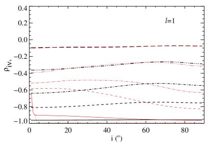
The second strong correlation we observe is between $i$ and $\nu_{s}$ (Fig. 3a). We recover the result of Ballot et al. (2006): for low rotation rate, $(i,\nu_{s})$ are correlated such that $\tilde{\nu}_{s}\sin\tilde{i}\approx{}$const. In our example, the correlation coefficient $\rho_{i\nu_{s}}=-0.68$, and $|\rho_{i\nu_{s}}|$ is even greater than 0.9 for $\Omega=\Omega_{\odot}$. By using $\nu_{s}^{*}$ instead of $\nu_{s}$ (Fig. 3b), the correlation decreases: $\rho_{i\nu_{s}^{*}}=0.21$ for our example, and we have obtained $\rho_{i\nu_{s}^{*}}\approx-0.1$ for $\Omega=\Omega_{\odot}$. It is important to recall that it is true at low rotation rate only; when $x_{s}\gg 1$, the situation is opposite, $i$ is more correlated with $\nu_{s}^{*}$ than with $\nu_{s}$. Figure 4 illustrates, for a $l=1$ mode, the change of $\rho_{i\nu_{s}}$ from -1 to 0 as $\nu_{s}$ increases. We get similar results for $l=2$. The correlation coefficients are deduced from both the full theoretical Hessian and the simplified one proposed in §3.2. We note the limitation of the latter calculation for intermediate values of $\nu_{s}$: for these configuration, that gives the good order of magnitude for $\rho_{i\nu_{s}}$, but an incorrect dependency on $i$.

Figure 4: Correlation coefficient between $i$ and $\nu_{s}$ for an $l=1$ mode as a function of $i$, for different values of $x_{s}$ (see caption of Fig. 1). Black lines show errors obtained with the simplified Hessian, thin red lines are obtained by inverting the full Hessian.

Figures 3c and 3d illustrate the correlation of $\Gamma$ with $\nu_{s}$ and $\nu_{s}^{*}$. We can also see it by looking at the color gradient, which appears on the upper panel. This correlation is significant and is larger with $\nu_{s}^{*}$ than with $\nu_{s}$. That is understandable: the fitting technique has problems distinguishing between the broadening due to splitting and that due to the natural linewidth. We have verified that the correlation decreases strongly when $x_{s}\gg 1$.

Let us finally notice the dense group of points with $\tilde{i}\approx 90\degr$ obtained with the MC simulation (Figs. 3a and b). The phenomenon is discussed in § 6. These peculiar fits are indicated by red dots on Figs. 3c and 3d and we clearly note that, due to correlations, this set of points is shifted – this indicates a noticeable bias especially on $\nu_{s}$. We notice also these points are organized along the regression line at constant $\nu_{s}$, which indicates that, when $i$ is locked at 90°, $\nu_{s}$ is almost blocked around an underestimated values; that is another consequence of the ($i$,$\nu_{s}$) correlation.

Ballot et al. (2006) suggest using $\nu_{s}^{*}$, instead of $\nu_{s}$, at low rotation rate, to improve some averages and avoid some effects of correlations: for instance to estimate a mean splitting, $\langle\tilde{\nu}_{s}^{*}\rangle/\langle\sin\tilde{i}\rangle$ can be a better estimator than $\langle\tilde{\nu}_{s}\rangle$. We have verified this point with a MC simulation of our example. We have performed 2000 realizations of 10 modes (5 $l=1$ modes and 5 $l=2$ modes). The distribution of $\langle\tilde{\nu}_{s}^{*}\rangle/\langle\sin\tilde{i}\rangle$ compared $\langle\tilde{\nu}_{s}\rangle$ exhibits a smaller dispersion (0.10 against 0.15$\>\mathrm{\mu Hz}$ in our case) with a reduced tail at high $\nu_{s}$.

One must also take into account the existing correlations when one computes derived variables such as the total power of a mode $P$. We denote $p=\ln P$. A naive estimation of $\sigma_{p}^{2}$ is $\sigma_{a}^{2}+\sigma_{\gamma}^{2}\approx 0.47^{2}$ (for our example with $T={}$6 months). However due to the correlation, we have to consider the covariance to recover a correct error: $\sigma_{p}^{2}=\sigma_{a}^{2}+\sigma_{\gamma}^{2}+2\sigma_{a\gamma}\approx 0.15^{2}$ (this value is in agreement with those found with a MC simulation, see §5 Fig. 5). This point seems obvious but is frequently forgotten.

Lastly, when it is possible to determine the angle $i$ with other techniques, one can fix it and thus one stands in a position similar to the helioseismology, which is more confortable. However, we have to keep in mind that, due to the complex correlations between all of the parameters, an angle $i$ assigned to a wrong value introduces biases in the determination of other parameters and so introduces systematics which should be estimated on a case by case basis.

5 Biases for $\@vec{\lambda}$ and $\@vec{\sigma}$

$T=6$ months                          $T=4$ years

Figure 5: Distribution of real errors, $\tilde{\lambda}_{j}-\lambda_{j}$, normalized by the estimated errors $\tilde{\sigma}_{j}$ for different parameters (from top to bottom: linewidth, central frequency, splitting, projected splitting, angle and mode power), for two different durations: $T=6$ months (left) and 4 years (right). On each plot, the filled histogram is the distribution when only realizations with $\tilde{i}>89\degr$ are taken into account, dashed line is the standard normal distribution, and the mean value $\langle\tilde{\sigma}_{j}\rangle$ is the error deduced from the theoretical Hessian, quoted in $\mathrm{\mu Hz}$ for $\nu_{0}$, $\nu_{s}$ and $\nu_{s}^{*}$, and in degrees for $i$.

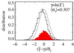
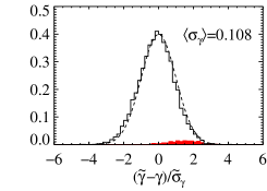
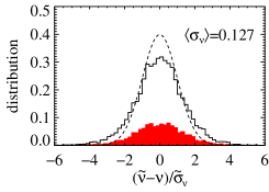
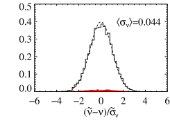
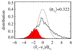
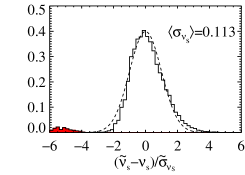
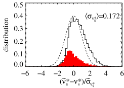
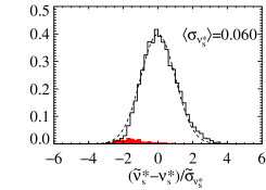
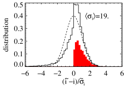
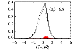
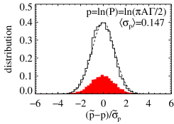
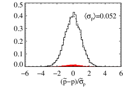
We know that asymptotically, for long observation times, our estimators of parameters $\tilde{\lambda}_{j}$ and their associated errors $\tilde{\sigma}_{j}$ are non-biased (e.g. Appourchaux et al. 1998). However, because observation durations are finite, biases can appear both on $\tilde{\lambda}_{j}$ and $\tilde{\sigma}_{j}$. To study this point, we have used the results of the MC simulation described in the previous section. Asymptotically, for $T\rightarrow\infty$, due to the Central Limit Theorem (CLT), fitted parameters follow normal laws; thus $(\tilde{\lambda}_{j}-\lambda_{j})/\tilde{\sigma}_{j}$ asymptotically follows a standard normal law. Figure 5 shows, for our simulated case, the distribution of the ratio between real errors $\tilde{\lambda}_{j}-\lambda_{j}$ and estimated error bars $\tilde{\sigma}_{j}$ for different parameters and for two different observation durations: 6 months (close to CoRoT long runs) and 4 years (Kepler long runs). These plots allow us to see potential biases on parameter determinations or over/underestimations of errors, by comparing the position and the shape of the distribution relative to the standard normal law.

First, the logarithmic linewidth $\gamma$ is slightly biased after 6 months of observations: fitting tends to underestimate its value. However, the distribution spread is close to the expected one, that indicates correct estimations of errors $\tilde{\sigma}_{\gamma}$. The distribution of logarithmic heights $a$ (not plotted) is very similar to those of $\gamma$, and in particular we find a similar small bias for short times, but in the opposite sense. As a consequence of these opposite biases, the sum of both, i.e. the mode power $p$, is almost non-biased, even for 6-month observations and its distribution is symmetric and almost normal. If we turn now to the central frequency, $\nu_{0}$, we notice no bias for the fitted values $\tilde{\nu}_{0}$, but for 6-month observations, the errors are generally underestimated, as shown by the extended wings of the distribution.

Six months are generally too short to verify the CLT, especially for splitting – projected or not – and angle. The distribution of $\nu_{s}$ is non-gaussian and is moreover highly spread, that indicates $\tilde{\sigma}_{\nu_{s}}$ are significantly underestimated. The distributions of $i$ and $\nu_{s}^{*}$ are less spread than the previous one, but exhibit clear asymmetries, due to biases for both estimated parameters and errors.

After 4 years, all of the distributions are close to normal. Nevertheless, the angle distribution is still asymmetrical and exhibits a slight bias. The distributions of splitting and projected splitting also show a very small asymmetry but become very close to the standard gaussian, that is a noticeable change mostly for $\nu_{s}$.

Let us focus now on the realizations for which fits have been locked at 90°. First, we note that the number of such cases is reduced for $T=4$ years compared to 6 months. Due to correlations, when the fitting converges to $\tilde{i}={}$90°, all of the parameters are expected to be biased; there are few exceptions: the central frequency, because it is not correlated with the other parameters (§3.1), and the mode power, a derived parameter which appears to be almost non-correlated with the angle. Another manner to understand this fact is that, since $i$ only acts on the shape of the multiplet, it does not modify its integral (i.e. the power $P$) or its center of gravity (i.e. $\nu_{0}$). All other parameters are affected, and the bias becomes significantly large for $\nu_{s}$ (greater than $5\tilde{\sigma}$) when $T={}$4 years, which is visible as a bump on the left of the plot. It has already been mentioned in §4 and is visible on Fig. 3c as a set of crosses shifted to the left toward low splitting by about $3\sigma$. These two results seem in contradiction at first sight, but $\sigma$ has a different meaning in Fig. 3c and Fig. 5. From Fig. 3c we learn that, when locking occurs, the mean bias for $\nu_{s}$ is 3 times the mean standard deviation since red dots cluster around the outer ellipse of errors corresponding to the 3$\sigma$ level, whereas Fig. 5 shows that, in such situations, the mean bias for $\nu_{s}$ is 5 times the error bar estimated for the given case. This indicates that, when locking occurs, the error bars for $\nu_{s}$ also are underestimated.

6 Fit locking at $i=90\degr$

Previously, we have seen that a non-negligible proportion of fittings converge toward a solution with $\tilde{i}=90\degr$. This phenomenon has been first observed by Gizon & Solanki (2003). We summarize in Table 1 the fraction of such fits for different situations. Once again, we have considered here our sample star, for several observation durations from 3 months to 4 years. We have fitted single $l=1$ modes, pairs of modes $l=0$ and 2, and also sequences of three modes $l=0$, 2 and 1. $l=1$ modes have been fitted using ($i,\nu_{s}$) or ($i,\nu_{s}^{*}$) as free parameters, and, in one case, all of the other parameters have been fixed to their exact values.

Table 1: Fraction of fitting locked at $i=90\degr$ for different observation times and different sequences of fitted modes

$T$	3m	6m	1y	2y	4y
$l=$1 ($i,\nu_{s}$)	29%	26%	18%	10%	3%
$l=$1 ($i,\nu_{s}^{*}$)		24%			3%
$l=$1 ($i,\nu_{s}$)${\dagger}$		22%
$l=$0&2 ($i,\nu_{s}$)		18%			0.2%
$l=$0,2&1 ($i,\nu_{s}$)		8%			0.2%
${\dagger}$($B,A,\Gamma,\nu_{0}$ fixed)

We can draw several conclusions. As we expect, the fraction decreases when $T$ increases; thus, for Kepler-like observations (4 years), there is almost no problem. Second, the results are almost the same by fitting either ($i,\nu_{s}$) or ($i,\nu_{s}^{*}$), there is no improvement by using $\nu_{s}^{*}$. We notice also that even when we impose the input $A$, $\Gamma$ and $\nu_{0}$, the part of bad fittings is not significatively reduced. This indicates the problem is intrinsic and not just a convergence failure as explained below. Next, since they have more components, $l=2$ modes give slightly better results, though their S/N ratio is lower. However, for $l=2$, another problem appears: in numerous configurations, the fitting hardly distinguishes between a low $\nu_{s}$ with a high $i$, or a lower $i$ with a $\nu_{s}$ two times larger, due to a confusion between $m=\pm 1$ and $\pm 2$ components (See also Gizon & Solanki 2003). Fitting simultaneously $l=1$ and 2 modes allows us to solve this ambiguity. However, although the best results are obtained with sequences of three modes, there are still almost one bad fitting out of ten, for 6-month observations (CoRoT-like observations) – that is not negligible.

Figure 6: Maps of likelihood $\ell=-\ln{\cal L}$ in the plane ($i,\nu_{s}$) for a $l=1$ mode. Top: map of the mean likelihood. Bottom: an example of realization where the locking phenomeoccurs. Black corresponds to the minimum of $\ell$, white to higher values. Fine white or black dotted lines are contours of constant likelihood. Crosses indicate the input values of $i$ and $\nu_{s}$ in the spectum; dashed line indicates $\nu_{s}^{*}={}$const. Solid lines indicate the minima of $\ell$ along $i$ at fixed $\nu_{s}$, i.e. points where $\partial_{i}\ell=0$ and $\partial^{2}_{i}\ell>0$; dot-dashed lines indicate the minima of $\ell$ at fixed $i$; thick lines mean that this is a global minimum, fine lines a local one. On the bottom plot, the cross with errors bars indicates the result of the fit.

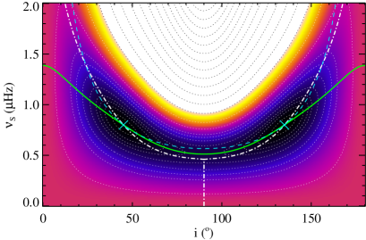
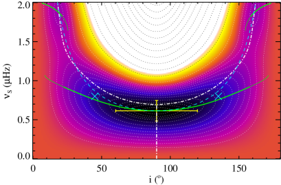
To understand the origin of the fit locking, we have plotted on Fig. 6 (top) the mean likelihood in the plane ($i,\nu_{s}$) for a $l=1$ mode. The plot is symmetric with respect to $\pi/2$ (and $\pi$-periodic). As expected, minima correspond to the values of ($i,\nu_{s}$) used to model the spectrum. Since the likelihood, $\ell$, is even in $i-\pi/2$, a valley along $i=\pi/2$ appears at low splitting, before a fork appears at higher splittings. Obviously the (black) region around the minimum extends up to the limit of 90°, which means that it is quite likely that for a noise realization the minimum of the likelihood will end up close to that limit. It may even end up beyond that limit and in this case because of the periodicity of the inclination there is obviously no inclination which could allow the fit to reach such a minimum. Figure 6 bottom shows an example of such a situation with a global minimum at 90°(and a secondary minimum around 20°, with interestingly the same value of $\nu_{s}^{*}$ since it is also on the dash line). The fit has then been blocked by the hard limit at 90° and has stopped there producing this effect of locking at 90°. A similar effect is described in Chaplin et al. (2008) for a problem of fitting solar-cycle frequency shift or in an ongoing work by the same authors about the zero-locking of $l$=1 splittings for large mode linewidths. All of these problems have a common origin: a parameter is quite sensitive to the realization noise and the minimum of the likelihood function because of the realization noise can take a value which cannot be reached in the parameter range (here 0–90°). In our case to overcome this locking it is sufficient to use a parameter $j=\sin^{2}i$ instead of $i$. If at the minimum, $j$ is larger than 1 it means that the fit using $i$ would have locked at 90°. Of course in this case it is not possible to recover a meaningful inclination. Obviously the locking at 0° is less likely to happen according to Fig. 6 since the black region is confined far from the 0 limit: in other words, the likelihood surface along $i=0\degr$ is a ridge and not a valley as it is along $i=90\degr$. As observations become longer there are more and more points to describe the mode profile and the region is then more confined around the real minimum and further away from the 90° limit, the locking is then less likely to happen unless the underlying inclination is close to the limit itself.

7 Conclusion

As pointed out previously (Gizon & Solanki 2003; Ballot et al. 2006) the extra parameter $i$ introduces difficulties in fitting stellar spectra, compared to the solar case. The main problem originates in the blending of components within a multiplet which strongly correlates the inclination with the rotational splitting, making it difficult to disentangle them. For slow rotators, the uncertainties of $i$ and $\nu_{s}$ are huge (§3.2), because of this. The projected splitting $\nu_{s}^{*}$ appears to be less sensitive to this, thus has more moderate errors. Beyond problems induced by correlations, other issues such as the locking of $i$ at 90° often occur (see §6). The correct derivations of mode heights and linewidths are also dependent on a correct recovering of the inclination.

These issues vanish for stars rotating sufficiently rapidly – or stars with p modes having sufficiently long lifetimes –, if we disregard other issues which appear such as problems in mode identification or blending between different modes. Fixing $i$ before fitting allows us to get around these difficulties. However, due to the numerous correlations between the different parameters (see §4), the value of $i$ must be carefully chosen to avoid systematics.

Nevertheless, even though the value of $i$ modifies the error expected for the central frequency $\nu_{0}$ of a mode (§3.1), it does not introduce any biases as long as the multiplet is symmetric enough (§5). Hence, $\nu_{0}$ should be recovered in any case, as well as certain derived quantities such as the mode power.