Five-Year Wilkinson Microwave Anisotropy Probe (WMAP ) Observations: Beam Maps and Window Functions

Abstract

Cosmology and other scientific results from the WMAP mission require an accurate knowledge of the beam patterns in flight. While the degree of beam knowledge for the WMAP one-year and three-year results was unprecedented for a CMB experiment, we have significantly improved the beam determination as part of the five-year data release. Physical optics fits are done on both the A and the B sides for the first time. The cutoff scale of the fitted distortions on the primary mirror is reduced by a factor of $\sim 2$ from previous analyses. These changes enable an improvement in the hybridization of Jupiter data with beam models, which is optimized with respect to error in the main beam solid angle. An increase in main-beam solid angle of $\sim 1\%$ is found for the V2 and W1–W4 differencing assemblies. Although the five-year results are statistically consistent with previous ones, the errors in the five-year beam transfer functions are reduced by a factor of $\sim 2$ as compared to the three-year analysis. We present radiometry of the planet Jupiter as a test of the beam consistency and as a calibration standard; for an individual differencing assembly, errors in the measured disk temperature are $\sim 0.5\%$.

1 Introduction

The WMAP mission has produced an unprecedented set of precise and accurate cosmological data, resulting in a consensus on the contents of the universe. WMAP has determined the age of the universe, the epochs of the key transitions of the universe, and the geometry of the universe, while providing the most stringent data yet on inflation. At the center of these advances is the angular power spectrum of the CMB, which is the fundamental tool for studying the constituents and density distribution of the early universe.

Characterizing the WMAP beams is crucial to interpretation of the CMB power spectrum. This paper, which describes the WMAP beam analysis based on the five-year data set, is one of seven that together describe the complete five-year WMAP analysis. The results from the suite of papers are summarized and set in context by Hinshaw et al. (2008), which also describes the gain calibration, data processing, and mapmaking.

WMAP observes in multiple microwave frequency bands, namely, K ($\sim 23$ GHz), Ka ($\sim 33$ GHz), Q ($\sim 41$ GHz), V ($\sim 61$ GHz), and W ($\sim 94$ GHz). The sky is observed differentially via two back-to-back offset Gregorian telescopes and associated instrumentation, which are designated side A and side B. The two sides comprise ten independent sets of feed horns and radiometers, called differencing assemblies (DAs): one each in the K and Ka bands, two each in the Q and V bands, and four in W band (Bennett et al., 2003). Each DA is designated by addition of a digit to the name of the frequency band, giving the names K1, Ka1, Q1, Q2, V1, V2, W1, W2, W3, and W4, respectively; thus, for example, Ka is a frequency band, and Ka1 is the corresponding DA.

The terminology applied to beams can be subtle, and it reflects, to some extent, the details of the particular analysis that is done. Here, we give a brief overview. For a fuller exposition of beam-related concepts and notation, the reader is referred to Page et al. (2003a) for the main beams and Barnes et al. (2003) for the far sidelobes. The WMAP optics are described and analyzed in Page et al. (2003b).

We can directly make a measured beam for any DA, either separately for the A and B sides, or by averaging the two sides. Similarly, we can make beams for either of the two radiometers in a DA, which measure orthogonal polarizations, or combine the two. In a strict sense, the word beam means point-source response in spherical coordinates, covering the full $4\pi$ steradians. We divide the full beam into two parts, which are measured differently and treated differently in the analysis: the main beam and the far sidelobes. The main beam has a radius of $3\fdg 5-7\arcdeg$ depending on the DA. The measured main beam includes observations of Jupiter, while the measured far sidelobes include in-flight observations of the Moon, as well as pre-flight laboratory data.

The A- and B-side main beams can be predicted using physical models of the WMAP optics. Indeed, we go further and adjust the model parameters in an iterative $\chi^{2}$ fit to arrive at model main beams, or more simply, beam models. The instrument parameters of interest are small surface distortions of the mirrors, especially the two primaries. Mirror distortions are modeled as low-amplitude Fourier or Bessel modes added to the nominal mirror shapes. At intermediate angular scales within the main beams, the models are actually more reliable than observations, so that we combine models and observations to produce hybrid beams.

An additional variation in terminology is produced by our attempt to reconcile the farthest outskirts of the model main beams with the far-sidelobe observations of the Moon. In this part of the analysis, the parameter set of the best-fit model is augmented with extrapolated small-scale distortions of the primary mirror to produce augmented beam models.

Scan strategy combines with the inherent geometry of each beam to produce maps with effective beams that are nearly azimuthally symmetric, when averaged over each year of observations. The beam analysis results in a symmetrized beam profile, which is equivalent to a symmetrized point-spread function in optical astronomy. The transform of the beam profile in harmonic space is termed a beam transfer function, $b_{\ell}$. A raw CMB power spectrum is divided by $w_{\ell}=b_{\ell}^{2}$ to invert the filtering done by finite-width beams, and the resulting beam-corrected power spectra are used for fitting cosmological parameters; $w_{\ell}$ is called the window function.

Beam measurements consist of repeated scans over the planet Jupiter by each DA, which occur as part of the standard WMAP full-sky observing strategy, with no need for special observations (Bennett et al., 2003). Jupiter is effectively a point source that allows high-resolution sampling of each beam. Because the sky is covered completely in six months, every observing year includes two Jupiter seasons, each lasting $\sim 50$ days. The data taken when Jupiter is near the axis of each of the twenty main beams are extracted from the time-ordered data (TOD) archive and analyzed separately from the sky map processing. Thus, the Jupiter data are reduced in the same manner as the CMB data in terms of baseline removal and gain calibration (Hinshaw et al., 2008). Each brightness sample is labeled with the instantaneous position of Jupiter’s image in the A-side or B-side focal plane. These data may be either utilized in time-ordered form or accumulated into twenty two-dimensional beam maps.

The first-year beam analysis was described in Page et al. (2003a). For each DA, the beams for the largely symmetric A and B optics were measured independently. Azimuthally symmetrized beam profiles were fitted to the time-ordered data (TOD) of Jupiter using Hermite functions as the basis. The A- and B-side beams were averaged to give one beam per DA. Mean asymmetry corrections were produced by a time integration of the beam orientation.

The first-year beam analysis also included the fitting of the detailed shapes of the primary and secondary mirrors, motivated in part by the fact that the cold, laboratory-measured rms of the primary mirror surface distortions did not meet the pre-flight specification (Page et al., 2003b, §2.6). Inputs to a physical optics modeling program, DADRA (Rahmat-Samii et al., 1995), were varied iteratively to match Jupiter data. This program requires four types of inputs: (1) as-built coordinates and Euler angles of the primary and secondary mirrors and the feed horns, on both the A and the B sides; (2) as-designed feed horn outputs expressed as a spherical-wave approximation; (3) as-built primary and secondary mirror shapes; (4) perturbation coefficients for small distortions of the mirror shapes, which were fitted as free parameters. In the first-year analysis, the fit was done only on the A side and was used mainly to check the integral of the peak-normalized beam, called beam solid angle (Page et al., 2003a).

The three-year beam analysis was described in Jarosik et al. (2007). With the increase in the number of Jupiter seasons, the physical optics fits became well enough constrained to allow the model beams to be extrapolated below the noise level of the data; thus, the models entered directly into the adopted beam profiles. Directly measured beam points based on Jupiter were replaced with predicted values from a beam model if the corresponding model point had a gain below some defined threshold $B_{\mathrm{thresh}}$. This merger, or hybridization, was done before Hermite function fitting. Again, the physical optics modeling was applied only to the A side, and the result was transformed to be applicable to the B side. Also, residual departures from azimuthal symmetry in the scan-averaged beams were computed for each DA and found to be subdominant, except in Q band at $\ell\gtrsim 500$ (Hinshaw et al., 2007). Beam errors were computed to encompass the overall uncertainty in the data, the modeling, and the transformation from A side to B side.

The five-year beam analysis is the main subject of this paper. An additional four seasons of Jupiter observations have increased the signal-to-noise ratio ($S/N$) of the beam data, allowing the boundaries of the main beams to be expanded to lower gain levels. The scope of the physical optics fitting has been extended in two main ways. First, separate, complete fits are now done on both the A- and the B-side optics. Second, the cutoff scale of the fitted distortions on the primary mirror is reduced by a factor of $\sim 2$, in effect widening the beam area that is treated by the models. The hybridization step has been changed in that it is now optimized statistically, by minimizing the error in the beam solid angle. The hybrid beam profiles are transformed directly to $b_{\ell}$, with no intervening functional fit. The improved $S/N$ and modeling result in a $\sim 1\%$ increase in the solid angle of the adopted main beam for several DAs, occuring mainly inside the old beam radius. However, the new beam transfer functions are consistent with those from the two earlier analyses.

The five-year results include a revision to the WMAP full-sky sidelobe sensitivity patterns. Augmented beam models, which are matched to early-mission observations of the Moon, are substituted for a part of the sidelobe measurements taken under ambient ground-based temperature and humidity. In addition, the in-flight Moon observations used directly in the sidelobe patterns are recalibrated for bands Ka–W. The resulting patterns are used in WMAP sky map generation to correct for sidelobe pickup.

An important test of the consistency of beam processing is radiometry of the planet Jupiter. These measurements, which should also be useful in calibrating other microwave observations, are presented here, together with radiometry of Mars and Saturn.

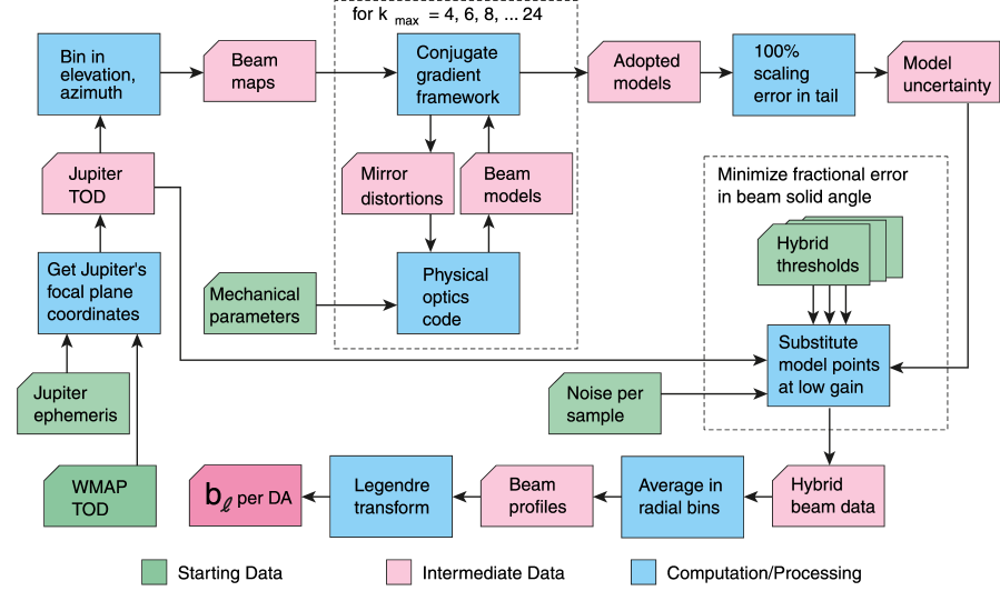
A flowchart of the main beam processing, from TOD through window functions, is shown in Figure 1. This processing is described in detail in §2, which describes the fitting of model beams, and in §3, which describes the computation of beam transfer functions from Jupiter observations and models. Radiometry of selected planets is given in §4. The conclusions of this study are summarized in §5.

2 Physical Optics Models

2.1 Beam Data

The fundamental beam data are Jupiter measurements extracted from the mission’s TOD archive. These measurements are differential like all WMAP data, but the presence of Jupiter in only one of the two beams of a given DA means that they are effectively single-dish, after subtraction of a differential sky background. Five-year WMAP full-sky maps, which omit Jupiter, are used to estimate this background. Also, measurements affected by a bright source other than Jupiter in either set of optics are omitted. The apparent measured Jupiter temperatures are scaled to a standardized distance of 5.2 AU and are binned by the position of Jupiter in a coordinate system attached to the spacecraft. Planetary coordinates are obtained from the Jet Propulsion Laboratory ephemeris DE200(Standish, 1990).

2.2 DADRA Modeling

2.2.1 Software Structure

The physical optics modeling is the most computationally intensive aspect of the WMAP beam analysis. Individual fitting runs can take days or weeks, even with the availability of numerous processors. The procedure is automated as much as possible to minimize user intervention and false starts.

Several pieces of software are used in concert. Computation of a beam model from a specification of the mirrors and of a single feed is done by a Fortran program called DADRA (Rahmat-Samii et al., 1995). The overall framework of the fitting algorithm is embodied in an Interactive Data Language (IDL) code, which performs a conjugate-gradient $\chi^{2}$ minimization driven by the residuals between beam models and the Jupiter data. Requests for beam computations are made by the IDL program, and they are passed to DADRA by intermediary shell scripts running continuously in the background. This architecture enables the computation to be spread over multiple processors, with each processor running an instance of DADRA.

The minimization software is in most respects the same as that used in the first two WMAP beam analyses (Page et al., 2003a; Jarosik et al., 2007). In the one- and three-year analyses, ten processors of one computer were used concurrently to compute the beams for a given mirror distortion. However, for the five-year fits, upgrades to the IDL and shell code enable the use of multiple computers. Typically, the fit uses four to six clustered Silicon Graphics Origin 300 machines, each with 32 processors and 32 gigabytes of memory in a non-uniform memory access (NUMA) architecture. With these resources, 12 to 18 sets of ten beam models each can be computed simultaneously.

2.2.2 Parameters of Fit

The coordinates and Euler angles of the WMAP optical components are furnished to DADRA as constants, as are the measured mirror shapes and the beam patterns of the feed horns. These constants are results of the pre-flight structural thermal optical (STOP) performance analysis (Page et al., 2003b). The fit is done by varying a set of mirror distortion parameters, which are defined as small-amplitude Fourier or Bessel modes added to the input shape. The emphasis in the fitting is on the primary mirror, because in pre-flight laboratory measurements, the shape of the secondary was less susceptible to temperature changes. Also, the illumination pattern occupies a much larger proportion of the primary mirror than of the secondary (Page et al., 2003b, Figure 2). For these reasons, the perturbation space chosen to characterize the primary mirror encompasses more modes than that for the secondary. Moreover, Fourier modes in $x$ and $y$ are a natural choice because the morphology of the distortions is dominated by a rectangular frame that is part of the backing structure. On the other hand, the mount of the secondary is cylindrically symmetric with a more extensive backing structure, consistent with fitting to a restricted set of Bessel modes.

The primary distortions have the form

$$\delta Z = \sum C(k_{x},k_{y})\cos\left({2\pi k_{x}x\over L}+{2\pi k_{y}y\over L}\right)\$$

$$+\sum S(k_{x},k_{y})\sin\left({2\pi k_{x}x\over L}+{2\pi k_{y}y\over L}\right)\$$

$$+\sum_{\mathrm{special}}A_{\mathrm{sp}}F_{\mathrm{sp}}(x,y).$$

The distortion modes are characterized by the spatial frequency indexes $k_{x}$ and $k_{y}$, where $k=1$ corresponds to $L=280$ cm, which is twice the width of the mirror. The reason for setting $L=280$ cm rather than $140$ cm is to remove the requirement that the solution be periodic on the circumscribed square; in particular, an approximate tilt of the $140$ cm mirror is expressed naturally as half a sine wave with a $280$ cm period. Some of the Fourier modes specified in this way are redundant, so the set that is used in the fit is culled to contain only even values of $k_{x}$ and $k_{y}$, with $k_{x}>0$. A few additional modes with $k_{x}$ and $k_{y}$ of $\pm 1$ are the ones that represent tilt. Special distortion modes, $F_{\mathrm{sp}}(x,y)$, are also allowed, with amplitudes $A_{\mathrm{sp}}$. One special mode is a scalar offset of the whole mirror surface. A second special mode is simply a map of the mirror surface as measured pre-flight; in practice, this mode plays no significant role in the fit. The phase and strength of the modes are specified by the sine and cosine amplitudes, $S(k_{x},k_{y})$ and $C(k_{x},k_{y})$, and the amplitudes of the special modes, $A_{\mathrm{sp}}$. Below, we make use of the power per mode, $P(f)=C(k_{x},k_{y})^{2}+S(k_{x},k_{y})^{2}$, where $f$ is the spatial frequency in $\textrm{cm}^{-1}$ and $f^{2}=(k_{x}/280)^{2}+(k_{y}/280)^{2}$.

The three-year fit, carried out for the A side only, reached a maximum spatial frequency index of $k_{\mathrm{max}}=12$, corresponding to a distortion wavelength of $280/12\sim 23$ cm. By contrast, the five-year fit reaches $k_{\mathrm{max}}=24$, or $\sim 12$ cm, for both the A and the B sides. The number of Fourier modes goes as $k_{\mathrm{max}}^{2}$, so the five-year fits include $\sim 400$ modes on each primary as compared to $\sim 100$ modes in previous analyses. This extension in $k$ space means that the primary mirror distortions are fitted nearly to the surface correlation length measured in the laboratory under cold conditions, i.e., 9.3 cm on the A side and 11.4 cm on the B side (Page et al., 2003b).

The secondary mirror distortions are described by Bessel functions:

$$\delta Z=\sum_{n,k}J_{n}(\nu_{n,k}\rho/L)[C_{n,k}\cos(n\phi)+S_{n,k}\sin(n\phi)]\ ,$$ (1)

where $\rho$ and $\phi$ are cylindrical coordinates and $L$ is the radius of the mirror. The $k$th alternating zero of $J_{n},J^{\prime}_{n}$ is denoted $\nu_{n,k}$; zeroes of $J_{n}$ have $k$ odd, and zeroes of $J^{\prime}_{n}$ have $k$ even. Inclusion of the zeroes of $J^{\prime}_{n}$ removes any constraint on the edge of the mirror. The fitted parameters are $C_{n,k}$ for $n\geq 0$ and $S_{n,k}$ for $n\geq 1$. Two different pairs of $(n_{\mathrm{max}},k_{\mathrm{max}})$ are used: $(1,3)$, resulting in nine parameters, or $(2,6)$, resulting in 30 parameters.

2.2.3 Fitting Method

The optimization is done by a modified conjugate gradient method, a deterministic descent into a $\chi^{2}$ valley. Avoidance of local $\chi^{2}$ minima is attempted by exploiting the Fourier description of the primary mirror distortions. The largest scale distortions are fitted first, and each result is used as a starting point for the next fit, in which finer scale modes are included. At each stage, distortions at the large scales that have already been fitted are not held constant, but rather, they are refitted together with the small-scale distortions that are newly included.

As defined above, the primary mirror modes do not compose an orthogonal basis. However, orthogonality is desirable in order to make the fit as efficient as possible. Consequently, the primary mirror modes are not fitted directly, but first are orthogonalized with respect to the area inside the circular boundary of the mirror, using a modified Gram-Schmidt method. When the $k_{\mathrm{max}}$ of the included Fourier modes is increased, a new orthogonalization is performed that generates a completely new set of linear combinations of the Fourier and special modes. The conjugate gradient algorithm therefore navigates in a space consisting of two groups of parameters: (1) the amplitudes of the orthogonalized primary mirror modes, and (2) the amplitudes of the Bessel modes on the secondary.

Each time $\chi^{2}$ is calculated, two types of adjustment are made to the model beams. First, the pointing in the coordinate frame attached to the spacecraft is matched to that implied by the Jupiter observations. Second, the peak sensitivity of the model is scaled to match the peak observed Jupiter temperature. The pointing adjustment may be done for the ten beams as a group, without altering their mutual displacements, or it may be done for each beam separately. However, the peak scaling is always done separately for each beam.

These adjustments are not parameters of the fit, because corresponding dimensions of $\chi^{2}$ space do not exist. Rather, their purpose is to absorb errors in the input coordinates and angles of optical components and prevent them from being projected into the mirror distortions. Ideally, this problem would be avoided by solving a more complicated problem, i.e., by directly fitting the mechanical parameters of the WMAP components. However, a full set of mechanical parameters would include many degeneracies with respect to the beam morphology. By limiting the parameter set to $\sim 100-400$ mirror perturbation modes and ignoring “nuisance” information, we converge on acceptable values of $\chi^{2}$.

For a given fitting run, either the primary or secondary mirror parameters can be held constant at the starting values. The DA microwave frequencies can also be fitted as parameters, but are held constant in practice, since they are accurately determined.

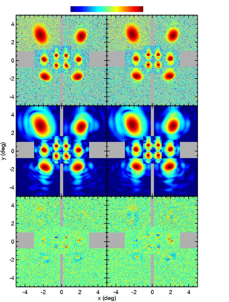
The fits for side A begin with the inherited three-year solution (Jarosik et al., 2007). The final run for each value of $k_{\mathrm{max}}$ is listed in Table 1. An indication of the quality of fit after each step is given by the $\chi^{2}_{\nu}$ column in the table.

The B side of the instrument is characterized by an overall shift of the ten beam pointings in relation to their pre-flight positions, by $\sim 0\fdg 1$. This shift complicates the fitting strategy. The overall fitting history for side B comprises several different sequences of fits. The most important sequence, leading to the adopted beams, is similar to the A-side fitting sequence, in that $k_{\mathrm{max}}$ is increased in stages, with the secondary mirror distortions held constant after being fitted early in the sequence (Table 2). In other sequences, a different form of the secondary was tried, the floating shift in elevation and azimuth was disabled, or the secondary alone was fitted from various initial conditions. None of these variations improved $\chi^{2}$ for the resulting beams, as compared to the adopted fitting sequence.

The fitted beams and residuals for sides A and B are shown in Figure 2, which can be compared to Figure 9 of Jarosik et al. (2007).

2.2.4 Instrument Parameter Results

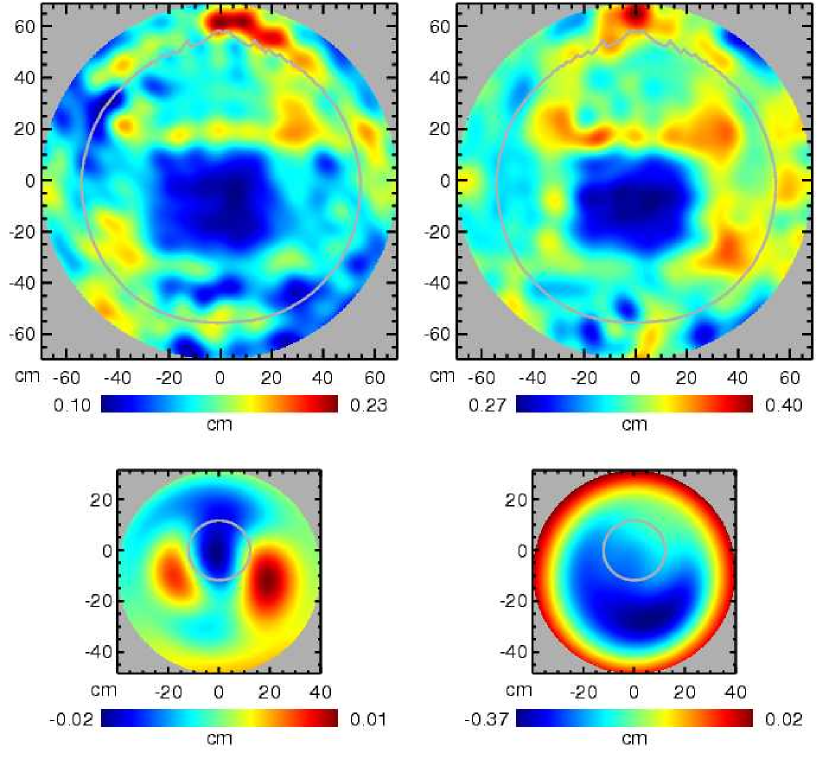
False-color renditions of the final A and B side mirror surface fits are shown in Figure 3. Two natural length scales for the surface of the primary mirrors are $0.5$ cm for a hexagonal mesh that composes one layer of each mirror, and $30$ $\mu$m for the correlation length of the reflector surface roughening, which was done to diffuse visible solar radiation (Page et al., 2003b). Both of these length scales are too small to be probed either by the direct fitting of the main beam or by the sidelobe observations of the Moon. The main feature of each fitted primary mirror figure is the backing structure, dominated by members that form a rectangular frame near the center of the mirror. In the center part of this rectangle, the primary mirror appears to be depressed by $\sim 0.5-1$ mm. Also seen are hints of the stiffening lugs near the edge of each backing structure. The rms distortions of each primary mirror model are $\sigma_{z}=0.023$ cm and $0.022$ cm for the A and B sides, respectively. Pre-flight cold-measured values on the real mirrors, as extrapolated to the flight temperature of 70 K, were $\sigma_{z}=0.023$ cm and $0.024$ cm, respectively (Page et al., 2003b).

For the A side, the measured centroids of Jupiter beam data are displaced by $\sim 0\fdg 03\pm 0\fdg 02$ from the nominal pre-flight beam positions on the sky, where the error term is the $1\sigma$ scatter among beams. However, for the B side, the corresponding displacement is $0\fdg 13\pm 0\fdg 03$. The $\chi^{2}$ computation in the beam-fitting algorithm includes a floating elevation-azimuth adjustment that is intended to soak up such discrepancies without converting them into parameters of the fit. For the final adopted beam models, the floating displacement amounts to $0\fdg 09$ in combined elevation and azimuth for side A, and $0\fdg 21$ for side B. The difference between these two values agrees with the raw pointing difference between the beams on each of the two sides.

We emphasize that these displacements are unrelated to the estimated pointing errors of $<10\arcsec$ in the WMAP TOD (Jarosik et al., 2007). The A-side and B-side boresight vectors are accurately determined from flight data as part of the TOD processing and are not influenced either by the beam fitting or by pre-flight predictions. The WMAP pointing model is described in Limon et al. (2008).

The mirrors are constrained only where they are substantially illuminated by the feed horns; see Page et al. (2003b), Figure 2. Thus, for example, the secondary mirror for the B side appears as a bull’s-eye partly because the fit is only constrained in the center (Figure 3). In actuality, the fitted shape consists mostly of a tilt of $\sim 0\fdg 25$; however, apparent mirror tilts reflected in the fitted parameters are difficult to interpret because they are coupled to the floating elevation-azimuth offsets.

The polarization characteristics of the main beam models are consistent with previous results. The morphology of the co- and cross-polar components of both the A- and the B-side models is similar to that found for the A side in the three-year analysis. Similarly, cross-polar suppression, as calculated from peak model values, is within $\sim 0-2$ dB of previously reported A-side values, depending on the DA. However, for Q, V, and W bands, the polarization isolation of the orthomode transducer (OMT) dominates the end-to-end cross-polar response, which was measured pre-flight (Jarosik et al., 2007).

2.3 Extrapolation to Small Distortion Scales

The modeling of primary mirror distortions with $k$ as high as 24, which affect the beam at relatively wide angles, raises the possibility of comparing DADRA-computed main beams to the innermost parts of the far sidelobe patterns, which are obtained from observations of the Moon (Barnes et al., 2003).

The beams at angles greater than $5\arcdeg-10\arcdeg$ from each boresight may be affected by unmodeled primary mirror distortions with $24<k\lesssim 250$. However, extending the models to fit these distortions directly is computationally unmanageable, because the required number of Fourier modes is of order $10^{4}$, which is $\sim 100$ times the number of modes in our normal fits. Nevertheless, the observed sidelobe data provide a constraint on the contribution of such modes to the primary mirror surface shapes, and hence to the main beams. To apply this constraint, we need an appropriate choice of sidelobe data together with a method for extending each main beam model to the low gain levels outside the main beam radius.

The choice of sidelobe data is important, because the full-sky sidelobe patterns are dominated by features that are not captured in the beam models. The WMAP sidelobe patterns are depicted in Figure 2 of Barnes et al. (2003). The most vivid features are formed by reflections from the radiator panels, by diffraction around the edges of the primary mirrors, and by reflection from the focal plane assembly. Despite their striking appearance in the referenced figure, these features are at least $40-60$ dB below the peak gain of each main beam; however, they must still be excluded from the comparison.

Only a small region of each sidelobe map, a smooth region in the “shadow” of the primary mirror, is suitable for comparison with the main beams. Although we choose the boundary of this region as conservatively as possible, the choice is subjective and a source of systematic error. Essentially, we draw the boundary according to a combination of sidelobe morphology and angular proximity to the main beam. However, the morphological criterion by nature cannot exclude an extraneous component of sidelobe response that happens to be smooth, such as might arise from a diffuse reflection off the top of the structure that holds the feeds. For this reason, the sidelobe patches chosen for the comparison are regarded as upper limits.

Additionally, these radiometric observations cannot be calibrated as well as the CMB data, primarily because they were taken when the spacecraft was thermally unsettled, during the phasing loops between the Earth and the Moon. The instrumental gain in this part of the mission is estimated to be known to $\lesssim 10\%$. A total of $4.3$ days of Moon data were obtained covering $\sim 1.2\pi$ sr of sidelobe area. The calibration standard for the Moon observations is the COBE DMR model of lunar microwave emission as a function of phase angle (Bennett et al., 1992).

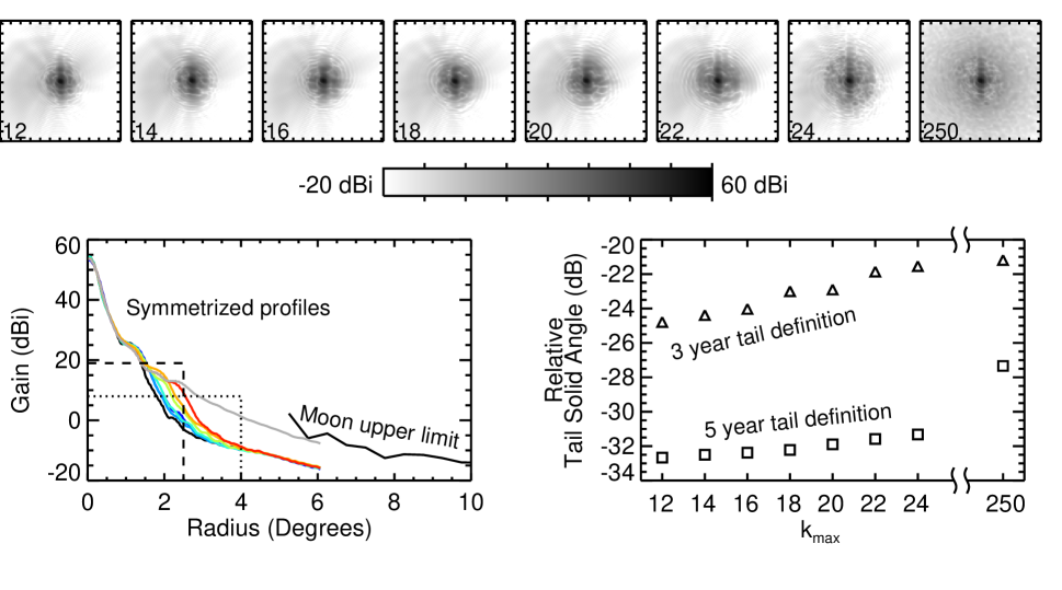
In order to achieve a comparison with the Moon observations, the spatial frequency of the modeled primary mirror distortions is pushed to as high a value as possible. Figure 4 (lower left panel) shows radial profiles of the symmetrized main beam models in comparison to the sidelobe sensitivity pattern for one example beam, V2 on the A side. The sensitivity profile at intermediate angles of $1\fdg 5-2\fdg 5$ is directly related to $k_{\mathrm{max}}$ of the fit, as seen also in the grayscale images of the model beams (top row). A natural hypothesis is that an even greater increase in $k_{\mathrm{max}}$ might give a model that joins smoothly to the Moon data. Unfortunately, the direct fitting algorithm cannot accommodate an indefinite increase in $k_{\mathrm{max}}$, because the number of Fourier modes goes as $k_{\mathrm{max}}^{2}$.

To cope with this difficulty, an approximation is used for Fourier modes with $25\leq k\leq 250$. Power spectra, $P$, of the fitted A-side and B-side primary mirror distortions are shown in Figure 5 as a function of spatial frequency, $f=k/280$ cm^-1. The form of the power spectrum expected from ground-based measurements of the mirrors is also shown, under the assumption of a Gaussian two-point correlation function (Page et al., 2003b). As the spatial frequency increases, $P$ decreases. Our approach is to extrapolate the power spectrum $P(k)$ to smaller scales assuming a power-law form, $P\propto(1/k)^{\alpha}$, with $3\lesssim\alpha\lesssim 6$. Random phases are used to convert the extrapolated spectrum to sine and cosine amplitudes.

A grid of beam models is assembled as a function of two variables: the slope $\alpha$, and the random number seed $s$ that selects the phases used for the extrapolated Fourier modes. Separately for each $s$, a $\chi^{2}$ minimization is used to fit the beam models to the Moon sidelobe data as a function of the slope $\alpha$. The sidelobe maps are in HEALPix format (Gorski et al., 2005) with $\texttt{nside}=512$, and the beam models are resampled onto the HEALPix grid. The value of $\chi^{2}$ is computed from measured and predicted gains, $g$, as $\sum(g_{\mathrm{pred}}-g_{\mathrm{Moon}})^{2}/\sigma_{\mathrm{Moon}}^{2}$, where the sum is over pixels in the region of overlap between the beam model and the Moon data. The fit uses all of the Q, V, and W DAs together. For each side, the fitted values of $\alpha$ from five values of the seed $s$ are averaged to get the adopted slope. Using this slope value, five new beam models are computed with the original phases, and these models are averaged. The result is termed the augmented beam model.

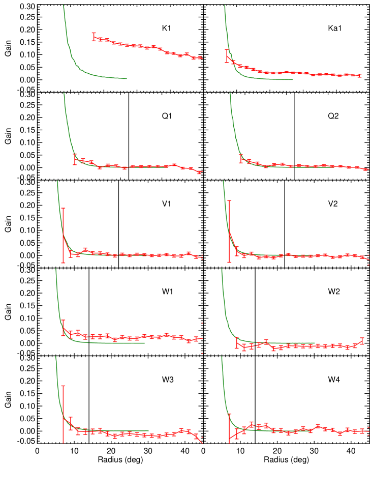
Figure 6 shows radial profiles of the A-side augmented beam models compared to the fitted subset of Moon data. The K1 and Ka1 beams are not used in the fit because of the relatively strong diffuse light that is seen as the bright profile in the top two panels of Figures 6 and 7. This component, which may result from reflection off the focal plane assembly, is seen in Figure 2 of Barnes et al. (2003), where it appears as a haze in the region above the main beam. In addition, the Q, V, and W bands appear subject to systematic errors depending on the individual DA.

For CMB analysis, the main implication of the augmented models is an increase in main beam solid angle as compared to the ordinary fitted models with $k_{\mathrm{max}}=24$. The effect on the “tail” part of the main beam model is illustrated in the bottom right panel of Figure 4. To compute accurately the effect that the augmented models would have on the symmetrized beam profiles used to compute $b_{\ell}$, a hybridization with Jupiter data is required, as described below (§3.1). If augmented rather than ordinary $k_{\mathrm{max}}=24$ beam models are used in the hybridization, the resulting increase in main beam solid angle is just $\sim 0.1-0.3\%$ depending on DA.

There are two arguments for treating this main-beam solid angle increase as an upper limit. One argument is the one already made above, namely, that the Moon data in all bands may include a diffuse reflected component in addition to the extended main beam response, as is apparent for K1 and Ka1, and which our procedure cannot exclude. The other argument invokes the thermal nature of the CMB power spectrum, which requires that the power spectrum be the same in all microwave frequency bands. Section 3.4 below shows that the ordinary models with $k_{\mathrm{max}}=24$ maintain a tighter consistency of the CMB $C_{\ell}$ across Q, V, and W than do the augmented models. Consequently, the adopted 5-year beam transfer functions incorporate only the ordinary models, whereas the augmented models are used to characterize the innermost part of the sidelobe response (§3.2).

3 Beams and Window Functions

3.1 Hybridization

To mitigate sensitivity of the window functions to observational noise, we use a beam hybridization technique similar to that employed in the three-year data analysis (Jarosik et al., 2007). In this method, a hybrid beam is constructed for each DA on each side by combining Jupiter observations with the physical optics models. Jupiter observations are used in the central portions of the beam where $S/N$ is high. Model points are substituted for the data in the outlying regions of low signal, called the tail.

The five-year analysis differs from that of Jarosik et al. (2007) in the method for choosing the hybridization threshold, $B_{\mathrm{thresh}}$, which defines the tail region. In the three-year analysis, the threshold for each DA was chosen to replace noise-dominated parts of the beam with model values, in order to facilitate fitting the beam profile with a smooth function. However, the improvements in the five-year data and modeling open the possibility of extrapolating the main beam to wider angles and subsuming more of the full-sky beam solid angle into the main-beam treatment, rather than the sidelobe pattern. As a result, lower-signal parts of the beam are included in the beam transfer functions, and we require an explicit optimization of $S/N$ in the hybrid beams.

The effect of the beam tail on science occurs through the normalization of the CMB power spectrum, $C_{\ell}$. An increase in main beam solid angle raises the beam-corrected $C_{\ell}$ by a constant factor for $\ell\gtrsim 100$. Hence, the error in the solid angle is a convenient indicator of the error induced in the high-$\ell$ part of the CMB power spectrum via the hybridization. The solid angle error is therefore a natural figure of merit for optimizing $B_{\mathrm{thresh}}$.

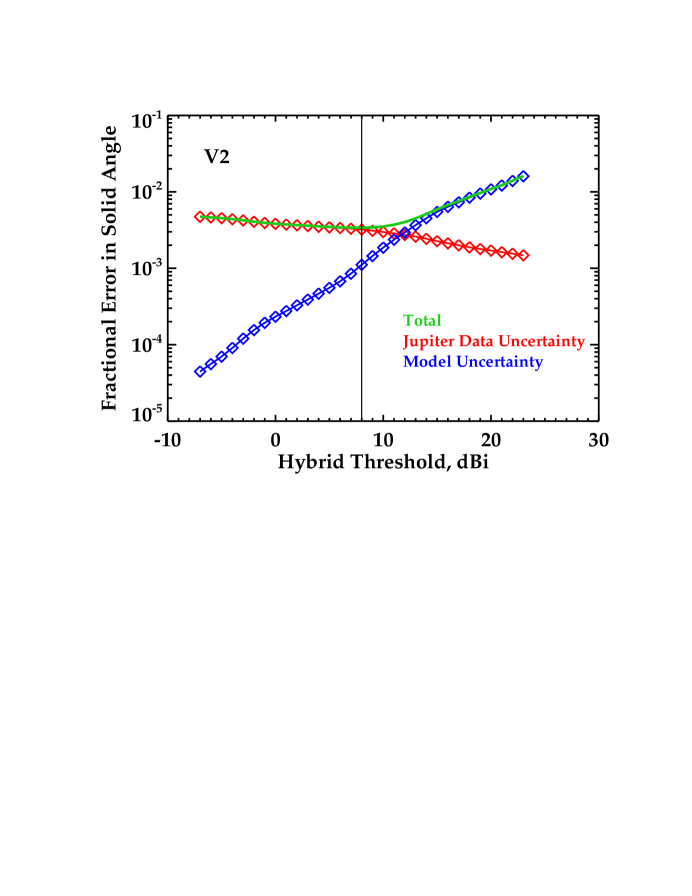
A grid of simulations is run that evaluates solid angle error in the hybrid beam as a function of threshold level. Let the true solid angle of a given beam be $\Omega$, and the solid angle of the hybrid beam be $\Omega_{h}(t)$, where for conciseness we use $t$ to stand for $B_{\mathrm{thresh}}$. Then, $\Omega_{h}(t)=\Omega_{d}(t)+\Omega_{m}(t)$, where $\Omega_{d}$ is the portion taken from data, and $\Omega_{m}$ is the portion taken from the model. Another way of decomposing $\Omega_{h}$ is into a true solid angle and error terms, i.e., $\Omega_{h}=\Omega+e_{d}(t)+e_{m}(t)$, where $e_{d}(t)$ is the error in the data portion for threshold $t$, and $e_{m}(t)$ is the error in the model portion. The model error can be parametrized as a fraction of the model solid angle, such that $e_{m}(t)=a\Omega_{m}(t)$. If $e_{m}$ is uncorrelated with $e_{d}$, then the fractional variance in $\Omega_{h}$ is

$$\mathrm{Var}\{\Omega_{h}(t)/\Omega\}=\mathrm{Var}\{e_{d}(t)/\Omega\}+\mathrm{Var}\{a\}(\Omega_{m}(t)/\Omega)^{2},$$ (2)

and the hybridization threshold is chosen to be the value minimizing this variance.

Essentially, the variable $a$ in the above discussion is a scaling error that is common to all of the model points incorporated in the hybrid beam. A conservative method of estimating systematic error is to assume that it is of the same order as the quantity estimated. In the above formulation, we represent this estimate by setting $a=1$.

Figure 7 shows the fractional error in the hybrid beam solid angle for the V2 beam on the A side, as a function of $B_{\mathrm{thresh}}$. To avoid a selection bias, $B_{\mathrm{thresh}}$ is referred to the model rather than the data. The errors contributed by the data portion and the model portion are shown along with the total error, which is computed using Eq. 2 with $a=1$. For the data, the solid-angle error is obtained as a function of $B_{\mathrm{thresh}}$ from 100 Monte Carlo simulations in which model input beams are combined with white noise appropriate to the Jupiter data for each DA. The contribution of the data portion increases with lowered threshold as more of the noisy data are included in forming the hybrid beam. Conversely, the contribution of the tail portion decreases with lowered threshold as less of the model is included. The adopted $B_{\mathrm{thresh}}$ values for the five-year analysis are obtained from the locations of minimum total error in similar plots made for all the A- and B-side beams. These values are shown in Table 3 together with the three-year equivalents. The five-year thresholds are lower than the three-year thresholds by some $5-10$ dB, depending on DA. Thus, we use significantly more of the data than we have in the past.

3.2 Sidelobes

For the five-year analysis, changes have been made in the sidelobe sensitivity patterns that are distributed as part of the data release. These patterns are in linear units of gain relative to isotropic, and they are assembled from several types of data, including the Moon observations described above. In previous analyses, the conversion of observed Moon brightness to gain assumed a temperature of 175K for the Moon. However, in K band the resulting gains were divided by 1.3 to match adjacent pieces of the sidelobe pattern that were derived from other data (Barnes et al., 2003).

For the five-year analysis, the calibration has been improved by integrating the COBE DMR model of lunar microwave emission (Bennett et al., 1992) over the spacecraft and Moon ephemerides. This procedure lowers the gain values in the Moon-derived parts of the sidelobe pattern by factors of 1.35, 1.39, 1.45, and 1.51 for the Ka, Q, V, and W bands, respectively, while confirming the earlier adopted calibration of K band.

Additionally, some ground-based beam measurements, used within $\sim 10\arcdeg$ of each boresight, have been replaced with the augmented main beam models described above (§2.3). The ground-based data were taken under ambient conditions in the Goddard Electromagnetic Anechoic Chamber (GEMAC), where the primary mirror distortions are different from those under flight conditions. This replacement affects at most $\sim 0.5\%$ of the sky for any given DA.

In the sidelobe reponse patterns, the area inside the main beams is set to zero. This area is expanded for the five-year analysis (§3.3).

The differential signals tabulated in the WMAP TOD archive are corrected for sidelobe contamination. The overall effect can be summarized in one number for each DA, called the sidelobe recalibration factor, which is the factor by which the correction changes the instrumental gain (since the dipole is detected in the sidelobes along with other sources). A sidelobe recalibration factor of unity means that the sidelobe response is zero. In the three-year analysis, these factors differed from unity by $0.3\%-1.5\%$ (Jarosik et al., 2007), and for the five-year analysis, they differ from unity by $0.05\%-1.4\%$ (Hinshaw et al., 2008). The decrease in the sidelobe correction is caused by the increased main beam area together with the lower calibration of the Moon data.

3.3 Symmetrized Beam Profiles

If the WMAP beam patterns could be well sampled in flight over $4\pi$ steradians, then the distinction between main beams and sidelobes would be arbitrary. However, the two regimes are measured by different methods, they are treated differently in the beam analysis, and they are applied differently in the WMAP data reduction, so that some reasonable boundary needs to be drawn. We do so by using the beam models for $k_{\mathrm{max}}=24$ to define a transition radius centered on each boresight. With the fitted mirror distortions, a separate DADRA computation is done to extend each beam model into a wide angular field, $11\arcdeg-13\arcdeg$ on a side. Cumulative beam solid angle is computed as a function of radius, and the radius containing $99.9\%$ of the solid angle in the model is determined. The transition radius is then fixed at a round number encompassing the computed radii for both the A and the B sides. The adopted values are $7\fdg 0$, $5\fdg 5$, $5\fdg 0$, $4\fdg 0$, and $3\fdg 5$ for the bands K, Ka, Q, V, and W, respectively. Compared to the one-year and three-year analyses, the transition radius is increased, as shown in Table 3.

This expansion of the main beam region has the useful consequence of mitigating the sidelobe correction. However, the main beam now includes lower $S/N$ observations, to which the main beam solid angle is sensitive. Similarly, the profile-fitting algorithms of the first- and third-year analyses can no longer be used as previously implemented, because the fitting function is difficult to constrain over the entirety of the new main-beam radius.

In the one- and three-year analyses of azimuthally symmetrized beams, the radial profiles were modeled with basis functions of the form

$$H_{2n}\left(\frac{\theta}{\sigma_{h}}\right)\exp\left(-\frac{\theta^{2}}{2\sigma_{h}^{2}}\right),$$ (3)

where $\theta$ is the angle from the beam center, $H_{2n}(x)$ is a Hermite polynomial of even order, and $\sigma_{h}$ determines the width of the Gaussian. The first of these basis functions is a pure Gaussian, which is a good fit to the main lobe of the beam, both theoretically and in reality. The other basis functions parameterize the deviations from Gaussianity. The Hermite fit is limited to the well-characterized part of the beam, within a given cutoff angle $\theta_{c}$ of the beam peak. In the five-year analysis, $\theta_{c}$ is increased as compared to the three-year value, because of improvements in the data and analysis described above. However, this presents two problems with the Hermite polynomials.

First, the basis functions do not extend far enough in $\theta$. Since the Hermite polynomial $H_{2n}(x)$ is a polynomial of order $2n$, and the function $x^{2n}\exp(-x^{2}/2)$ has peaks at $x=\pm\sqrt{2n}$, the basis functions of order $2n$ extend to $\theta\approx\sigma_{h}\sqrt{2n}$, beyond which, the function is exponentially suppressed. Because this angle increases only with the square root of the order, many basis functions are required to cover the required domain, e.g., $\theta\lesssim 40\sigma_{h}$ in W band. Second, numerical problems arise in computing the Hermite polynomials of higher order than $\sim 150$. The combination of these two problems rules out the use of Hermite functions in the five-year analysis.

The use of a fitting basis provides a smooth fit through noisy portions of data, and also provides a convenient mechanism for the derivation of a beam covariance matrix via the formal statistical errors in the fit. Because of these benefits, a number of possible sets of basis functions have been explored for the five-year beam data using simulations.

Beam profile simulations test the accuracy to which various sets of basis functions reproduce the known input beams and window functions. A variety of noisy simulated beams is constructed, then fitted. The simulations include pure DADRA models as well as hybrids of two DADRA models. In the case of hybrids, one beam model with noise added is used to represent the Jupiter data, and another model without noise is used for the beam tails. The hybridization thresholds (§3.1) are also varied, as is the overall scaling of the beam tails. The result of this testing is that ultimately, no one set of basis functions recovers the input beam solid angle and window function. One of the impediments seems to be the nature of the five-year hybrid itself, which is noisy at intermediate angular scales within the transition radius. Functional fit residuals in that region typically cause a bias of $\sim 0.5\%$ in the recovered solid angle.

Owing to this difficulty, the method of basis function fitting is not used in the five-year analysis. The adopted hybrid beam profiles are left in the radially binned form, in spite of the noise that remains at low gain levels. Simulations show better recovery of solid angle from the resulting beams than from any of the attempted basis function fits.

The applicability of symmetrized beam profiles depends on the degree to which the assumption of azimuthal beam symmetry is justified. The WMAP scan strategy mitigates the effect of noncircularity in the beams by sampling most sky pixels over a wide range of azimuth angles. The effects of residual noncircularity are of potential importance for CMB power spectrum analysis primarily in Q band at $\ell\gtrsim 500$, where the effect can reach several percent in $C_{\ell}$; however, Q-band data have low statistical weight in this $\ell$ range and are not used in the TT power spectrum analysis (Nolta et al., 2008). Mathematical details, together with plots of the relevant correction to $w_{\ell}$, are given in Appendix B of Hinshaw et al. (2007).

3.4 Beam Transfer Functions and Errors

To compute beam transfer functions, the radial distance, $\theta$, from the beam centroid is computed for each of the data points in the two-dimensional A- and B-side hybrid beams. Radial profiles $b^{S}(\theta)$ are constructed by sorting all hybrid data into equally spaced bins of $\Delta\theta=0\farcm 25$ in width, and taking the mean of each bin. The radial profile only extends out to the transition radius. The beam transfer functions are evaluated using the Legendre transform:

$$B_{\ell}=\Omega_{B}b_{\ell}=2\pi\int b^{S}(\theta)P_{\ell}(cos\,\theta)d\cos\theta.$$ (4)

Numerically, the integration is performed by summing over rectangular bins of $\Delta\theta=0\farcm 25$.

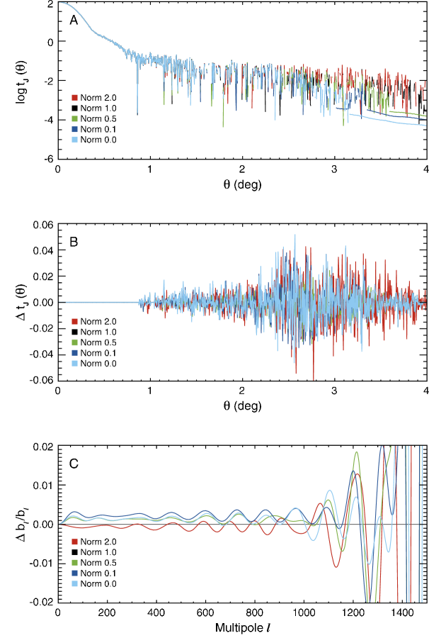
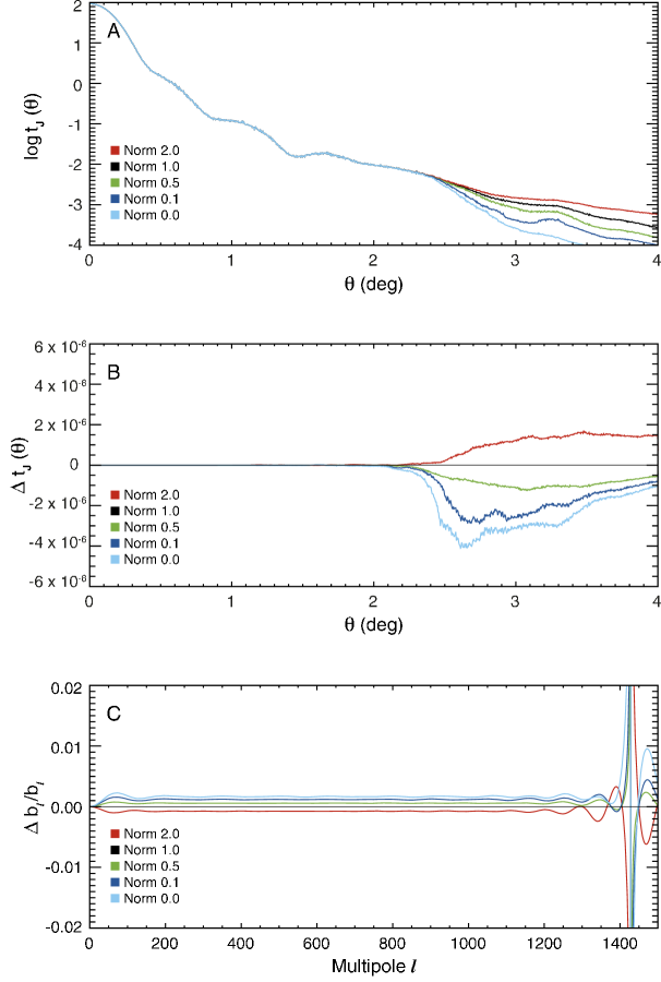
As described above (§2.3), the sidelobe data of the Moon motivate an attempt to augment the fitted distortions of the primary mirror ($k_{\mathrm{max}}=24$) with random distortions that are extrapolated to finer spatial scales, i.e., $k_{\mathrm{max}}=250$. These added distortions affect the hybridized beam through their effect on the outermost, low-gain part of the main beam model. One way of testing the effect of systematic error in the modeled beam tail is to rescale the extrapolated distortion amplitudes up or down as a group, with $100\%$ correlation. The resulting distortion amplitudes are used to compute new model beams, which are processed through hybridization with flight data and transformation to $b_{\ell}$.

The effect of this type of distortion rescaling on the beam transfer functions is shown in the bottom panel of Figure 8 for flight data, and Figure 9 for a noiseless simulation. Rescaling the added mirror distortions changes the slope of $b_{\ell}$ between $\ell=0$ and $\ell\sim 100$, while shifting $b_{\ell}$ up and down for $\ell\gtrsim 100$. Scale factors in the range $0-2$ result in a $\sim 0.3\%$ total range of variation in the high-$\ell$ value of $b_{\ell}$.

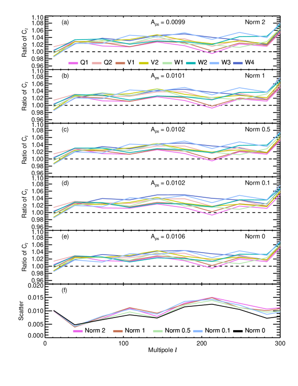
These scalings of the added distortions have been tested for their ultimate effect on CMB power spectra. Figure 10 shows the results of this test for scale factors of $2$, $1$, $0.5$, $0.1$, and $0$, respectively. Each panel shows a mean of year-by-year CMB cross power spectra computed from the five-year data set for each of the 8 WMAP DAs Q1–W4. The spectra are all computed using the MASTER estimator, and they are corrected for $b_{\ell}$ derived from augmented beams, characterized by distortion scale factors as indicated. For plotting, each such power spectrum is divided by the final MASTER power spectrum from the three-year WMAP analysis. In each case, a contribution from unresolved point sources is fitted and removed. In general, the result is that lower values of the scale factor give better consistency between microwave frequency bands for the CMB. Indeed, on this criterion, there is no clear reason to prefer a scale factor greater than zero.

As a result, the way the extrapolated random-phase mirror distortions are handled is by omitting them from the adopted beams and $b_{\ell}$, while the actual fitted mirror distortions with $k_{\mathrm{max}}\leq 24$ are retained, via the model part of the hybrid beam. However, we incorporate into the error analysis an estimate of the systematic error in the faint part of the model, by assuming that this error is of the same order as the adopted model, just as we do for optimizing $B_{\mathrm{thresh}}$ (§3.1). Monte Carlo experiments done on the primary mirror distortions suggest that this $100\%$ scaling error is conservative.

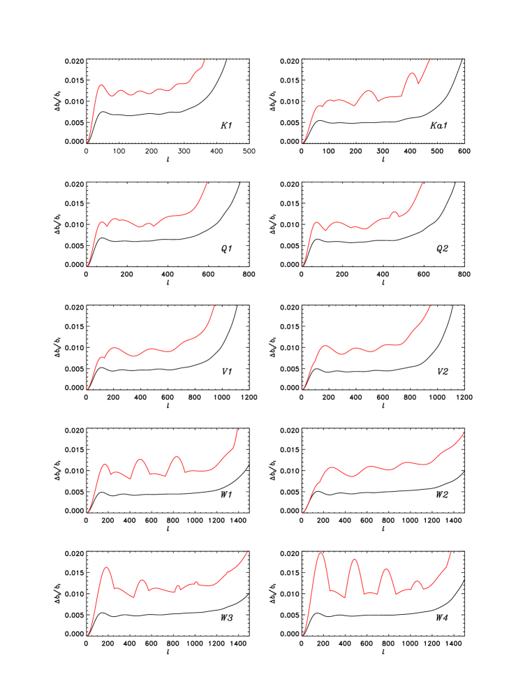
Combined errors in $b_{\ell}$, which arise both from observational scatter in the Jupiter measurements and from the scaling error in the model, are estimated using Monte Carlo simulations of the hybridization. The DADRA flight models are used to represent the true input beams. These models are sampled to match the observed beam positions in the five-year flight archive. Based on the chosen hybrization threshold, white noise is added to the model for the points that would be taken from Jupiter observations in the actual analysis. The model points that are substituted for the low-gain tail are multiplied by a common, normally distributed scaling factor with $\mu=\sigma=1$. Because the beam modeling is expected to be common mode across frequencies, the same scaling factor is used for every DA in a given Monte Carlo realization. A total of 5000 beam realizations is computed, each comprising all ten DAs. The beam transfer function is computed for each beam realization as described above for flight data, and the standard deviation of the realizations at each $\ell$ is used as the diagonal of the covariance matrix. Figure 11 shows the resulting error bands for each DA, compared to the adopted errors from the three-year analysis.

The chosen radial bin size of $0\farcm 25$ is the smallest width permitting all the bins to be populated. However, the bin sizes $0\farcm 5$ and $0\farcm 75$ have also been tested, in order to ensure that window function results are not affected. For the $\ell$ range of interest, the bin size contributes negligibly to the smearing of the beam, even in W band, and has no effect on the estimated error bars.

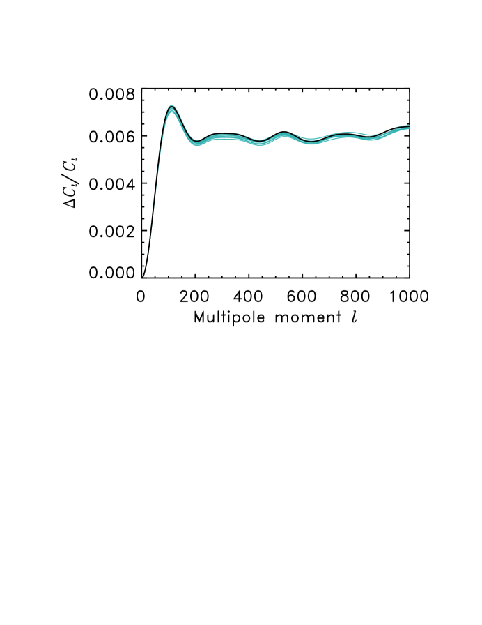
Monte Carlo realizations of $b_{\ell}$ for each DA are used in estimating the full covariance matrix of the coadded TT power spectrum in V and W. For CMB analysis, the error in the error is important. From several independent Monte Carlo runs of 5000 realizations apiece, the combined VW window function covariance has an error of $\sim\pm 3\%$ in the diagonal elements (Hinshaw et al., 2008). The beam-related errors in the coadded TT power spectrum are shown as a function of $\ell$ in Figure 12.

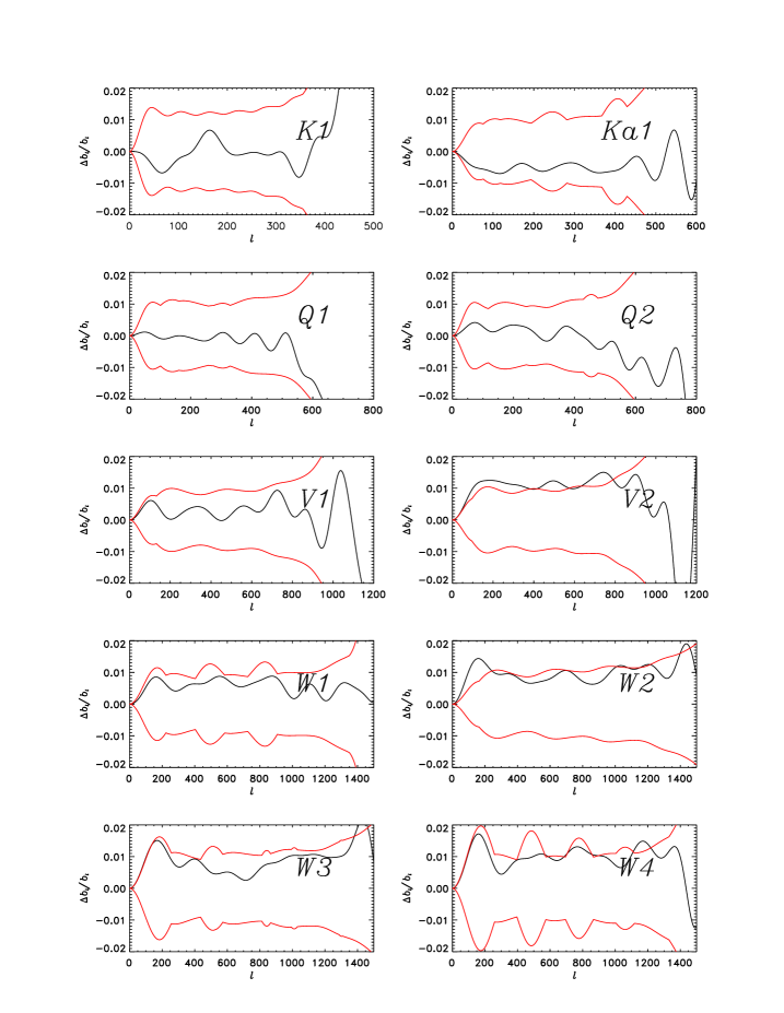
The comparison of three-year and five-year beam transfer functions is shown in Figure 13. Plotted is the relative change in $b_{\ell}$, i.e., $(b_{\ell}^{\mathrm{3yr}}-b_{\ell}^{\mathrm{5yr}})/b_{\ell}^{\mathrm{3yr}}$. Each beam is integrated out to the five-year transition radius; for this plot, the three-year beams are extended using the three-year sidelobe response patterns. Also plotted are $\pm 1\sigma$ errors of $b_{\ell}^{\mathrm{3yr}}$. The three-year and five-year $b_{\ell}$ are consistent, with $\sim 1\sigma$ changes in V2 and W1–W4. For these DAs, the change has the form of a plateau for $\ell\gtrsim 200$, reflecting an increase in the main beam solid angle for five years. This increase raises $B_{0}$ relative to $B_{200}$. The differences plotted in Figure 13 are taken with a sign convention reflecting the difference in the final power spectrum. Thus $\Delta b/b_{\ell}=1\%$ implies a $2\%$ change in $w_{\ell}$, in the sense that the high-$\ell$ power spectrum increases by $\sim 2\%$.

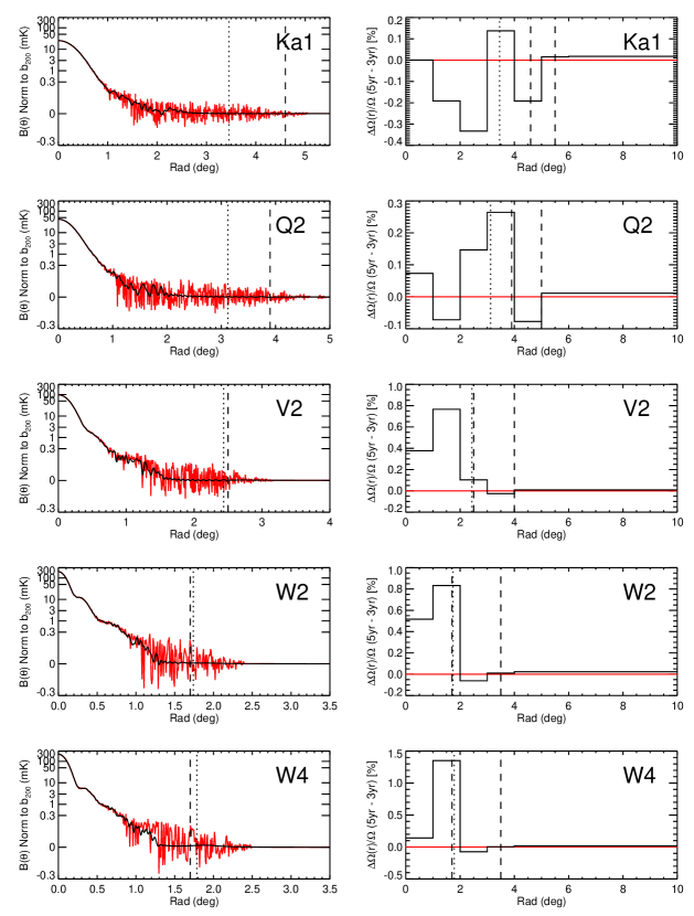
Solid angle changes are necessarily attributable to changes in the symmetrized beam profiles. Selected beam profiles are compared in the left column of Figure 14. The right column partitions the solid angle difference between five years ($\Omega_{B}^{\mathrm{5yr}}$) and three years ($\Omega_{B}^{\mathrm{3yr}}$) into $1\arcdeg$ radial bins. The contribution of each bin is plotted as a percentage of $\Omega_{B}^{\mathrm{5yr}}$. In this case, the beam profiles are extended to a radius of $10\arcdeg$ using the far sidelobe patterns. Also, solid angles are normalized in such a way as to equalize $b_{200}$ between the resulting three-year and five-year beam transfer functions. Most of the beam profile change, and therefore most of the solid angle change, is just inside the three-year transition radius (dashed line). Compare with Figure 4, which shows, for the pure model case, how the increase in the fitted $k_{\mathrm{max}}$ of the mirror distortions for five years of data increases the solid angle inside the three-year radius.

In summary, the solid angle increase appears to result primarily from the improved beam modeling, together with the extension of the main beam treatment to larger radii, both resulting from the increased $S/N$ of the Jupiter data. Optimally hybridized two-dimensional beams are symmetrized and reduced to radial profiles in an unbiased way by averaging in annuli, and the resulting profiles are transformed directly to $b_{\ell}$.

4 Radiometry of Planets Useful for Calibration

4.1 Jupiter

We adopt the analysis approach described in Page et al. (2003a) for reduction of the planet observations. The WMAP full-sky maps exclude observations made with Mars, Jupiter, Saturn, Uranus, or Neptune near any main beam boresight, with an exclusion radius of $1\fdg 5$. In turn, the sky maps are used to remove the background sky signal from planet data. Since the solid angle of each planet is much less than that of the WMAP beams, a beam map is built up by binning observed antenna temperatures for a planet in a focal plane coordinate system. Rather than being normalized, this beam map may be left in antenna temperature and Legendre transformed (Eq. 4) to produce an unnormalized beam transfer function, $T_{\mathrm{J}}^{m}B_{\ell}$, where $T_{\mathrm{J}}^{m}$ is the peak antenna temperature of Jupiter. But $B_{0}$ is the beam solid angle $\Omega_{B}$, so that $T_{\mathrm{J}}^{m}B_{0}=T_{\mathrm{J}}^{m}\Omega_{B}$ (Page et al., 2003a), and $T_{\mathrm{J}}^{m}B_{0}/\Omega_{\mathrm{J}}^{\mathrm{ref}}=T_{\mathrm{J}}$, where $T_{\mathrm{J}}$ is the brightness temperature of the Jupiter disk, and $\Omega_{\mathrm{J}}^{\mathrm{ref}}$ is the fiducial solid angle $2.481\times 10^{-8}$ sr for a Jupiter–WMAP distance of 5.2 AU (Griffin et al., 1986). The error in $T_{\mathrm{J}}$ is then the sum in quadrature of the error in $\Omega_{B}$ with the estimated WMAP gain calibration error of $0.2\%$ (Hinshaw et al., 2008). The results of this procedure are given in Table 5 for five years of Jupiter data in each DA.

The main difference between the Legendre transform method and a direct integration of the two-dimensional beam map is that the Legendre transform uses a symmetrized beam profile. Integration of the beam map yields solid angles within the errors of the above approach. The results in Table 5 are consistent with the band averaged ones previously reported by Page et al. (2003a, §2.4). Currently, the error in $T_{\mathrm{J}}$ is limited by the $0.5\%$ error in beam solid angle and the $0.2\%$ gain uncertainty.

Season-by-season radiometry of Jupiter is given in Table 6. The values are computed using a template-fitting technique. Radial profiles are produced for each DA for each Jupiter season, then fitted linearly against the mean five-year Jupiter radial profile. Season 2 is omitted because Jupiter is approaching the Galactic anticenter, making background subtraction problematic. Our data place an upper limit on the time variability of $T_{\mathrm{J}}$ as a function of orbital phase of $0.3\%\pm 0.5\%$. We conclude that our radiometric observations are consistent with the absence of variability in the Jupiter brightness temperature at this level.

In view of the stability and low errors of these measurements, Jupiter radiometry is the preferred method of transferring the WMAP dipole calibration to another microwave instrument. The key requirement for such an effort is knowledge of the beams. The error values given in Table 5 include WMAP beam errors via error in solid angle, as well as the fundamental gain uncertainty relative to the dipole.

4.2 Other Planetary Calibrators

Millimeter-wave brightnesses of other planets are also of potential interest as calibrators. For example, for the WMAP W band beams ($3.2$ mm), peak antenna temperatures of $\sim 200$ mK, $\sim 35$ mK, and $\sim 6$ mK are produced by Jupiter, Saturn, and Mars, respectively. A preliminary analysis of the WMAP five-year Mars and Saturn observations has been undertaken.

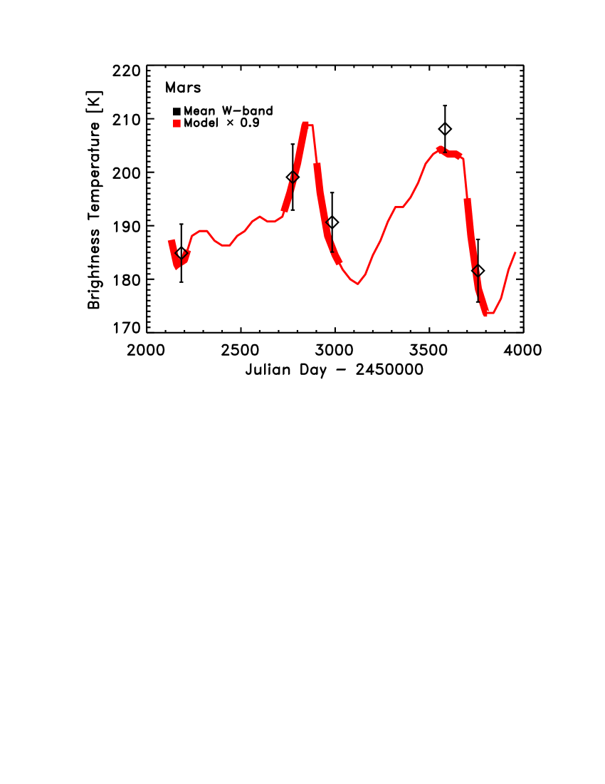
Mars is attractive as a calibration source because it is relatively bright. However, significant variations in the observed brightness temperature can occur because of the viewing geometry. Moreover, the radiating properties of the inhomogeneous, pitted planetary surface complicate the determination of an appropriate reference brightness. Figure 15 shows a thermal model developed for the infrared by Wright (1976, 2007). The model is evaluated at $3.2$ mm (W band) as a function of the time within the WMAP five-year timeline, which includes five Mars observing seasons (fewer than for Jupiter because of the relative orbital velocity of Mars). The predicted variation in brightness temperature over an observing season can be as much as $\sim 20$ K. The mean $3.2$ mm temperature and the scatter among the four W DAs are also shown for WMAP data binned by Mars observing season (Table 7). The model is higher than the WMAP measurements by $\sim 10\%$, so that a renormalization factor of $0.9$ is applied to the model in the plot. We use this Mars model partly because of its previous use for Earth-based infrared calibration and the convenient availability of the code (Wright, 2007); for a model including the effects of a dusty atmosphere and polar caps, see Simpson et al. (1981). The Mars data are referenced to a fiducial distance of $1.5$ AU and a solid angle of $\Omega_{\mathrm{Mars}}^{\mathrm{ref}}=7.156\times 10^{-10}$ sr (Hildebrand et al., 1985).

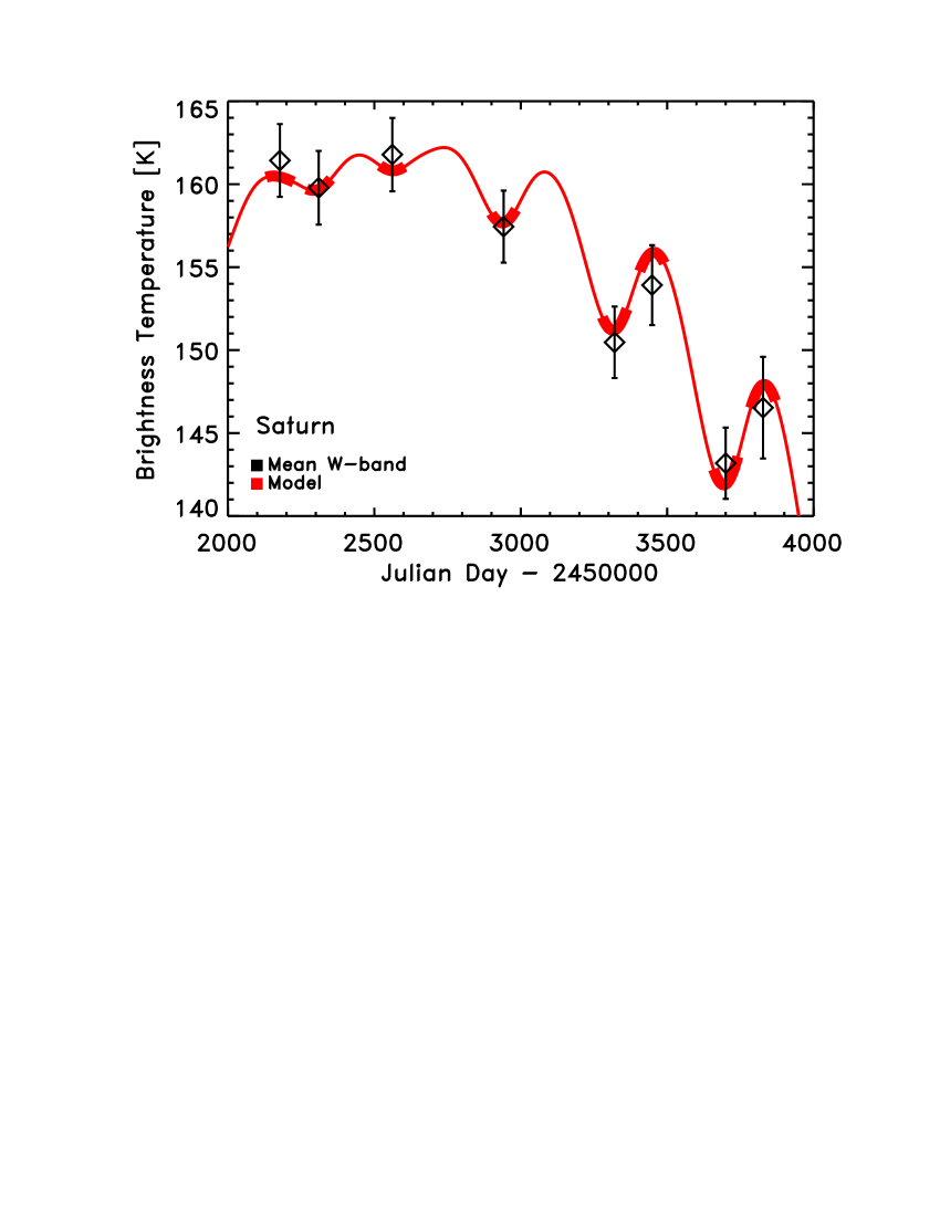
Saturn’s apparent brightness is even greater than that of Mars, but the theoretical understanding of the radiometry is less developed (Ulich, 1981; Epstein et al., 1980; Hildebrand et al., 1985). A special consideration is Saturn’s ring system, of which the viewing aspect from the Earth changes over the course of Saturn’s 29 year orbital period. In Figure 16, mean seasonal W-band brightness temperatures as measured by WMAP (Table 7) are shown as black diamonds. These data show a clear decrease in observed temperature with time, a trend which correlates extremely well with the decreased viewing cross-section of Saturn’s rings in the same time interval. A simple model of the form $T_{\mathrm{Sat}}=T_{0}+\alpha\sin i$, where $i$ is the inclination of the ring plane from our line of sight, is fitted to the data and plotted in red. The fit results are $\alpha=-132\pm 16$ and $T_{0}=102\pm 7$. Possible physical causes for the temperature decrease include the decreasing projected radiating area of the rings, a less favorable viewing angle for the “hot spot” at the south pole of Saturn, and Saturn’s oblateness. These causes will be the subject of future investigation. The Saturn data are referenced to a fiducial distance of $9.5$ AU, corresponding to a Saturn solid angle of $\Omega_{\mathrm{Sat}}^{\mathrm{ref}}=5.101\times 10^{-9}$ sr (Hildebrand et al., 1985).

Clearly, Jupiter remains the only WMAP source that can be recommended as an instrument calibrator at the $1\%$ level. However, our preliminary results for Mars and Saturn suggest that with additional analysis and observations, both of these sources may be similarly useful in the future.

5 Conclusions

WMAP observes the planet Jupiter in two seasons a year, each of $\sim 50$ days. Ten seasons of Jupiter observations are used in this paper to measure the in-flight beam patterns associated with each of the multifrequency WMAP radiometers. An accurate beam pattern determination is critical for cosmological measurements.

Using the TOD, beam maps are formed from the Jupiter observations for both the A-side and B-side optics. The A-side fitting is improved over previous analyses both by additional data and by extension of our analysis techniques. The B side is now directly fitted for the first time. The cutoff scale length of fitted primary mirror distortions is reduced from previous analyses by a factor of $\sim 2$. The hybridization of beam models with beam data is optimized explicitly with respect to error in the main beam solid angle. We transform the hybridized, symmetrized main beam profiles into harmonic space without an intermediate spatial fitting function.

Although the beam transfer functions are statistically consistent with earlier ones, a $\sim 1\%$ increase in solid angle is found for the V2 and W1–W4 DAs because of improved data and refinement of previous analysis methods. The uncertainty in the beam transfer functions is decreased by a factor of $\sim 2$ relative to previous WMAP beam analyses, demonstrating the success of continued mission operations and continued progress from data analysis efforts. Extended operations and analysis will further reduce these uncertainties.

Table 1: Abbreviated Fit History for Side A

Primary	Primary	Secondary
$k_{\mathrm{max}}$	Modes	Modes	$\chi_{\nu}^{2}$
12	122	30	1.15
14	158	30	1.17
16	206	30	1.11
18	262	30	1.11
20	326	30	1.12
22	386	30	1.11
24	450	30	1.05

Table 2: Abbreviated Fit History for Side B

Primary	Primary	Secondary
$k_{\mathrm{max}}$	Modes	Modes	$\chi_{\nu}^{2}$
4	22	0	2.50
6	38	9	1.26
6	38	30	1.27
8	58	30	1.22
10	90	30	1.17
12	122	30	1.17
14	158	30	1.16
16	205	30	1.15
18	262	30	1.15
20	326	30	1.15
22	386	30	1.11
24	450	30	1.07

Table 3: Main Beam Limits

	3-Year Radius	5-Year Radius	3-Year $B_{\mathrm{thresh}}$	5-Year $B_{\mathrm{thresh}}$	$r_{50}$
DA	($\arcdeg$)	($\arcdeg$)	(dBi)	(dBi)	($\arcdeg$)
K1	6.1	7.0	17	3	4.3
Ka1	4.6	5.5	17	4	3.5
Q1	3.9	5.0	18	6	3.1
Q2	3.9	5.0	18	6	3.1
V1	2.5	4.0	19	8	2.5
V2	2.5	4.0	19	8	2.4
W1	1.7	3.5	20	11	1.8
W2	1.7	3.5	20	11	1.7
W3	1.7	3.5	20	11	1.7
W4	1.7	3.5	20	11	1.8

Table 4: Main-Beam Solid Angles, Gains, and $\Gamma$ for Combined Maps

	$\Omega^{S}$	$\Delta(\Omega^{S})/\Omega^{S}$	$G_{m}$	$\Gamma_{\mathrm{ff}}$
DA	(sr)	(%)	(dBi)	($\mu$K Jy-1)
For 10 Maps
K1	$2.447\times 10^{-4}$	0.7	46.97	262.2
Ka1	$1.436\times 10^{-4}$	0.5	49.41	211.8
Q1	$8.840\times 10^{-5}$	0.6	51.40	222.8
Q2	$9.145\times 10^{-5}$	0.6	51.29	216.6
V1	$4.169\times 10^{-5}$	0.4	54.85	214.1
V2	$4.240\times 10^{-5}$	0.4	54.75	205.7
W1	$2.037\times 10^{-5}$	0.4	57.97	184.7
W2	$2.206\times 10^{-5}$	0.4	57.67	168.7
W3	$2.149\times 10^{-5}$	0.5	57.77	176.6
W4	$1.998\times 10^{-5}$	0.5	57.95	186.7
For 5 Maps
K	$2.447\times 10^{-04}$	0.7	46.97	262.7
Ka	$1.436\times 10^{-04}$	0.5	49.41	211.9
Q	$8.993\times 10^{-05}$	0.6	51.34	219.6
V	$4.204\times 10^{-05}$	0.4	54.80	210.1
W	$2.098\times 10^{-05}$	0.5	57.84	179.2

Table 5: Five-Year Mean Jupiter Temperatures

DA	$\nu_{e}^{\mathrm{RJ}}$	$T$	$\sigma(T)$
	(GHz)	(K)	(K)
K1	22.8	135.2	0.93
Ka1	33.0	146.6	0.75
Q1	40.9	154.7	0.96
Q2	40.9	155.5	0.94
V1	61.0	165.0	0.80
V2	61.6	166.3	0.77
W1	93.8	172.3	0.78
W2	94.1	173.4	0.82
W3	93.2	174.4	0.87
W4	94.1	173.0	0.86

Table 6: Jupiter Temperature Changes by Season

Season	Start	End	$\Delta T/T$ (%)		$r/\overline{r}$
			Mean	Scatter
1	2001/10/08	2001/11/22	0.16	0.12	0.96
3	2002/11/10	2002/12/24	$-0.14$	0.23	0.97
4	2003/03/15	2003/04/29	$-0.25$	0.49	0.99
5	2003/12/11	2004/01/23	$-0.02$	0.24	1.00
6	2004/04/15	2004/05/30	$-0.01$	0.30	1.01
7	2005/01/09	2005/02/21	0.03	0.19	1.02
8	2005/05/16	2005/07/01	0.01	0.27	1.02
9	2006/02/07	2006/03/24	0.05	0.19	1.02
10	2006/06/16	2006/08/02	0.08	0.35	1.02

Table 7: W-Band Observations of Mars and Saturn

Julian Day	$T_{\mathrm{planet}}$	Scatter
$-2450000$	(K)	(K)
Mars
2184	185	5.4
2775	199	6.2
2984	191	5.6
3583	208	4.4
3758	182	5.9
Saturn
2178	161	2.2
2310	160	2.2
2562	162	2.2
2942	157	2.2
3321	150	2.2
3449	154	2.4
3700	143	2.2
3828	147	3.1

Figure 1: Flow chart of beam and window function processing. Boxes are color coded as follows: green, starting data; pink, intermediate data; blue, computations or processing steps; magenta, the result, $b_{\ell}$, which is the beam transfer function. The window function, $w_{\ell}$, for power spectra $C_{\ell}$ involving a single DA, is $b_{\ell}^{2}$. Dashed boxes enclose iterative algorithms.

Figure 2: Beams in the WMAP focal plane for side A (left) and side B (right). The top panels show the measured beams, the middle panels show the beam models, and the bottom panels show the residuals. In the top four panels, each beam is scaled to its maximum (red) and plotted logarithmically to a level of $-40$ dB (blue). For the bottom panels, each beam’s residual is shown linearly as 100(data$-$model)/beam peak. The scales are $\pm 10\%$ for K1; $\pm 5\%$ for Ka1, Q1, and Q2; $\pm 3\%$ for V1 and V2; and $\pm 2.5\%$ for W1–W4. A similar depiction of the A side only for three years of data is in Figure 9 of Jarosik et al. (2007).

Figure 3: Fitted distortions of the A-side (left) and B-side (right) mirrors with respect to nominal shapes. $Y$ axis is negative in the sky direction and positive toward the main spacecraft structure. Top row: primary mirrors. The dominant feature of the primary mirror distortions is the central rectangle, corresponding to a frame that is part of the backing structure. Hints of the stiffening lugs in the backing structure may also be seen around the edges. Bottom row: secondary mirrors. The mirrors are constrained only where they are substantially illuminated by the feed horns (Page et al., 2003b). Thus, for example, the secondary mirror for the B side appears as a bull’s-eye partly because the fit is only constrained near the center. Gray line: contour of the mean W band illumination function $-15$ dB from the peak. Although the mirrors are elliptical in outline, these plots are circular. The reason is that the distortions are parametrized as displacements along the axis of a circular cylinder containing the mirror boundary.

Figure 4: Growth of solid angle in model beams as a function of $k_{\mathrm{max}}$, for the V2 DA on the A side. Top: logarithmically scaled images of the model beam pattern as fitted for $k_{\mathrm{max}}=12$, 14, 16, 18, 20, 22, and 24, respectively, together with a beam that combines the $k_{\mathrm{max}}=24$ fit with random-phase modes extrapolated to $k=250$. Axis tick marks are at $1\arcdeg$ intervals. Bottom left: azimuthally averaged beam profiles for the models pictured, in units of gain relative to isotropic. Indigo–red: profiles of the seven beam models from $k_{\mathrm{max}}=12$ through $k_{\mathrm{max}}=24$, respectively. Gray: $k_{\mathrm{max}}=250$ extrapolation result. Black: Upper limit on the main beam sensitivity from Moon observations, obtained for side A by integrating over positive pixels in the differential sidelobe response pattern. The five-year model tail, which is a feature of the two-dimensional beam pattern, is the part of the beam that is both inside the transition radius and below the hybridization threshold (dotted line; see §3.3). The hybridization threshold and transition radius from the three-year analysis are indicated by the dashed line. Bottom right: model tail solid angle as a function of $k_{\mathrm{max}}$, relative to the total solid angle inside the transition radius; squares, five-year; triangles, modified tail of five-year models, using three-year threshold and transition radius. Fitting to $k_{\mathrm{max}}=24$ rather than $k_{\mathrm{max}}=12$ increases by a factor of $\sim 2$ the solid angle of the model tail as defined by three-year main beam limits. But note that the difference between the various fits is $\sim 0.1\%$ of the total beam solid angle for the 5 year data.

Figure 5: Power spectra of A-side (top) and B-side (bottom) primary mirror distortions as a function of spatial frequency on the primary mirror surface, $f=k/(280\ \mathrm{cm})$, where $k$ is the spatial frequency index used in the physical optics fits. Vertical bars on the $f$ axis indicate $f$ corresponding to $k=12$ and $k=24$. Solid lines: extrapolated power-law distortion spectra with slopes fitted by comparison to Moon sidelobe data, namely, $\alpha=4.95$ for the A side and $\alpha=4.43$ for the B side. In practice, these extrapolated distortions are used to update the sidelobe response patterns, but not to model the main beams. The error bars and upper limits show the mean absolute deviation about the mean of points with length scales less than $15$ cm, indicated by the dotted vertical line. Dashed curves: power spectra of primary mirror distortions from ground-based laboratory measurements of the surface, assuming a Gaussian form for the two-point correlation function, with correlation length 9.3 cm for the A side and 11.3 cm for the B side; normalized to points with $f<0.05$ cm^-1 (top) and $f<0.04$ cm^-1 (bottom).

Figure 6: A-side augmented beam profiles (green) compared to Moon sidelobe data (red). K1 and Ka1 appear to be dominated by diffuse reflection rather than the extended main beam, and so are excluded from the fit. Conspicuous DA-to-DA differences are seen in the quality of the fit, e.g., W1 and W2 as compared to V1 and V2. Contamination of the fit by diffuse reflected light cannot be ruled out even in DAs other than K1 and Ka1; thus, the Moon data are best considered as upper limits. Vertical line: maximum radius of Moon data included in fit, for DAs Q1–W4.

Figure 7: Fractional error in hybrid beam solid angle as a function of hybridization threshold, for the V2 DA. As the hybridization threshold is raised, noisy Jupiter data are excluded, so that the Jupiter data uncertainty (red) falls. At the same time, the model uncertainty (blue), estimated as a scaling error of $100\%$, increases because more of the two-dimensional model beam is used. These contrary slopes produce a well-defined minimum in the total error (green). Hybridization threshold values for the five-year analysis are chosen near the location of this minimum, as shown by the vertical line. Plots for other DAs are similar. The adopted thresholds are rounded to an even dBi unit and are constant for each frequency band, as shown in Table 3.

Figure 8: (Top) Symmetrized radial profiles of hybridized, binned flight beams for the V2 DA. The central, high $S/N$ part of the beam is taken directly from flight data of the planet Jupiter, whereas the part of the beam below a given gain cutoff is taken from beam models. The set of beam models shown comprises several normalizations of the extrapolated primary-mirror distortions; the normalization favored in the analysis is zero, meaning that the extrapolated distortions are omitted. The noise-free lines at radii $3\arcdeg-4\arcdeg$ are portions of the lower-normalization profiles that include model points only. (Middle) Same profiles as in the top panel, after subtraction of the one with normalization 1.0. (Bottom) Beam transfer functions corresponding to the depicted beam profiles, relative to the one with normalization 1.0. Cf. Figure 9, especially the bottom panel. The beam transfer functions at $\ell\gtrsim 100$ are close to what is expected from the noise-free simulations, implying good solid angle recovery.

Figure 9: (Top) Radially binned noise-free simulations of hybridized beams for the V2 DA. The central part of the beam is taken from the adopted DADRA model without augmented distortions. The part of the beam below a given gain cutoff is taken from augmented beam models with various normalizations of the extrapolated primary-mirror distortions. The analysis of hybrid beams including real Jupiter data favors the zero normalization, meaning that the extrapolated distortions are omitted. (Middle) Same profiles as in the top panel, after subtraction of the one with normalization 1.0. (Bottom) Beam transfer functions corresponding to the depicted beam profiles, relative to the one with normalization 1.0. Fits using flight hybrid beams should approximate the curves shown here.

Figure 10: Consistency of CMB power spectra across frequency bands, for window functions derived from various normalizations of the extrapolated primary mirror distortions. Complete omission of such extrapolated distortions from the main beam model is justified by this criterion. The CMB spectra and unresolved point-source coefficients ($A_{\mathrm{ps}}$) in this plot are from a preliminary stage of analysis and are not the final five-year WMAP results. (a)-(e): Mean of year-to-year cross spectra in each DA, relative to the final combined power spectrum from the three-year analysis. The applied $w_{\ell}$ are derived from hybridized beams in which the tail is from a beam model with extrapolated primary mirror distortions; hybridization thresholds in each DA optimize solid angle error for the nominal amplitude of these added distortions (Figure 5). Spectrum is binned in $\ell$ with a bin size of $\Delta\ell=35$. The panels differ in the scaling of the extrapolated distortion amplitude on the mirror: (a), 2; (b), 1; (c), 0.5; (d), 0.1; (e) no extrapolated distortions. (f) Scatter among the DAs in each $\ell$ bin for the five normalizations of the extrapolated mirror distortions. Omitting the extrapolated distortions (Norm 0, black) minimizes the scatter in the CMB power spectrum over most of this $\ell$ range, which includes the first peak near $\ell\sim 200$.

Figure 11: Relative error in beam transfer functions ($\Delta b_{\ell}/b_{\ell}$) for the five-year beams (black) vs. the three-year errors (red) (Jarosik et al., 2007). The five-year uncertainties are typically a factor of $\sim 2$ better than three-year uncertainties.

Figure 12: Relative error component that is due to estimated beam errors in the final WMAP TT power spectrum, which is combined from V and W band data. Cyan: eight independent instances of the square root of the diagonal of the covariance matrix for the coadded VW $C_{\ell}$; each instance is based on 5000 Monte Carlo realizations of V and W beam errors. Black: the instance that has been chosen for the $C_{\ell}$ error bar, because it is approximately the upper envelope.

Figure 13: Consistency within $\sim 1\sigma$ of five-year beam transfer functions with three-year beam transfer functions. Black: difference of three-year minus five-year $b_{\ell}$, relative to the five-year $b_{\ell}$; the low-$\ell$ rise or fall for several DAs reflects solid angle changes detailed in Figure 14. Red: three-year $1\sigma$ errors. For this plot, the beam profiles used to compute $b_{\ell}$ are extended by including the profile of the inner portion of each sidelobe response pattern, and the resulting composite profiles are integrated out to the five-year transition radii. This removes the effect of the larger five-year transition radius.

Figure 14: Much of the solid angle change between the three-year and five-year beams arises inside the three-year main-beam boundaries. In this figure, the beam profiles are extended to a radius of $10\arcdeg$ using the three-year or five-year sidelobe response pattern, respectively, and the beams are normalized to give the same $b_{200}$ for both three years and five years. Solid angle changes by $|\Delta\Omega_{B}|/\Omega_{B}<0.5\%$ for the K1, Ka1, Q1, Q2, and V1 DAs, and by $0.8\%\leq\Delta\Omega_{B}/\Omega_{B}\leq 1.5\%$ for the V2 and W1–W4 DAs. Left: Five-year symmetrized hybrid beam profiles (red) and three-year Hermite-fitted beam profiles (black) for selected DAs. The five-year profiles include Jupiter data and so are noisy, whereas the three-year profiles are the functional fit only. Dashed line: three-year transition radius (Table 3). Dotted line: radius where five-year hybrid beams consist of $50\%$ data and $50\%$ model. Right: Change in beam solid angle from the three- to the five-year analysis, as a function of radius, in annuli of $1\arcdeg$, expressed as a percentage of the five-year $\Omega_{B}$. Dashed lines: Transition radii for three years and five years, respectively. Dotted lines: $50\%$ data radius of hybrids, as in left column.

Figure 15: Comparison of WMAP observations (Table 7) to the Mars brightness model of Wright (1976, 2007), evaluated at a wavelength of $3.2$ mm (W band). Mean WMAP meaurements are shown for each observing season (diamonds), with error bars indicating the scatter among WMAP DAs W1–W4. Model values (red) are rescaled by $0.9$ to bring them into overall agreement with the measurements; thick portions of the line indicate observing seasons. WMAP data are referenced to a fiducial distance of $1.5$ AU and a solid angle of $\Omega_{\mathrm{Mars}}^{\mathrm{ref}}=7.156\times 10^{-10}$ sr (Hildebrand et al., 1985). There are significant variations in the observed brightness temperature due to both geometric and physical factors, and thus, some care must be exercised before taking Mars as a calibration source.

Figure 16: Season-by-season WMAP radiometry of Saturn in the W band (Table 7). Diamonds: Mean WMAP measurements for each of eight observing seasons, with error bars indicating the scatter among WMAP DAs W1–W4. WMAP data are referenced to a fiducial distance of $9.5$ AU, corresponding to a Saturn solid angle of $\Omega_{\mathrm{Sat}}^{\mathrm{ref}}=5.101\times 10^{-9}$ sr (Hildebrand et al., 1985). Red line: simple fitting model of the form $T_{\mathrm{Sat}}=T_{0}+\alpha\sin i$, where $i$ is the inclination of the ring plane from our line of sight. Thick portions of the line indicate observing seasons. Fitted parameters are $\alpha=-132\pm 16$ and $T_{0}=102\pm 7$. Although the model appears to capture geometric aspects of the observations surprisingly well, it lacks the physical underpinning to be used predictively.

References

- Barnes et al. (2003) Barnes, C., et al. 2003, ApJS, 148, 51
- Bennett et al. (1992) Bennett, C. L., et al. 1992, ApJ, 391, 466
- Bennett et al. (2003) —. 2003, ApJ, 583, 1
- Epstein et al. (1980) Epstein, E. E., Janssen, M. A., Cuzzi, J. N., Fogarty, W. G., & Mottmann, J. 1980, Icarus, 41, 103
- Griffin et al. (1986) Griffin, M. J., Ade, P. A. R., Orton, G. S., Robson, E. I., Gear, W. K., Nolt, I. G., & Radostitz, J. V. 1986, Icarus, 65, 244
- Gorski et al. (2005) Gorski, K. M., Hivon, E., Banday, A. J., Wandelt, B. D., Hansen, F. K., Reinecke, M., & Bartlemann, M. 2005, ApJ, 622, 759
- Hildebrand et al. (1985) Hildebrand, R. H., Loewenstein, R. F., Harper, D. A., Orton, G. S., Keene, J., & Whitcomb, S. E. 1985, Icarus, 64, 64
- Hinshaw et al. (2007) Hinshaw, G., et al. 2007, ApJS, 170, 288
- Hinshaw et al. (2008) Hinshaw, G. et al. 2008, ApJS, submitted
- Jarosik et al. (2007) Jarosik, N., et al. 2007, ApJS, 170, 263
- Limon et al. (2008) Limon, M., et al. 2008, Wilkinson Microwave Anisotropy Probe (WMAP): Explanatory Supplement, http://lambda.gsfc.nasa.gov/data/map/doc/MAP_supplement.pdf
- Nolta et al. (2008) Nolta, M. R. et al. 2008, ApJS
- Page et al. (2003a) Page, L., et al. 2003a, ApJS, 148, 39
- Page et al. (2003b) Page, L., et al. 2003b, ApJ, 585, 566
- Rahmat-Samii et al. (1995) Rahmat-Samii, Y., Imbriale, W., & Galindo-Isreal, V. 1995, DADRA, YRS Associates, rahmat@ee.ucla.edu
- Simpson et al. (1981) Simpson, J. P., Cuzzi, J. N., Erickson, E. F., Strecker, D. W., & Tokunaga, A. T. 1981, Icarus, 48, 230
- Standish (1990) Standish, Jr., E. M. 1990, A&A, 233, 252
- Ulich (1981) Ulich, B. L. 1981, AJ, 86, 1619
- Wright (1976) Wright, E. L. 1976, ApJ, 210, 250
- Wright (2007) —. 2007, preprint (astro-ph/0703640)
- Wright et al. (2008) Wright, E. L. et al. 2008, ApJS, submitted