The growth of matter perturbations in some scalar-tensor DE models
We consider asymptotically stable scalar-tensor dark energy (DE) models for which the equation of state parameter tends to zero in the past. The viable models are of the phantom type today, however this phantomness is milder than in General Relativity if we take into account the varying gravitational constant when dealing with the SNIa data. We study further the growth of matter perturbations and we find a scaling behaviour on large redshifts which could provide an important constraint. In particular the growth of matter perturbations on large redshifts in our scalar-tensor models is close to the standard behaviour , while it is substantially different for the best-fit model in General Relativity for the same parametrization of the background expansion. As for the growth of matter perturbations on small redshifts, we show that in these models the parameter can take absolute values much larger than in models inside General Relativity. Assuming a constant when is large would lead to a poor fit of the growth function . This provides another characteristic discriminative signature for these models.
PACS Numbers: 04.62.+v, 98.80.Cq
1 Introduction
The aim of Dark Energy models is to explain the late-time accelerated expansion of the universe [1]. Like for inflationary models producing an early stage of accelerated expansion, we have now a wide variety of DE models that can account for the late-time background evolution [3]. In the same way that inflationary models are constrained by the cosmological perturbations they produce, DE models can be constrained by the background evolution and their effect on the growth of perturbations. In principle what is basically needed is a smooth component with a sufficiently negative pressure. Among DE models, CDM, although it contains a cosmological constant which can be seen as “unnaturally” small, is the simplest model and this model is presently in good agreement with observations on large scales (see however e.g.[4]). Another class of appealing models are quintessence models containing a minimally coupled scalar field [5]. A possible drawback of these models is their inability to violate the weak energy condition and to account for a phantom phase. Many more models of ever increasing sophistication have been proposed [6]. To make progress, it is important to find ways to select those classes of DE models that remain observationnally viable and to find characteristic signatures that will enable us to constrain them, or even rule them out, with more accurate data at our disposal in the future.
In particular, an interesting family of DE models are those where gravity is no longer described by General Relativity (GR). Indeed there has been considerable interest recently in DE models with gravitation modified with respect to General Relativity, a feature that is quite generic in higher dimensional theories or also in the low energy effective action of more fundamental four-dimensional theories. Well-motivated models belonging to this class which can be explored thoroughly are scalar-tensor dark energy models [7, 8, 9, 10, 11]. Like the usual quintessence models containing a minimally coupled scalar field, scalar-tensor models have an additional physical degree of freedom, namely the scalar partner of the graviton. However, these models are more complicated as they have two free fundamental functions in their lagrangian, one more function in addition to the scalar field potential. This additional function reflects the modification of gravity encoded in the theory. A generic feature of these models, like for essentially all alternatives to the cosmological constant model, is that DE has a time-varying equation of state. The fact that CDM fits well a large amount of observations should be an incentive to look for models with time-varying equation of state still able to compete with CDM.
As for all DE models, scalar-tensor DE models are characterized by the accelerated expansion they produce at low redshifts but this background effect is common to all DE models. The modification of gravity with respect to General Relativity is more specific and it expresses itself in particular in the modified growth of linear cosmological matter perturbations. In this way, under quite general asumptions, it could be possible to determine from the growth of matter perturbations combined with the background expansion whether a DE model lies inside General Relativity or not [12, 13] (see also [14]). Hence it is very important to investigate how this can be extracted from the observations [15, 16]. Scalar-tensor DE models are certainly good examples to investigate this issue. Aside from deeper theoretical motivations, an additional incentive to consider scalar-tensor models could come from the observations if these support DE models which have a phantom phase (see also [17] for other models that can produce a phantom phase).
We will consider asymptotically stable, internally consistent, scalar-tensor DE models [10]. For such models = constant and asymptotic stability is possible for and . We can consider varying equations of state provided . As we will show these models exhibit a characteristic signature in the growth of matter perturbations on large and on small redshifts. This could potentially allow us to constrain them or even rule them out. In connection with the growth of matter perturbations on small redshifts, these models will illustrate results derived in an earlier work [18], namely the possibility to have a parameter whose absolute value is much larger than in General Relativity when we write the growth factor as . Indeed, it was shown in [10] that in models with a constant or a (smoothly) varying equation of state inside GR and hence also for CDM. On the other hand, on large redshifts there can also be an important effect on the growth of perturbations. Interestingly, as we will see, we can have models for which the growth of matter perturbations on large scales is close to that in CDM and for which the growth of matter perturbations deviates most from that in CDM on small redshifts. Another interesting aspect of a varying gravitational constant is its effect on the interpretation of SNIa data and we will show that less phantomness is required today by the observations for our models compared to General Relativity. Indeed as we consider DE models where in the past, a large amount of phantomness is required by the observations if we are inside GR while in our models this is much less the case.
2 An asymptotically stable scalar-tensor model
It is important to review here the basic aspects and definitions of our scalar-tensor models. We consider DE models where gravity is described by the Lagrangian density in the Jordan (physical) frame
| (1) |
The Brans-Dicke parameter is given by where a prime denotes a derivative with respect to redshift , and
| (2) |
Specializing to a spatially flat universe, the DE energy density and pressure are defined as follows
| (3) | |||||
| (4) |
With these definitions, the usual conservation equation applies:
| (5) |
With the equation of state parameter defined through
| (6) |
the time evolution DE obeys the usual rule
| (7) |
Equations (3) can be rewritten as
| (8) |
where by definition as we assume a spatially flat universe. For these models
| (9) |
hence the weak energy condition for DE can be violated ([10], see also [19]).
We consider viable models satisfying the following requirements:
1) for .
2) The DE equation of state evolves according to for .
3) Consistency requires .
4) We impose .
Condition 1) is reminiscent of the models considered in [20]. For these models we have that = constant from some redshift on, and different from one by a few percents only. In order to have accelerated expansion at the present time we need some dynamical DE equation of state. We consider a parametrization [21],[22] with a smoothly varying equation of state where DE tends to a scaling behaviour in the past
| (10) |
where . If we impose for , this prameterization reduces to the simple form
| (11) |
The corresponding DE evolution reads [21]
| (12) |
For given cosmological parameters and the background evolution is completely fixed by the parameter . We have in particular
| (13) |
Clearly,
| (14) |
The quantity is fixed by and . As shown in [10], the requirement 1) implies the inequality (independent of the specific form of )
| (15) |
In particular a large amount of phantomness today implies close to one and hence close to . We use further the following ansatz
| (16) |
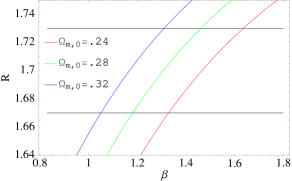
This ansatz satisfies exactly while . For the ansatz (16), we must have in addition which comes from the requirement at . So we impose the functions and from which all other quantities can be reconstructed and we check the physical consistency for each reconstructed scalar-tensor model. As is imposed, so is the background dynamics. In this way we can compare different DE models inside and outside General relativity possessing the same background evolution. Clearly, as the DE equation of state parameter tends to zero as increases, it must start being phantom today if it is to pass the observational constraints. This can be seen more quantitatively using the constraint on the shift parameter. We see from Figure 1 that the viable models are of the phantom type today (). The possibility to have a phantom DE sector today is actually an attractive feature of scalar-tensor DE models and is not excluded by the observations.
3 Some observational constraints
To get some insight into the parameter window for viable models, we constrain them using Supernovae data, BAO (Baryonic acoustic oscillations) data and CMB data. We have to maximize the probability function
| (17) |
where for a background evolving according to eqs.(8),(12). We use a sample consisting of 192 Supernovae [6, 2] for which
| (18) |
with
| (19) |
where , the distance modulus is the difference between the apparent magnitude and the absolute magnitude . The important quantity is defined as
| (20) |
We have for
| (21) |
In particular due to the well-known strong solar system gravitational constraint . We get rid of the nuisance parameter using the simple way suggested by [23], integrating over gives essentially the same result. Note the addition of the last term in eq.(19) which takes into account a varying gravitational constant [24]. This term allows to discriminate different scalar-tensor models using SNIa data even for similar background expansion. We will come back to this point below.
The BAO constraints can be expressed as a constraint on the quantity
| (22) |
with [25]
| (23) |
and
| (24) |
We have finally a constraint on the shift parameter extracted from the CMB data
| (25) |
with [26]
| (26) |
and
| (27) |
As we can see from Figure 1, the shift parameter constrains our model to be of the phantom type today, . This is expected because in our model the equation of state of DE tends to that of dust in the past. If we remember that a cosmological constant agrees fairly with the data, our model must compensate by being phantom on small redshifts.
|
|
|
We would like now to look more closely at the effect of a varying (effective) gravitational constant on the measurement of luminosity distances. Let us write eq.(19) in the following way
| (28) |
where we have introduced the quantity
| (29) |
We can write in full generality
| (30) |
In the models studied here, is positive definite and at most of the order of a few percents, , while vanishes by definition. For any viable scalar-tensor model we have on very small redshifts
| (31) |
We can give a more formal expression for but for our purposes it is not needed here. Whenever the quantity is small, we obtain
| (32) |
and hence also
| (33) |
Hence it is seen from (28), (31), (33) that the effect of a varying for scalar-tensor dark energy models is negligible on very small redshifts. We have indeed checked it with our models using SNIa data on redshifts . Furthermore, it is also clear from (32) that this effect cannot be very large whenever .
Nevertheless, as we can see from Table 1, a varying gravitational constant , characterized in our models by the parameter , can have a nonnegligible effect. In particular it is seen that our models with can fit the data with dark energy which is less of the phantom type today than it would have to be in the corresponding DE model inside GR with a background expansion of the type (8), (12).
4 Linear growth of perturbations
Let us turn now to the dynamics of the linear matter perturbations. As shown in [8], these perturbations satisfy a modified equation of the type
| (34) |
with given by eq.(20). Equation (34) can be seen as a minimal modification to the growth of linear perturbations which comes from the modification of Poisson’s equation
| (35) |
This modification reflects the fact that the effective coupling constant describing the gravitational interaction of two close test masses is given by . This is so on all cosmic scales of interest where the dilaton field is essentially massless. It should be stressed that the modification in (34) is scale-independent and can appear in many modified gravity models (see e.g. [27]), it can even appear in DE models inside General Relativity if one is willing to consider DE with unusual properties [28].
It is convenient to introduce the quantity , the growth factor of the perturbations. In function of , the linear perturbations obey the equation
| (36) |
with . The quantity is recovered from , . We see that when , in particular in CDM for large while in an Einstein-de Sitter universe. In our model, , , these quantities tend rather quickly to their asymptotic value for .
Introducing the quantity with
| (37) |
we see that in the asymptotic regime , the perturbations obey a scaling behaviour
| (38) |
with
| (39) | |||||
| (40) |
As , we see that the growing mode of the perburbations allways grows slowlier than in a CDM universe (or in an Einstein-de Sitter universe) for . Therefore the amplitude of the linear matter perturbations on small redshifts before formation of structure starts, compared to the amplitude of perturbations derived from the CMB data, can be significantly different, and smaller, from that in CDM. In particular, the perturbations will grow nonlinear on lower redshifts, structure formation starts later. Further, the bias derived from should be larger in these models than it is in CDM. On the other hand, for a model for which is very close to 1 (but still satisfying ), both linear perturbations modes will evolve essentially like in a CDM universe untill low redshifts where a significant departure can appear. Another important issue is to characterize this departure on small redshifts.
It is well known that for a CDM universe it is possible to write where is assumed to be constant, an approach pioneered in the literature some time ago [29, 30]. There has been renewed interest lately in this approach as the growth of matter perturbations could be a decisive way to discriminate between models that are either inside or outside General Relativity (GR). Clearly it is possible to write allways
| (41) |
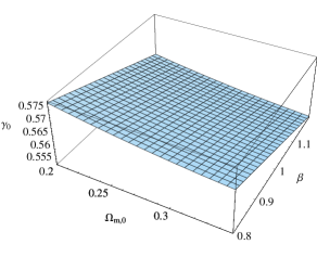
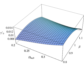
For CDM we have . As was shown in [18], for CDM we have . For , , slightly higher than the constant derived in [31] for a slowly varying DE equation of state and . There is a very slight difference on small resdshifts between the true function and , one could as well use and the agreement would be even better. As the differences are important only on small redshifts. Note also that we find a slightly negative slope so that comes closer to as increases. A definite departure from these values could signal a departure from a CDM universe. More importantly as we will see later a large value for could be a hint for a DE model outside GR. This aspect was already emphasized in [18]. We illustrate in Figure 2 the behaviour of and in function of and inside GR.
As emphasized in [18], equation (36) yields the following identity
| (42) |
whenever to very high accuracy, which is certainly the case in scalar-tensor models as we have seen in Section 2. In other words we have a constraint
| (43) |
As was shown in [18], this constraint takes the following form
| (44) |
The coefficient depends on the background parameters . For given background parameters and , will take the corresponding value . The value of realized will depend on the particular model under consideration and can be obtained numerically. Typically we will have . For models inside General Relativity was obtained. For example for constant , is allmost independent of , with for , while at the same time can have a nonnegligible variation, we have for and .
We can compare scalar-tensor models with different values of but identical background evolution parametrized using the parameters and , according to eqs.(8), (11), (12). These models can be distinguished in all observations affected by a varying gravitational constant but they will be undistinguishable with respect to purely background constraints. In particular, they yield different perturbations growth factor , or equivalently different .
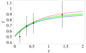
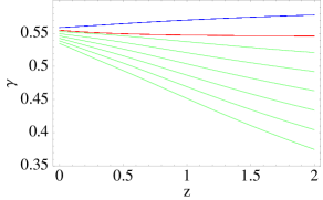
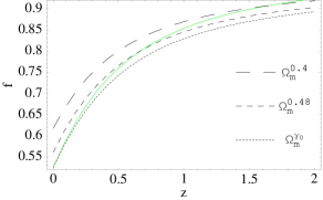
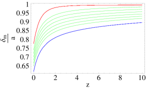
All models shown in Figure 3 have exactly the same background expansion so that the difference in the growth of matter perturbations is solely due to the modification of gravity. As we can see from Figure 3, some models can be easily distinguished from each other using the growth of matter perturbations through the difference in the behaviour of on small redshifts. We note also for the models displayed in Figure 3 that the model inside GR is easily distinguished from the scalar-tensor models having a large slope . For these ST models we have that is negative and it can be large, while it is (slightly) positive for the same background evolution inside GR. Actually as we can see from Figure 2 is true inside GR for the interesting range of cosmological parameters and , while we have generically for the interesting scalar-tensor models. Also, as already noted in [18], inside GR while we see that it can be substantially larger outside GR. Obviously, when is large, assuming constant yields a poor approximation. Another interesting feature is the quasi-linear behaviour of on small redshifts . Such a behaviour could be probed observationnally and could allow to discriminate models whose parameter are close to each other. The lower the value of , the better this potential resolution which improves as well when decreases.
This picture remains essentially the same for the best-fit models of Table 1. It is seen that the growth of matter perturbations on large redshifts is closer to the standard behaviour () in the best-fit scalar-tensor models of Table 1 than it is for the model inside GR with same parametrization of the background expansion. For the latter model, though a very pronounced phantom behaviour is needed today (see Table 1), it is not sufficient to make higher than which has a crucial effect on the growth of matter perturbations on large redshifts.
To summarize, we have shown that our models have a characteristic signature in the growth of linear matter perturbations. On large redshifts inside the matter-dominated stage, we find a scaling behaviour for the matter perturbations which can substantially differ from CDM and also from General Relativity (GR) with identical background evolution characterized, besides , by or . On small redshifts we find again a possible significant departure from CDM and models in General Relativity (GR) with same parametrization of the background expansion. Even for those models in which the growth of matter perturbations on large redshifts is close to that in CDM, we find a large (negative) slope , with much larger than in GR, whether CDM or GR with an identical background evolution. For these models assuming a constant would necessarily lead to a poor fit of the growth function (see Figure 4). Such a behaviour on small redshifts would constitute a characteristic signature of our DE model being outside GR. Interestingly, those models that mimic CDM on large redshifts are most easily distinguished from CDM on small redshifts through their slope . Though the results derived here are to some extent model dependent, it is clear that the growth of matter perturbations, especially when combined on small and large redshifts, can efficiently probe the nature of Dark Energy and in particular help in assessing whether we are dealing with a modified gravity DE model or not.
References
- [1] S.J. Perlmutter et al., Ap. J. 483 565 (1997), Nature 391 51 (1998); A. G. Riess, A. V. Filippenko, P. Challis et al., Astron. J. 116, 1009 (1998); S. J. Perlmutter, G. Aldering, G. Goldhaber et al., Astroph. J. 517, 565 (1999); P. Astier, J. Guy, N. Regnault et al., Astron. Astroph. 447, 31 (2006);
- [2] Adam G. Riess et al., Astrophys. J.659, 98 (2007), e-Print astro-ph/0611572; W. M. Wood-Vasey et al. [ESSENCE Collaboration], Astrophys. J. 666, 694 (2007).
- [3] V. Sahni, A. A. Starobinsky, Int. J. Mod. Phys. D9, 373 (2000); T. Padmanabhan, Phys. Rep. 380, 235 (2003); E. J. Copeland, M. Sami and S. Tsujikawa, hep-th/0603057 (2006); V. Sahni, A. A. Starobinsky, Int. J. Mod. Phys. D15, 2105 (2006); R. Durrer, R. Maartens, Gen. Rel. Grav.40, 301 (2008); P. Ruiz-Lapuente, Class. Quant. Grav.24R91 (2007), e-Print 0704.1058
- [4] W. J. Percival et al. e-Print 0705.3323.
- [5] B. Ratra and P.J.E. Peebles, Phys. Rev. D37 3406 (1988); C. Wetterich, Nucl. Phys. B302 668 (1988).
- [6] T. M. Davis et al., Astrophys. J. 666, 716 (2007).
- [7] N. Bartolo and M. Pietroni, Phys. Rev. D 61 023518 (2000); F. Perrotta, C. Baccigalupi and S. Matarrese, Phys. Rev. D 61, 023507 (2000); Y. Fujii, K. Maeda, The scalar-tensor theory of gravitation, Cambridge Univ. Press (2003); V. Faraoni, Cosmology in Scalar-Tensor Gravity, Kluwer Academic, Dordrecht, 2004.
- [8] B. Boisseau, G. Esposito-Farèse, D. Polarski and A.A. Starobinsky, Phys. Rev. Lett. 85, 2236 (2000).
- [9] G. Esposito-Farèse and D. Polarski, Phys. Rev. D 63, 063504 (2001).
- [10] R. Gannouji, D. Polarski, A. Ranquet, A. A. Starobinsky, JCAP 0609, 016 (2006).
- [11] J. Martin, C. Schimd and J.-P. Uzan, Phys. Rev. Lett.96, 061303 (2006). G. Barenboim, J. Lykken, e-Print 0711.3653; M. Demianski, E. Piedipalumbo, C. Rubano, P. Scudellaro, e-Print 0711.1043; S. Capozziello, P.K.S. Dunsby, E. Piedipalumbo, C. Rubano, e-Print 0706.2615;
- [12] A. A. Starobinsky, JETP Lett. 68, 757 (1998);
- [13] S. Bludman, e-Print astro-ph/0702085; D. Polarski, AIP Conf. Proc. 861, 1013 (2006), e-Print astro-ph/0605532; M. Ishak, A. Upadhye, D. N. Spergel, Phys. Rev. D 74, 043513 (2006).
- [14] L. Knox, Y. S. Song, J. A. Tyson, Phys. Rev. D 74, 023512 (2006); T. Chiba and R. Takahashi, Phys. Rev. D 75, 101301 (2007); P. Zhang, M. Liguori, R. Bean, S. Dodelson, Phys. Rev. Lett.99, 141302 (2007).
- [15] A. F. Heavens, T. D. Kitching, L. Verde, e-Print astro-ph/0703191.
- [16] D. Huterer, E. Linder, astro-ph/0608681; E. Linder, R. Cahn, astro-ph/0701317; S. Tsujikawa, e-Print 0705.1032; C. Di Porto, L. Amendola, e-Print 0707.2686; V. Acquaviva, L. Verde, e-Print 0709.0082; A. Kiakotou, O. Elgaroy, O. Lahav, e-Print 0709.0253; S. Nesseris and L. Perivolaropoulos, Phys. Rev. D 77, 023504 (2008); Y. Wang, e-Print 0710.3885; L. Hui, K. Parfree, e-Print 0712.1162
- [17] Bo Feng, X.-L. Wang, X.-M. Zhang, Phys. Lett.B607, 35 (2005); Hao Wei, Rong-Gen Cai, Ding-Fang Zeng, Class. Quantum Grav.22, 3189 (2005).
- [18] R. Gannouji, D. Polarski, Phys. Lett. B 660, 439 (2008).
- [19] D. Torres, Phys. Rev. D 66, 043522 (2002).
- [20] B. Li, John D. Barrow, Phys.Rev.D 75, 084010 (2007).
- [21] M. Chevallier, D. Polarski, Int. J. Mod. Phys. D10, 213 (2001).
- [22] E. V. Linder, Phys. Rev. Lett. 90, 091301 (2003).
- [23] E. Di Pietro and J. F. Claeskens, Mon. Not. Roy. Astron. Soc. 341, 1299 (2003); S. Nesseris and L. Perivolaropoulos, Phys. Rev. D 70, 043531 (2004); R. Lazkoz, S. Nesseris and L. Perivolaropoulos, JCAP 0511, 010 (2005).
- [24] E. Garcia-Berro, E. Gaztanaga, J. Isern, O. Benvenuto and L. Althaus, e-Print astro-ph/9907440; L. Amendola, P. S. Corasaniti, F. Occhionero, astro-ph/9907222; A. Riazuelo and J. P. Uzan, Phys. Rev. D 66, 023525 (2002);
- [25] D. J. Eisenstein et al. [SDSS Collaboration], Astrophys. J. 633, 560 (2005).
- [26] Y. Wang and P. Mukherjee, Astrophys. J. 650, 1 (2006).
- [27] I. P. Neupane, e-Print: e-Print 0711.3234.
- [28] M. Kunz, D. Sapone, Phys. Rev. Lett. 98, 121301 (2007).
- [29] P. J. E. Peebles, Astrophys. J.284, 439 (1984).
- [30] O. Lahav, P. B. Lilje, J. R. Primack, M. J. Rees, MNRAS251, 128 (1991).
- [31] L. Wang, P. J. Steinhardt, Astrophys. J.508, 483 (1998).
- [32] L. Verde et al., Mon. Not. Roy. Astron. Soc. 335, 432 (2002); E. Hawkins et al., Mon. Not. Roy. Astron. Soc. 346, 78 (2003); M. Tegmark et al. [SDSS Collaboration], Phys. Rev. D 74, 123507 (2006); N. P. Ross et al., arXiv:astro-ph/0612400; J. da Angela et al., arXiv:astro-ph/0612401.