Genus Distributions For Extended Matrix Models Of RNA
Abstract
We construct and study an extended random matrix model of RNA (polymer) folding. A perturbation which acts on all the nucleotides in the chain is added to the action of the RNA partition function. The effect of this perturbation on the partition function and the Genus Distributions is studied. This perturbation distinguishes between the paired and unpaired bases. For example, for (where is the ratio of the strengths of the original and perturbed term in the action) the partition function and genus distribution for odd lengths vanish completely. This partition function and the genus distribution is non-zero for even lengths where structures with fully paired bases only remain. This implies that (i). the genus distributions are different and (ii). there is a “structural transition” (from an “unpaired-paired base phase” to a “completely paired base phase”) as approaches 1 in the extended matrix models. We compare the results of the extended RNA model with the results of G. Vernizzi, H. Orland and A. Zee in PRL 94, 168103(2005).
keywords:
Random Matrix Models, RNA Folding, Perturbation, Genus Distributions, Structural TransitionPACS:
87.14.gn, 87.15.Cc, 11.15.Pg, 11.15.-q, 02.10.Yn1 Introduction
RNA (Ribose Nucleic Acid) is the only known biomolecule which plays the dual role of being a carrier of genetic information and an enzyme in important biological reactions [2]. RNA carries the genetic information from DNA to proteins (where the process of transfer of information from DNA to RNA is referred to as Transcription and from RNA to proteins is called Translation). Over the years, the discovery of enzymatic and other functional roles of ribozymes (larger RNA’s 3000 bases long) have strengthened the importance of RNA in cellular functions. So a study of the RNA structure, classification of different levels of structure, complexity at each level, the energetics and stability have captured the interest of scientists from all genres.
Structurally, bio-polymers have been classified into three
hierarchical levels which are graded in increasing levels of
complexity and instability (in the given order):
(i). Primary Structure : the chemical sequence or the sequence of
nucleotides (planar diagrams), (ii). Secondary Structure : the local
short-range pairing of the complementary Watson-Crick bases A-U and
G-C via hydrogen bonding (planar diagrams) and (iii). Tertiary
structure : the spatial arrangement of secondary units by means of
several van der Waals contacts, hydrogen bonding between the
complementary base pairs and the interactions in which loops and
bulges can themselves partially pair leading to the formation of
pseudoknots (non planar diagrams). Pseudoknots are conformations
whose associated disk diagrams aren’t planar [3] or we can say
that pseudoknots are false knots which have higher genii (a genus
may be understood as the number of handles that a surface has so
that the arcs, representing pairings between the bases, do not
intersect) and are much more complex than the previous two levels of
structures. Most of the work in the field of RNA folding has been
carried out on secondary structures. Monte Carlo techniques and
numerous algorithms are available to solve problems related to
secondary structures [3, 4, 5, 6]. Very little, though is known
about the tertiary structure of RNA because of the complexity
associated with the structures. Immense energies are required to
fold RNA into their folded conformations. The energies involved are
of the order of 100 Kcal/mol or more [7, 8]. In RNA’s, the
complexity increases by manifolds when one goes from secondary to
tertiary structures. Folding of the secondary structures to from
tertiary structures is largely governed by the presence of
ions as demonstrated by experimental studies. The biological
function of RNA is governed by these folded structures i.e the
tertiary structures. So in order to understand the role that RNA’s
play in biological processes it becomes essential to understand
their folded conformations.
Matrix models have proved to be useful and important in areas such as disordered condensed matter systems and quantum chromodynamics among others. These models have been extremely useful in modeling very complex systems. A random matrix model has been proposed in [1, 9] to count and classify all possible structures of RNA which can exist for a given length of the nucleotide chain. However, the number of structures that have been discovered are a very small subset of these vast number of structures. This may be due to the constantly varying conditions inside a living cell. The environment of a cell is subject to changing conditions of temperature, salinity, acidity etc. which act as perturbations to the processes taking place in a cell. These perturbations affect the overall functioning of the cell. So the addition of a perturbation in the potential of the original model of RNA [1, 9] and to observe its effect is very important. In this work a very simple perturbation is studied which does not drastically change the essence of the model proposed in [1, 9]. However, it brings changes in the enumeration of structures of RNA. In particular, for a certain strength of this perturbation a phase of RNA structures with no unpaired bases is found. This will result in a limited activity of the RNA due to the paired conformations alone. Thus a seemingly trivial change in the mathematical structure of the RNA model produces structures of RNA which leads to a non-trivial change in their biological activity.
The random matrix model of RNA folding proposed in [9] is a theoretical model which focuses on the topological aspect of the RNA folding and is constructed as an (NN) matrix field theory. In the model, a matrix is considered which accounts for the attractive energies between the nucleotides, disregards any self interaction of the nucleotides, maintains finite flexibility of the nucleotide chain and the fact that only those nucleotides which are at least 4 nucleotides apart can interact [9]. The model makes use of the notations of quantum chromodynamics in terms of the Feynmann diagrams. In the large N limit, matrix models can be expanded in powers of which also gives a topological expansion as was originally observed by G ’t Hooft [10]. This allows us to identify the tertiary structures as terms with powers of . The RNA matrix model in [1] enumerates all the secondary structures with pseudoknots by making the following simplifications: the polymer chain is assumed to be infinitely flexible so that nucleotides less than 4 nucleotides apart can also interact, sterical constraints are neglected so that any base pairing is allowed irrespective of the type of nucleotide and the interaction between the bases in the chain is assumed to be simple with all the base-pairings taking place with a similar strength ‘v’. This means that the interaction matrix (which is a (LL) matrix, L being the length of the polymer chain) has all the elements equal to ‘v’.
In this paper, section 2 introduces the extended matrix model where a perturbation is added to all the bases in the nucleotide chain keeping the same simplifications as in [1]. A parameter is found which can take different values and hence it distinguishes between the different generalized models. A general form of the partition function for the extended matrix model is found for any length L and . We also discuss the extended matrix model with . In section 3 we discuss the diagrammatic representation of the extended matrix model corresponding to any . Section 4 deals with the genus distributions ( and ) of the extended matrix model, where the odd lengths vanish in the partition function , as approaches 1. We will refer to the RNA folding model in [1, 9] as the RNA-MM and the extended matrix model as RNA-EMM from now on in the literature.
2 Extended Matrix Model of RNA (RNA-EMM) with a Perturbation on all the Bases
We propose an extension of the RNA-MM discussed in [1]. Here we add a perturbation term in the action of the partition function of the nucleotide chain. The partition function of the extended matrix model is,
| (1) | |||||
where are L independent (NN) hermitian matrices, is an (LL) interaction matrix containing interactions between the nucleotides, L being the length of the nucleotide chain, is an ordered product over ’s and is the normalization constant given by,
| (2) |
These RNA matrix models (both RNA-MM and RNA-EMM) are variants of Gaussian Penner Models. Addition of a linear term in this action is non-trivial as shown in references [11, 12] where a linear term is added to the potential of the partition function for the multi-cut matrix model.
The perturbation term in the partition function of equation (1) is,
| (3) |
where , being the strength of the perturbation. We consider . The normalization constant can be written as = where . Carrying out a series of Hubbard Stratonovich Transformations, the integral in equation (1) is reduced to an integral over a single (NN) matrix ,
| (4) |
where . We make a redefinition such that where we define , the ratio of the strength of interaction between the nucleotides to the strength of the perturbation. We therefore get from equation (4),
| (5) |
We now introduce the spectral density of a Gaussian matrix model defined at finite N as,
| (6) |
Making use of the identity in equation (5) the partition function can be written as,
| (7) |
Defining as the exponential generating function of we can write,
| (8) |
| (9) |
where represents Hermite polynomials. Using equation (10) the generating function in equation (9) can be written as,
| (11) | |||||
Rewriting the above equation,
| (12) | |||||
Using a standard result of integration over Hermite polynomials [15],
| (13) |
equation (12) solves to,
| (14) |
| L | ||
|---|---|---|
| 1 | ||
| 2 | v+ | v+ |
| 3 | + | + |
| 4 | ++2+ | ++2+ |
| 5 | +++ | ++5+ |
| 6 | +++ | ++++5+ |
| +5+10 | ||
| 7 | +++ | +++++ |
| ++ | ||
| 8 | +++ | ++++35+ |
| ++ | +14++ | |
| +14+21+70 |
Combining equations (8) and (14) we have,
| (15) |
We observe from equation (15) that by taking different values of (i.e. by varying the ratio of the strengths of interaction between the bases and the perturbation in the action of the partition function) we can have several extensions of the same model. For instance, for , we have the RNA-MM [1]. We substitute in equation (15) and find their corresponding partition functions ( are listed in Table 1). For completeness we write the explicit dependence of the partition function on N in terms of (the topological parameter), genus g, as in [1], . Here, the coefficients ’s give the number of diagrams (structures) at a given length L, genus g and . We also define the total number of diagrams as , for a particular length and , irrespective of the genus.
| L | |
|---|---|
| 1 | 1- |
| 2 | 1+v+-2 |
| 3 | 1+3v-+3-3-3v |
| 4 | 1+6v+2++-4+6+6v-4-12v |
| 5 | 1-+5-10+10-5+10v+10+5-10v+30v- |
| 30v-10-5 | |
| 6 | 1+-6+15-20+15-6+15v+30+15+5+10+15v- |
| 60v+90v+30+15-60v-60-30 | |
| 7 | 1-+7-21+35-35+21-7+21v+70+ |
| 35+35+70-21v+105v-210v-70-35+210v+ | |
| 210+105-105v-210-105-35-70 |
The General Form of : The general form of the partition function for the extended matrix model can be obtained from equation (1) after completing the square in the exponent of the numerator and in the normalization constant in terms of the variable as,
| (16) |
The general form of for the extended matrix model from equation (16) via Wick Theorem is,
| (17) | |||||
We observe that the general form of has the same structure as in [1] with an additional multiplicative factor of powers of on each term (Table 2 lists upto in terms of ’s). The partition functions can be obtained from equation (17) by substituting the desired for a particular length.
| L | ||
| 1 | 1 | 0 |
| 2 | 1+v | v |
| 3 | 1+3v | 0 |
| 4 | 1+6v+2+ | 2+ |
| 5 | 1+10v+10+ | 0 |
| 6 | 1+15v+30+5+ | 5+ |
| 7 | 1+21v+70+35+ | 0 |
| 8 | 1+28v+140+140+14+21+ | 14+70+21 |
| (70+280+70)/ |
Extended Model With : We now substitute in equation (15) i.e. the perturbation is acting on all the bases in the nucleotide chain with a strength the same as the interaction between the bases. We get,
| (18) |
We can see from equation (18) that only even length partition functions will be non-zero whereas for odd lengths, the partition function will vanish (results are summarized in Table 3). It will be shown in the next section that for odd lengths implies that no unpaired base is allowed for the phase. This suggests a considerable change in the genus distributions for the extended matrix model especially for the case when . This is investigated in detail in section 4.
3 Diagrammatic Representation of the Extended Model
We explain in this section the physical interpretation of the general form of obtained in section 2 for the extended matrix model. The general form of the partition function for the extended model is given by equation (17). Each term in the partition function is accompanied by a factor of powers of . The partition function corresponding to (Table 2) is given by or simply . This represents a total of 10 diagrams (Figure 1). In the diagrammatic representation in these models (using quantum chromodynamics), the RNA backbone is represented by a solid line (representing the quark propagator) and the hydrogen bonds between different nucleotides as dotted arcs (representing the gluon propagators) joining two nucleotides on the solid line. Therefore, a primary structure is shown with the nucleotides (or the dots) on the solid line, secondary structure is represented by the arcs (dotted lines) drawn between nucleotides (dots) on the solid line (provided arcs do not intersect) and tertiary structures are those secondary structures in which the arcs intersect [9]. In these diagrams, the powers of ‘v’ give the number of arcs in the corresponding Feynmann diagrams (diagrams are given by the coefficients of the v term). These terms correspond to the planar diagrams. The terms with powers of represent tertiary structures with non-zero genus. The first term in the partition function for is a planar term with each unpaired base associated with the factor of , the second term represents 6 diagrams with one arc each and each unpaired base (2 in number) accompanied by , the third term corresponds to two diagrams with two arcs each and no unpaired bases at all and the last term represents one diagram with two crossing arcs i.e. a tertiary term with genus one and no unpaired bases. These diagrams are shown in Figure 1 with their respective weights. The power of gives the number of unpaired bases in the diagram. However, for the partition function for is given by i.e. a total of 3 diagrams (in Figure 1, the diagrams corresponding to , and ). For this value, only those diagrams with completely paired bases remain. The diagrams with even a single unpaired base are completely suppressed.
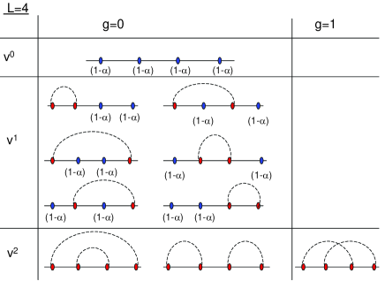
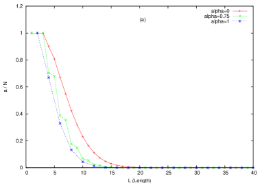
We thus observe that for , all kinds of structures with fully unpaired, partially paired-partially unpaired and completely paired bases exist. However, for , only structures with completely paired bases exist. We refer to these structural differences between the two regions and as a “structural transition” from an “unpaired-paired base phase” to a “completely paired base phase” respectively. Unpaired-paired base phase comprises of all the structures enumerated by the RNA-MM in [1] with different weights associated with each unpaired base for different ’s. A completely paired base phase consists of only those structures which have no unpaired bases at all. For and any given , and , so . This value of the normalized distribution can be seen in Figure 4(a) (i.e. corresponding to ). For and , and , so . This value of the normalized distribution can also be seen in Figure 4(a).
We have seen that this perturbation has created a phase where RNA structures with a limited biological activity (as only structures with paired bases are possible) are separated out from the otherwise possible vast number of structures.
4 Genus Distributions for the Extended Matrix Models
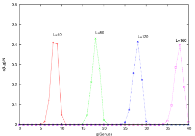
We analyze the genus distributions for the extended matrix model and compare them with the distributions of RNA-MM [1]. We consider in particular the extended matrix model with . For the genus distributions are shown in Figure 2. Figure 2(a) plots the normalized diagrams Vs Length L at a fixed genus g. Figure 2(b) shows a plot of the normalized diagrams Vs g at a particular length L. As indicated by the generating function in equation (18), we find that the partition function for odd lengths vanish (Table 3). The genus distributions are shown in Figure 2.
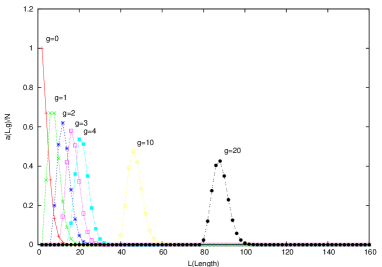
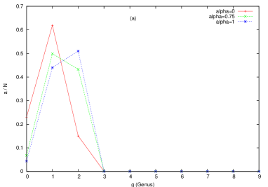
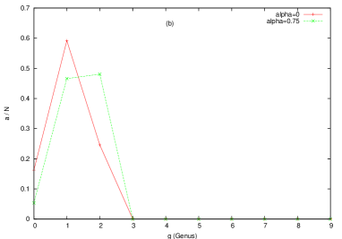
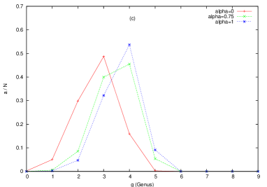
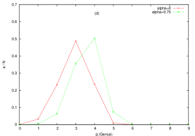
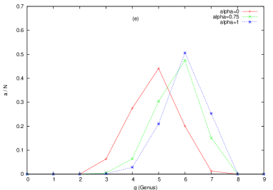
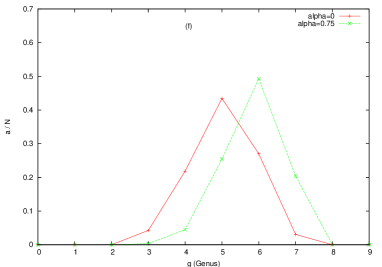
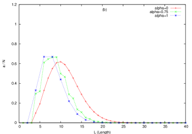
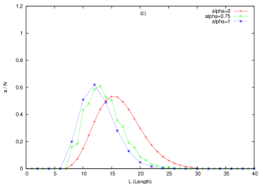
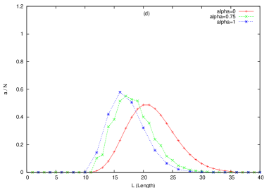
We compare the genus distributions for the following three pairs of successive even and odd lengths: (i). (Figures 3(a), 3(b) respectively), (ii). (Figures 3(c), 3(d) respectively) and (iii). (Figures 3(e), 3(f) respectively), for different values (Figure 3). For a chosen length, plots for different are compared. In the figure with odd length compared to the figure with even length, it is observed that the curve is absent. This is due to the absence of the partition function for odd lengths at . It is also observed that the curve corresponding to at , comprises of points which are an average of the points on the and curves for (same genus points for the two lengths are considered). For example in Figure 3(a) (for ), the points corresponding to for and curves are averaged and the value thus obtained is similar to the value for on the curve in Figure 3(b) (for ). The same is observed on comparison of other lengths ( and ). The shape of the curve for the odd length figure (L=11) seems to take the shape of curve in the even length figure(L=10). This is also observed in the figure Vs L for different genii (g=0,1,2,3) when are plotted together (Figure 4). Notice that in the curve for (Figure 4) for each even-odd length, the points lie close together separated by large distances from the nearest neighboring even-odd lengths.
This analysis extracts the otherwise not so visible differences in the (i). total number of structures and (ii). the shape of genus distributions for different ’s as compared to the distributions in RNA-MM [1]. A study of the genus distributions approaching is particularly important as dramatic changes take place as shown in Figures 3 and 4.
5 Conclusions
We have given a detailed analytic calculation of the partition function after introducing a linear perturbation in the action of the nucleotide chain for the matrix model of RNA folding [1] (section 2). A parameter is found explicitly in the extended matrix model (RNA-EMM). The parameter can be tuned to different values to give several combinations of the strength ratio of the original and the perturbed term thus giving various extensions of the model. For instance, for , the extended matrix model (RNA-EMM) reduces to the RNA-MM in [1]. We find for , the partition function for odd lengths of the polymer chain vanishes completely. This brings significant changes in the genus distributions in terms of the number of structures and the shape of the distribution as compared with the RNA-MM in [1]. We have compared the genus distributions at different lengths and genus for . The curve corresponding to at odd lengths comprises of points which are an average of the points on the and curves on the preceding plot of even length (the same genus for the two lengths is considered for comparison). Also, the shape of the curve for the odd lengths seem to take the shape of curve in the plot of even length (section 4). For other values of we have different results for the partition function (listed in Table 1). The general form of for the extended matrix model consists of an additional multiplicative factor of with each term as compared to [1]. The maximum value of genus g for the extended matrix model for even L and all is found to be i.e. (found numerically). For odd lengths and this result is also true and for there are no diagrams.
The diagrammatic representation of the extended matrix model is discussed in section 3. This follows from the general form of for the extended matrix model found in section 2. The Feynmann diagrams corresponding to length of the polymer chain are shown in Figure 1. Each unpaired base in the polymer chain is associated with a factor of . Hence for odd lengths of the polymer chain when the partition function vanishes. for odd lengths implies that no unpaired base is allowed for the phase. For other values of , the unpaired bases in the chain are weighted by a factor of . We define a “structural transition” where structures change from a “unpaired-paired base phase” to a “completely paired base phase” at (section 4). The perturbation has thus created a phase where RNA structures with a limited biological activity (as only structures with paired bases are possible) are separated out from the otherwise possible vast number of structures (where structures with both paired and unpaired bases are possible).
Our future work will concentrate on a study of more general and realistic perturbations and an analysis of their genus distributions. Another interesting aspect of the problem is to take into consideration Watson-Crick and Wobble (G-U) pairings in the interaction () between the nucleotides so that the condition of a base pairing with any other base (in models discussed so far) is relaxed. This will be a more realistic approach towards the problem of RNA folding but it is not a trivial problem. We would like to study these generalized matrix models with more mathematical rigour as the addition of a linear term in the action can produce non-trivial results as shown in [11, 12] for similar matrix models. The analysis of asymptotics for the extended matrix model (RNA-EMM) will also be dealt with in a future work.
Acknowledgements
In section 3 which discusses the diagrammatic representation for the extended matrix model is inspired by the comments of the referee of Nuclear Physics B. We would like to thank Prof. H. Orland and G. Vernizzi for e-discussions. We would like to thank CSIR Project No. for financial support.
References
- [1] G. Vernizzi, Henri Orland, A. Zee, PRL Vol. 94, 168103 (2005).
- [2] Eric Westhof and Pascal Auffinger, Encyclopedia of Analytical Chemistry R. A. Meyers (Ed.), 5222-5232 (2000).
- [3] M. Pillsbury, H. Orland and A. Zee, Physics Review E, Vol. 72, 011911 (2005).
- [4] M. Pillsbury, J. A. Taylor, H. Orland, and A. Zee, http://arxiv.org/cond-mat/0310505.
- [5] A. P. Gultyaev, Nucleic Acids Res., Vol. 19, 2489 (1991).
- [6] J. P. Abrahams, M. van den Berg, E. van Batenburg and C. W. A. Pleij, Nucleic Acids Res., Vol. 18, 3035 (1990).
- [7] D. H. Turner, N. Sugimoto, S. M. Freier, Annual Review Biophysics Biomolecular Chemistry, Vol. 17, 167 (1988).
- [8] O. C. Uhlenbeck, RNA, Vol. 1, 4 (1995).
- [9] Henri Orland, A. Zee, Nuclear Physics B620[FS], 456 (2002).
- [10] G. ’t Hooft, Nuclear Physics B72, 461 (1974).
- [11] Y. Shimamune, Phys. Letters B108 (1982), 407.
- [12] C. Nappi, Mod. Phys. Letters A5 (1990), 2773.
- [13] See M. L. Mehta, Random Matrices and the Statistical Theory of Energy Levels, 2nd Edn. (Academic, New York, 1991).
- [14] G. Akemann, G. M. Cicuta, L. Molinari, G. Vernizzi, Phys. Rev. E Vol. 59, No. 2, 1489 (1999).
- [15] See I. S. Gradshteyn & I. M. Ryzhik, Table of Integrals, Series & Products, 7th Edn. (Academic, New York, 1965), 837.