Thresholding methods to estimate the copula density
Abstract
This paper deals with the problem of the multivariate copula density estimation. Using wavelet methods we provide two shrinkage procedures based on thresholding rules for which the knowledge of the regularity of the copula density to be estimated is not necessary. These methods, said to be adaptive, are proved to perform very well when adopting the minimax and the maxiset approaches. Moreover we show that these procedures can be discriminated in the maxiset sense. We produce an estimation algorithm whose qualities are evaluated thanks some simulation. Last, we propose a real life application for financial data.
keywords:
copula density, wavelet method, thresholding rules, minimax theory, maxiset theory. AMS Subject Classification: 62G10, 62G20, 62G30.1 Introduction
Recently a new tool has appeared (principally for risk management, for instance in finance, insurance, climatology, hydrology etc) to model the structure of dependance of the data. Let us start by recalling the seminal result of Sklar [17].
Theorem 1 (Sklar (1959))
Let and be a variate distribution function. If, for , any margin of is continuous, there exists a unique variate function with uniform margins such that
The repartition function is called the copula associated to the distribution . The interest of the Sklar Theorem is the following: it is possible to study separately the laws of the coordinates of any vector whose the law is and the dependance between the coordinates.
The Copulas model has been extensively studied in a parametrical framework for the distribution function . Large classes of Copulas, such as the elliptic family, which contains the Gaussian Copulas and the Student Copula, and the archimedian family, which contains the Gumbel Copula, the Clayton Copula and the Frank Copulas, have been identified. Mainly, people have worked in two directions. Firstly, an important activity has concerned the modeling in view to find new Copulas and methodologies to simulate data coming from these new Copulas. Secondly, usual statistical inference (estimation of the parameters, goodness-of-fit test, etc) has been developed using the copulas. As usual, the nonparametric point of view is useful when no a priori model of the phenomenon is specified. For the practitioners, the nonparametrical estimators could be seen as a benchmark allowing to specify the model, comparing with the available parametrical families. This explains the success of the nonparametric estimator of the copula. Unfortunately, the practitioners have difficulties to analyze the graphes concerning the distribution functions (when ). Generally, they try to make comments observing the scatter plot of (or where are the rank statistics of ). Therefore a density estimator could be very advantageous.
We propose procedures to estimate the density associated to the copula . This density denoted is called the copula density. The copula density model that we consider is the following. Let us give a -sample of independent data admitting the same distribution (and the same density ) as . We denote the margins of the coordinates of the vector . We are interested in the estimation of the density copula which is defined as the derivative (if it exists) of the copula distribution
where , and . This model is a very classical density model but the direct observations for of the copula are not available, because the margins are generally unknown. Observe that a similar problem could be the nonparametric regression model with random design. This model has been studied in Kerkyacharian and Picard [15] using warped wavelet families.
In this paper, we focus on wavelet methods. We emphasize that these methods are very well appropriated because the localization properties of the wavelet allow us to give a sharp analysis of the behavior of the copula density near the border of . A great advantage of the wavelet methods in statistics is to provide adaptive procedures in the sense that they automatically adapt to the regularity of the object to be estimated. The problem is a little bit different in the case of the copula. So far, the practitioners use copula densities which are regular. Nevertheless, one of the practical problem is due to the fact that the copula densities are generally concentrated towards the borders of (see Part 6 where simulations are presented). It is very difficult to provide a good estimation when the considered density admits significant jumps (which is the case of the copula density when its support is extended). Observe that the lack of data behind the jumps produce poor estimators and this is just where we are interested by the estimation. The thresholding methods use multifrequency levels depending of the place where the estimator is computed. Consequently, they are really fitted for the problem to estimate the copula density and we think that they outperform the classical linear methods like kernel estimators.
We present in this paper the Local Thresholding Method and the Global (or Block) Thresholding Method. These methods has been first studied by Donoho et al. ([6], [7]) and Kerkyacharian et al. [13]. We prove that the theoretical properties of these procedures with respect to the quadratic risk are as good in the copula density model as in the usual density model (when direct data are available). The good behavior of the usual procedures in the copula density model is also observed when linear procedures are considered (see Genest et al. [9]) and for test problems (see Gayraud and Tribouley [8]). To give an entire overview on the minimax properties of the copula density estimators, we explore the maxiset properties of both procedures (and also of the linear procedure). Again, we prove that the fact that no direct observations are available does not affect the properties of the wavelet procedures: as in the standard density model, the local thresholding method of estimation outperforms the others one.
Next, we provide an important practical study. Another advantage of the wavelet procedures is their remarkable facility of use. Indeed, a large number of implementation of the fast wavelet transform exist and it is just a matter of choice to select one in a given programming language. They can be used almost directly after a simple warping of the original samples. Nevertheless, as noticed previously in the case of the copula density, as most of the pertinent information is located near the border of , the handling of the boundaries should be done with a special care. It is one of the result of the article to show that an inappropriate handling, such as the one proposed by default by a lot of implementation, could cause the wavelet method to fail. The symmetrization/periodization process proposed in this paper is described. To reduce the gridding effect of the wavelet, we further propose to incorporate some limited translation invariance in the method. We first comment our results for simulated data in the case of the usual parametrical copula families and then we present an application on financial data: we propose a method to estimate the copula density imposing that the ”true” copula belongs to a target parametrical family and using the nonparametrical estimator as a benchmark.
The paper is organized as follows. Section deals with the wavelet setting so as to describe the multidimensional wavelet basis used in the sequel. Section aims at describing both thresholding procedures of estimation for which performances shall be studied in Section with the minimax approach and in Section with the maxiset approach. Section is devoted to the practical results. Proofs of main theorems are given in Section and shall need proposition and technical lemmas proved in Appendix.
2 Wavelet setting
Let and be respectively a scaling function and an associated wavelet function. We assume that these functions are compactly supported on for some . See for example the Daubechies’s wavelets (see Daubechies [5]). For any univariate function , we denote by the function where and . In the sequel, we use wavelet expansions for multivariate functions. We build a multivariate wavelet basis as follows:
for all . We keep the same notation for univariate scaling function and multivariate scaling function; the subscripts indicate the number of components. For any the set is an orthonormal basis of and the expansion of any real function of is given by:
where, for any , the wavelet coefficients are
| and |
Roughly speaking, the expansion of the analyzed function on the wavelet basis splits into the ”trend” at the level and the sum of the ”details” for all the larger levels .
3 Estimation procedures
Assuming that the copula density belongs to , we present wavelet procedures of estimation. Motivated by the wavelet expansion, we first estimate the coefficients of the copula density on the wavelet basis. Observe that, for any variate function
which means that the wavelet coefficients of the copula density on the wavelet basis are equal to the coefficients of the joint density on the warped wavelet family
As usual, standard empirical coefficients are
and
| (1) |
Since no direct observation is usually available, we propose to replace this one with the pseudo observation where are the empirical distribution functions associated with the margins. The empirical coefficients are
and
where denotes the rank of for
According to the fact that the wavelet basis is compactly supported, the sum over the indices is finite and is taken over terms. In the sequel, to simplify the notations, we omit the bounds of variation of the indices .
The most natural way to estimate the density is to reconstruct the density thanks to the estimated coefficients. For any indices such that , we consider the very general family of truncated estimators of defined by
| (2) |
where for any . It is intuitive that the more regular is the function , the smallest are the details and then that a good approximation for the function is the trend at a level large enough. Such linear procedures
| (3) |
consisting to put for any have been considered in Genest et al. [9] where a discussion on the choice of is done. It is also possible to consider other truncated procedures as non linear procedures: the local thresholding procedure consists to ”kill” individually the small estimated coefficients considering that they do not give any information. Let be a thresholding level and be the level indices. For and varying between and , the hard local threshold estimators of the wavelet coefficients are
leading to the hard local threshold procedure
| (4) |
It is also possible to decide to ”kill” all the coefficients of the level if the information given by this level is too small. For a thresholding level and for levels varying between and , we define the hard global threshold estimates of the wavelet coefficients as follows
leading to the hard global threshold procedure
| (5) |
The non linear procedures given in (4) and (5) depend on the levels indices and on the thresholding level to be chosen by the user. In the next part, we explain how to determine these parameters such a way that the associated procedures achieve optimality properties. We need then to define a criterion to measure the performance of our procedure.
4 Minimax Results
4.1 Minimax approach
A well-known way to analyze the performances of procedures of estimation is the minimax theory which has been extensively developed since the 1980-ies. In the minimax setting, the practitioner chooses a loss function to measure the loss due to the studied procedure and a functional space where the unknown object to estimated is supposed to belong. The choice of this space is important because the first step (when the minimax theory is applied) consists to compute the minimax risk associated to this functional space. This quantity
(where the infimum is taken over all the estimators of ) is a lower bound giving the best rate achievable on the space . When a statistician proposes an estimation procedure for functions belonging to , he has to evaluate the risk of his procedure and compare this upper bound with the minimax risk. If the rates coincide, the procedure is minimax optimal on the space . A lot of minimax results for many statistical models and many families of functional spaces as Sobolev spaces, Holder spaces, and others as the family of Besov spaces have been now established (see for instance Ibragimov and Khasminski [11] or Kerkyacharian and Picard [12]).
4.2 Besov spaces
Since we deal with wavelet methods, it is very natural to consider Besov spaces as functional spaces because they are characterized in term of wavelet coefficients as follows
Definition 1 (Strong Besov spaces)
For any , a function belongs to the Besov space if and only if its sequence of wavelet coefficients satisfies
An advantage of the Besov spaces is to provide a useful tool to classify wavelet decomposed signals according to their regularity and sparsity properties (see for instance Donoho and Johnstone [6]). Last, it is well known that the minimax risk measured with the quadratic loss on this space is
where the infimum is taken other any estimator of the density .
4.3 Optimality
Let us focus on the quadratic loss function. Choosing a wavelet regular enough and when , Genest et al. [9] prove that the linear procedure defined in (3) provides an optimal estimator on the Besov space for some fixed as soon as is chosen as follows:
On a practical point of view, this result is not completely satisfying because the optimal procedure depends on the regularity of the density which is generally unknown. To avoid this drawback, many works in the nonparametric setting as in Cohen et al. [12], in Kerkyacharian and Picard [14] inspired from Donoho and Johnstone’s studies on shrinkage procedures (see for instance [6]) build adaptive procedures which means that they do not depend on some a priori information about the unknown density. For instance, note that the thresholding procedures described in (4) and (5) are clearly adaptive. The following theorem (which proof is a direct consequence of Theorem 4 established in the next section by considering some inclusion spaces properties) gives results on their rates
Theorem 2
Let us consider a continuously differentiable wavelet function and let . Let us choose the integers and and the real such that
for some . Let be either the hard local thresholding procedure or the hard global thresholding procedure . Then, as soon as is large enough, we get
We immediately deduce
Corollary 4.1
The hard local thresholding procedure and the hard global thresholding procedure are adaptive near optimal up to a logarithmic term (that is the price to pay for adaptation) on the Besov spaces for the quadratic loss function, according to the minimax point of view.
Observe that if then the assumption in Theorem 2 could be replaced by because in this particular case .
4.4 Criticism on the minimax point of view
On a practical point of view, the first drawback of the minimax theory is the necessity to fix a functional space. Corollary 4.1 establishes that no procedure could be better on the space than our hard thresholding procedures (up to the logarithm factor) but this space is generally an abstraction for the practitioner. Moreover, this one knows that his optimal procedure achieves the best rate but he does not know this rate. An answer to this drawback is given by Lepski by introducing the concept of the random normalized factor (see Hoffmann and Lepski [10]).
Secondly, he has the choice between both procedures since Theorem 2 establishes that the hard thresholding procedures (local and global) have the same performances when dealing with the minimax point of view. Nevertheless, a natural question arises here: is it possible to compare thresholding procedures for estimation of the copula density between themselves? To answer to these remarks, we propose to explore in the next part the maxiset approach.
5 Maxiset Results
5.1 Maxiset approach
The maxiset point of view has been developed by Cohen et al. [4] and is inspired from recent studies in the approximation theory field. This approach aims at providing a new way to analyze the performances of the estimation procedures. Contrary to the minimax setting, the maxiset approach consists in finding the maximal space of functions (called the maxiset) for which a given procedure attains a prescribed rate of convergence. According to this, the maxiset setting is not so far from the minimax one. Nevertheless it seems to be more optimistic than the minimax point of view in the sense that the maxiset approach points out all the functions well-estimated by a fixed procedure at a given accuracy.
In the sequel, we say that a functional space, namely , is the maxiset of a fixed estimation procedure associated with the rate of convergence if and only if the following equivalence is satisfied
Notice that the considered loss function is again the quadratic one. As a first consequence of adopting the maxiset point of view, we observe that if is an estimator of achieving the minimax rate of convergence on a functional space then is included in the maxiset of associated with the rate but is not necessarily the same. Therefore, it could be possible to distinguish between both optimal minimax procedures: for the same target rate, the best procedure is the procedure admitting the largest maxiset.
Recently many papers based on the maxiset approach have arisen when considering the white noise model. For instance it has been proved in Autin et al. [2] that the hard local thresholding procedure is the best one, in the maxiset sense, among a large family of shrinkage procedures, called the elitist rules, composed of all the wavelet procedures only using in their construction empirical wavelet coefficients with absolute value larger than a prescribed quantity. This optimality has been already pointed out by Autin [1] in density estimation who has proved that weak Besov spaces are the saturation spaces of elitist procedures.
5.2 Weak Besov spaces
To model the sparsity property of functions, a very convenient and natural tool consists in introducing the following particular class of Lorentz spaces, namely weak Besov spaces, that are in addition directly connected to the estimation procedures considered in this paper. We give definitions of the weak Besov spaces depending on the wavelet basis. However, as is established in Meyer [16] and Cohen et al. [4], most of them have also different definitions proving that this dependence in the basis is not crucial at all.
Definition 2 (Local weak Besov spaces)
For any , a function belongs to the local weak Besov space if and only if its sequence of wavelet coefficients satisfies the following equivalent properties:
-
•
-
•
Definition 3 (Global weak Besov spaces)
For any , a function belongs to the global weak Besov space if and only if its sequence of wavelet coefficients satisfies the following equivalent properties:
-
•
-
•
The equivalences between the properties used in the definition of global weak Besov spaces and in the definition of local weak Besov spaces can be proved using same technics as those proposed in Cohen et al. [4].
We prove in Section 7.3 the following link between the global weak Besov space and the local weak Besov space
Proposition 1
For any , we get .
Last, we give an upper bound for the estimation expected error (when the thresholding procedures are used) in the standard density model (i.e. when direct observations are available). Notice that this result is stronger than the result given in the minimax part because the functional assumption is weaker.
Theorem 3
Let be either or and be the estimator built in the same way as but with the sequence of coefficients defined in (1). Let and assume that
Then, there exists some such that for any
5.3 Performances and comparison of our procedures
In this section, we study the maxiset performances of the linear procedure and of the thresholding procedures described in Section . We focus on the optimal minimax procedures which means that we consider the following choices of parameters:
Let us fix . we choose to focus on the (near) minimax rate achieved on the space . The following theorem exhibits the maxisets of the three procedures associated with the same target rate .
Theorem 4
Let and assume that . For a large choice of , we have
| (8) | |||||
It is important to notice that, according to Theorem 3, the fact that direct observations are not available does not affect the maxiset performances of our procedures. As remarked by Autin et al. [3] we have clearly
We deduce by using Proposition 1 that both thresholding estimators considered in Theorem 2 achieve the minimax rate (up to the logarithmic term) on a larger functional space than which is the required space in the minimax approach. In particular, Theorem 2 is proved. We propose now to discriminate these procedures by comparing their maxisets. Thanks to Theorem 4 and applying the inclusion property given in Proposition 1, we prove in Section 7.3 the following corollary
Corollary 5.1
Let and let us consider the target rate
We get
Hence, in the maxiset point of view and when the quadratic loss is considered, the thresholding rules outperform the linear procedure. Moreover, the hard local thresholding estimator appears to be the best estimator among the considered procedures since it strictly outperforms the hard global thresholding estimator .
6 Applied results
This part is not only an illustration of the theoretical part. First, we explain the considered algorithm with several numerical possibilities to overcome any drawback. Next, we test the qualities of our methodology with some simulation and we define the best choices among our propositions. Last, we apply the chosen procedure for financial data.
6.1 Algorithms
The estimation algorithms are described here for for sake of simplicity but their extension in any other dimension is straightforward. We therefore assume that a sequence of samples is given.
All estimators proposed in this paper can be summarized in a 7 steps algorithm:
-
1.
Rank the with
-
2.
Compute the maximal scale index .
-
3.
Compute the empirical scaling coefficients at the maximal scale index :
-
4.
Compute the empirical wavelet coefficients from this scaling coefficients with the fast 2D wavelet transform algorithm.
-
5.
Threshold these coefficients according to the global thresholding rule or the local thresholding rule to obtained the estimated wavelet coefficients or .
-
6.
Compute the estimated scaling coefficients at scale index by the fast 2D wavelet inverse transform algorithm.
-
7.
Construct the estimated copula density by the formula
Unfortunately only the steps , and are as straightforward as they seem. In all the other steps, one has to tackle with two issues: the handling of the boundaries and the fact that the results are not a function but a finite matrix of values.
The later issue is probably the easiest to solve. It means that we should fix a number of point larger than and approximate the estimated copula density at step on the induced grid . We can not compute exactly the value on the grid as the scaling function is not always known explicitly. Nevertheless a very good approximation can be computed on this grid and we neglect the effect of this approximation. From the numerical point of view, this implies that the estimation error can be computed only on this grid and thus that the norms appearing in the numerical results (see Table 1, Table 2, Table 4 and Table 3) are empirical norms on this grid. In this paper, we choose . Note that step also require an evaluation of the scaling function and thus is replaced by an approximation.
The former issue, the boundaries effect, is the key issue here. Indeed, for most copula densities, the interesting behavior arises in the corners which are the most difficult part to handle numerically. The classical construction of the wavelet yields a basis over while we only have samples on .
-
•
A first choice is to consider the function of to be estimated as a function of which is null outside . This choice is called zero padding as it impose the value outside .
-
•
A second choice is to suppose that we observe the restriction on of a -periodic function, this is equivalent to work in the classical periodic wavelet setting. This choice called periodization is very efficient if the function is really periodic.
-
•
We propose also to modify the periodization and assume that we observe the restriction over of a even -periodic function. As we introduce a symmetrization over the existing borders, we call this method symmetrization. It avoids the introduction of discontinuities along the border. Note that nevertheless this symmetrization introduces a discontinuities in the derivatives on the boundaries.
Once this extension has been performed on the sample, one can apply the classical wavelet transform. The resulting estimated copula density is the restriction to of the estimated function.
The wavelet thresholding methods in a basis suffer from a gridding effect: we can often recognize a single wavelet in the estimated signal. To overcome this effect, we propose to use the cycle spinning trick proposed by Donoho and Johnstone. To add some translation invariance to the estimation process, we estimate the copula density with a collection of basis obtained by a simple translation from a single one and to average the resulting estimate. In our numerical experiments, we have performed this operation with different translation parameters and observed that it has always ameliorate our estimate.
6.2 Simulation
We focus on the usual parametrical families of copulas: the FGM, the Gaussian, the Student, the Clayton, the Frank and the Gumbel families. We give results for both values of (the number of data): is very small for bidimensional problems and is usual in nonparametric estimation.
We test both methods of estimation and three ways to solve the boundaries problems. We simulated data with the same copula, the first margin being exponential with parameter and the second margin being standard gaussian. Obviously, because of our algorithm, the results are exactly the same when we change the laws of the margins.
To evaluate the quality of our results, we consider three empirical loss functions deriving from the norm, norm and norm:
where is the ”true” copula density and is the number of points of the grid (see the previous part). Table 4 and Table 3 summarize the estimation relative errors
These relative errors are computed with repetitions of the experiment. The associated standard deviation is also given (in parentheses).
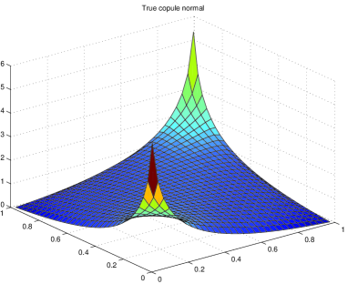
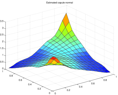
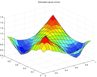
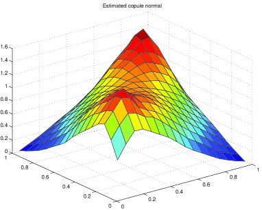
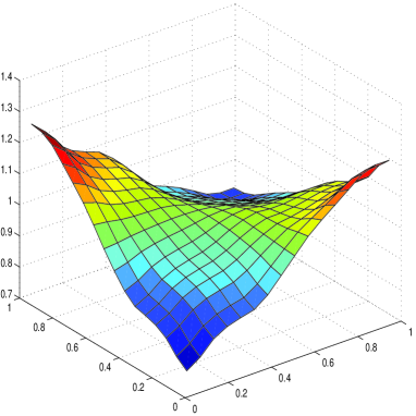
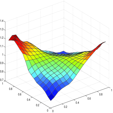
Table 1 and Table 2 show that the zero-padding method and the periodization method give similar results and lead to errors which are generally much larger than the symmetric periodization which is the best method to solve the boundaries effects. This remark is valid for . Although the zero-padding method is the default method with the Matlab Wavelet Toolbox, it suffers from a severe drawback: it introduces a strong discontinuities along the borders of . The periodization method suffers from the same drawback than the zero-padding method as soon as the function is not really periodic. Figure 1 emphasizes the superiority of the symmetric periodization method in the case where the unknown copula density is a normal copula. While the copula estimated with symmetric extension remains close from the shape of the true copula except for the resolution issue, this is not the case for the two other estimated copulas: in the periodized version, the height of the extreme peaks is reduced and two spurious peaks corresponding to the periodization of the real peaks appear. The zero padded version shows here only the reduced height artifact.
Tables 3 and 4 display the empirical , and estimation error for the symmetric extension for respectively and . Globally, they show that the best results are obtained for the norm for which the method has been designed. The second best results are obtained for the norm because a bound on the norm implies a bound on the norm. The estimation in is much harder as it is not a consequence of the estimation in and can be considered as a challenge for such a method.
One can also observed that the behavior largely depends on the copula itself. This is coherent with the theory that states that the more “regular” the copula is the more efficient the estimator will be. The copulas that are the least well estimated (Normal with parameter .9, Student with parameter .5 and Gumbel with parameter 8.33) are the most “irregular” ones. They are very “peaky” for the last two and almost singular along the first axis for the first one. They are therefore not enough regular to be estimated correctly by the proposed method.
A final remark should be given on the difficulty to evaluate such these errors. Whereas the norm is finite equal to for all true copula, the and norm can be very large even infinite because of their peaks. This is not an issue from the numerical point of view as we are restricted to a grid of step on which one can ensure the finiteness of the copula. Nevertheless the induce “empirical” norm can be substantially different from the integrated norm. Thus the error for to are not strictly equivalent as the function can be much more complex for the resolution induced by than for .
6.3 Real data applications
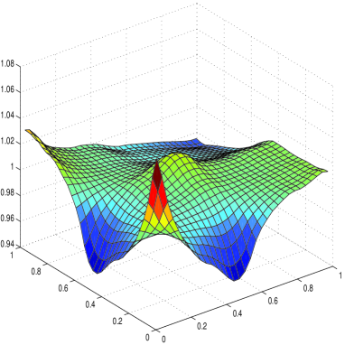
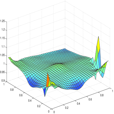
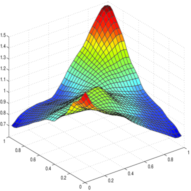
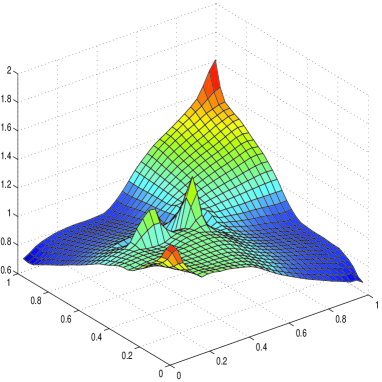
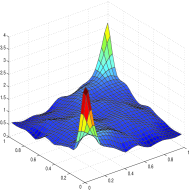
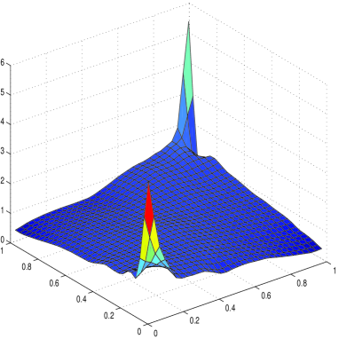
We apply the thresholding methods on various financial series to identify the behavior of the dependance (or non dependance). All our data correspond to daily closing market quotations and are from 01/07/1987 to 31/01/2007. As usual, we consider the return of the data. Note that the data of each samples are not necessary independent but we apply our procedures as there were. We first propose estimators of the bivariate copula density associated with two financial series using the adaptive thresholding procedures (see Figure 2– Figure 5). Next, the nonparametrical estimator denoted is used as a benchmark and we derive an new estimator by minimization of the error between the benchmark and a given parametrical family of copula densities. As previously, we focus on copulas which belong on the Gaussian, Student, Gumbel, Clayton or Frank families. More precisely, we consider the following parametric classes of copulas
We consider three distances
where . We propose to estimate the parameter for each class of copula densities as follows
which appears to be the best estimator of under the constraint that the copula belongs to a fixed parametrical family. We derive estimators of among all the candidates for each contrast . Table 5– Table 8 give
-
•
the parameter for defined by
-
•
the parametric family corresponding to the smallest error ,
-
•
the associated relative errors defined by
where is in .
We test a lot of financial series and we select four revealing examples: we never observe that the Clayton family or the Gumbel family contains the best choice to model the unknown copula; the families used are always the Student class or the Frank class.
First, we observe that the results are very good since any computed relative error is small (in the worst case ). The results are quite similar for both thresholding methods when the unknown copula density does not present high picks (but the last one: DowJones versus Ftse100uk). In a theoretical point of view, we prefer the block thresholding method because the estimator are smoother. See by instance the case of the copula between Brent and ExonMobil where the picks appearing in Figure 3 (on the right) are not pleasant (even if their ranges are not so large). Moreover, the relative error computed with the parametrical density which is the best one among all the possible parametrical copula densities is generally smallest for the block thresholding method.
Notice that the choice of the contrast is crucial to estimate the parameter : there are significative differences between . This is usual in density estimation. We prefer to measure the loss due to the estimator with the norm because this norm is very adapted to the human eye and then the graphical results are the best. The quadratic loss is frequently used because the graphical results are easier to obtain but our opinion is that this norm does not emphasize enough differences between the densities. See by instance the very small relative errors computed with the contrast. The norm has the opposite behavior: it accentuates every difference. It could be a drawback when the local thresholding method is considered and when to many details are kept (see again the case of the copula of the couple Brent/ExonMobil).
Nevertheless, the choice of the best family do not depend on the choice of the contrast: it is fundamental because each type of parametrical family is linked to a specific behavior of the dependance and then the practitioner asks for indications about the copula type. The study of the copula Cac versus Brent allows to decide that both series are independent. Observe that there are small problems on the borders (but notice the very small scaling) although our methodology is made to remove this artefact. We think that a usual linear kernel method becomes disastrous when the copula density comes near of the uniform. The copula densities DowJones versus Oncedor and Brent versus ExonMobil are both Frank copulas but with opposite behaviors. It seems natural that the series Brent and ExonMobil are dependent and varying in the same sense. Oncedor (gold) is an hedge when the stock market collapses which could explain the negative dependance between Oncedor and the financial indices (we observe the same kind of dependance for others indices like Fste100uk, Cac …). The more delicate case is for the copula DowJones versus Fste100uk because the picks are more accentuated. In this case, the local thresholding method produces a nice Figure.
In conclusion, we present here an estimation method which is popular among the practitioners: first, the nonparametrical estimator could be see as a benchmark to decide graphically if the unknown copula density looks like a copula density belonging to a well known parametrical family. In this case, the parameter is estimated with plug-in methods using the benchmark. We do not study here the properties of such an estimator or the goodness-of-fit test problem. For a statistic test procedure, we refer to Gayraud and Tribouley (2008).
7 Proofs
We first state the propositions needed to establish the main results. Next, we prove Theorem 4 in two steps by proving both implications. Last, we establish Proposition 1 and Corollary 5.1.
From now on we denote any constant that may change from one line to another, which does not depend on , and but which depends on the wavelet and on and .
7.1 Preliminaries
These preliminary results concern the estimation of the wavelet coefficients and the scaling coefficients (denoted with to unify the notation). Proposition 3 announces that the accuracy of the estimation is as sharp as if the direct observations were available.
Proposition 2
Assume that the copula density belongs to and let . There exists a constant such that for any such that , and for any
| (9) | |||||
| (10) |
as soon as is chosen large enough.
It is clear that (10) is a direct consequence of (9). Proof of (9) is rejected to the Appendix. Note that from (9) we immediately deduce
Proposition 3
Under the same assumptions as in Proposition 2 on and , there exists a constant such that for any
7.2 Proof of Theorem 4
First, we prove the result for the linear estimator. Secondly, we prove the result for the local thresholding method. We do not prove the result for the global thresholding method since the technics are the same except that the required large deviation inequality established in Proposition 2 is given by (10) instead of (9).
7.2.1 Proof of Equivalence (8)
On the one hand, let be a copula density function belonging to satisfying for any ,
| (11) |
for some constant . Let us prove that also belongs to the space . Let us recall that the smoothing index used for the linear procedure is satisfying . Since
and following the assumption (11), we get
which is the announced result. On the other hand, let us suppose that . Then, using the same technics as in Genest et al. [9], we prove that
which ends the proof. The proof in Genest et al. [9] is given in the case and need some sharp control on the estimated coefficients because an optimal result is established (there is no logarithmic term in the rate).
7.2.2 Proof of Equivalence (first step: )
When direct observations are available, we use the estimator built in the same way as but with the sequence of coefficients defined in (1) and the threshold instead of . Let us take positive integers and . Since we get
we have then to study the error term due to the fact that we use pseudo observations
Using Proposition 3, we have
| (12) |
For the study of , we separate the cases where the wavelet coefficients are larger or smaller than the thresholding level . By Cauchy-Schwartz Inequality, we have
Observe that, for any , we have
| (13) |
For any , we use now the standard Bernstein Inequality to obtain
| (14) |
which is valid for a choice of large enough. Let us now fix in . Applying Proposition 3 and using (13), it follows
for
Similarly, we have
for
implying that
Using (13) and Proposition 2, we get
Combining the bounds of and choosing as indicated in Theorem 2, we get for
where
On the one hand, let us suppose that belongs to the weak Besov which means that (for )
It follows that
Using the standard result given in Theorem 3 when direct observations are available, we also have
as soon as . This ends the proof of the first part of (8) of Theorem 4.
7.2.3 Proof of Equivalence (second step: )
Suppose that there exists such that for any , Since
and choosing as indicated in Theorem 2, we obtain
Using Definition 1 of the strong Besov spaces, we deduce that belongs necessarily to . Let us now study the sum of the square of the details when the details coefficients are small
Since we have already proved that and taking as indicated in Theorem 2, we deduce
Taking as in Theorem 2, we get
Observe that
Remembering that
and using Proposition 2 and (14), we get
as soon as is larger than . Combining using Definition 2 of the local weak Besov space, we conclude that with such that . Hence, we end the proof of the indirect direction of (8).
7.3 Proofs of Proposition 1 and Corollary 5.1
The proof of the large inclusion given in Proposition 1 follows immediately from the definitions of the functional spaces. Denote the sequence of wavelet coefficients of a function . Since we have
it follows from Definition 3 that
To establish the strict inclusions, we build a sparse function belonging to but not to . Let us choose a real number such that . Let us consider a function with the sparse sequence such that at each level and at each , only wavelet coefficients take the value . The others are equal to . For all let be such that . We get
implying that
and the function belongs to the local weak Besov space Next, put and observe that since . For all let be such that . We get
implying
It follows that the function does not belong to the global weak Besov which ends the proof of Proposition 1. Notice that the function belongs to the strong Besov space because for all
implying that
Corollary 5.1 is also proved too.
8 Appendix
This section aims at proving (9) of Proposition 2. In the sequel we fix the indices and and take without loss of generality . For any (the observation index) and any (the coordinate index), let us introduce the following notations
as univariate quantities and
as variate quantities. As previously remarked in Genest et al. [9] (for ), from the definitions above we have
| (15) | |||||
In the sequel, for , we denote by any term of the type
i.e. such that there are exactly factors appearing in the product. The cardinality of such terms is equal to . Observe that the number of terms in (15) is . It is fundamental to notice that there is no term .
8.1 Technical lemmas
We begin by giving technical lemmas.
Lemma 1
There exists a universal constant such that for any
Lemma 1 is a consequence of the Dvoreski-Kiefer-Wolfovitz inequality. For the interested reader, the detailed proof of this lemma is given in Autin et al. [3].
Lemma 2
Let and be an integer such that . Then, there exists such that for any level satisfying
and for any ,
Lemma 3
Let us assume that belongs to and let . For all , for all subsets and of with cardinalities equal to and having no common component, let us put for ,
| (16) |
with the following notation .
For any ,
we have
where are constants such that
Lemma 3 is a direct application of the Bernstein Inequality with
and in the same way,
and
8.2 Proof of Proposition 2
By Equality (15), we have for any
for
Using a Taylor expansion, the following inequality holds for and
implying that, for an associated
For , let us introduce the following events
| , | ||||
| , |
It follows that for any and any
where
Fix and take . Using Lemma 1 and Lemma 2, one gets
| (17) |
as soon as . Since , we apply Lemma 3 and we obtain
as soon as
| (18) |
Let us restrict ourselves to the case where:
Assuming that is large enough and that is chosen large enough, Condition (18) on is satisfied if, for any
This condition is always satisfied since . We obtain the announced result.
References
- [1] Autin, F. (2006) Maxisets for density estimation on . (2006). Math. Methods of Statist., n 2, 123-145.
- [2] Autin, F., Picard, D. and Rivoirard, V. (2006). Maxiset approach for Bayesian nonparametric estimation. Math. Methods of Statist., vol 15, n 4, 349-373.
- [3] Autin, F., Le Pennec, E. and Tribouley, K. (2008). Thresholding methods to estimate the copula density. preprint on the web (http://www.cmi.univ-mrs.fr/ autin/DONNEES/COPULAS).
- [4] Cohen, A., De Vore, R., Kerkyacharian, G. and Picard, D. (2001). Maximal spaces with given rate of convergence for thresholding algorithms. Appl. Comput. Harmon. Anal., 11, 167-191.
- [5] Daubechies, I. (1992). Ten Lectures on Wavelets. SIAM, Philadelphia.
- [6] Donoho, D.L., Johnstone, I. (1995). Adapting to unknown smoothness via wavelet shrinkage. J. Am. Stat. Assoc, 90(432), 1200-1224.
- [7] Donoho, D.L., Johnstone, I.M., Kerkyacharian, G. and Picard, D.(1996). Density estimation by wavelet thresholding. Annals of Statistics, 24, 508-539.
- [8] Gayraud, G., and Tribouley, K. (2008). Good-fit-of test for the copula density. Submitted paper.
- [9] Genest, C., Masiello, E. and Tribouley, K. (2008). Estimating copula densities through wavelets. Submitted paper.
- [10] Hoffmann, M. and Lepski, O. V. (2002). Random rates in anisotropic regression. With discussions and a rejoinder by the authors. Ann. Statist., 30,(2), 325-396.
- [11] Ibragimov, I. A. and Khasminski, R. Z. (1981). Statistical estimation. Springer-Verlag, New-York. Asymptotic theory, translated from the Russian by Samuel Kotz.
- [12] Kerkyacharian, G., Picard, D. (1992). Density estimation in Besov spaces. Statistics and Probability Letters, 13, 15-24.
- [13] Kerkyacharian, G., Picard, D., Tribouley, K. (1996). adaptive desnity estimation. Bernoulli, 2 229-247.
- [14] Kerkyacharian, G., Picard, D. (2001). Thresholding algorithms, maxisets and well concentrated bases. Test, 9 n 2, 283-344.
- [15] Kerkyacharian, G., Picard, D. (2004). Regression in random design and warped wavelets. Bernoulli,10 1053-1105.
- [16] Meyer, Y. (1990). Ondelettes et Opérateurs, Hermann, Paris.
- [17] Sklar, A. (1959). Fonctions de répartition à dimensions et leurs marges. Publ. Inst. Statist. Univ. Paris, 8, 229-231.
Correspondances:
AUTIN Florent, LATP, université Aix-Marseille 1, Centre de Mathématiques et Informatique, 39 rue F. Joliot Curie, 13453 Marseille Cedex 13 (autin@cmi.univ-mrs.fr).
LEPENNEC Erwan, LPMA, université Paris 7, 175 rue du Chevaleret, 75013 Paris (lepennec@math.jussieu.fr).
TRIBOULEY Karine, LPMA, 175 rue du Chevaleret, 75013 Paris and MODALX, Université Paris 10-Nanterre, 200 avenue de la République, 92001 Nanterre Cedex (ktriboul@u-paris10.fr ).
 |
 |
|
| (a) | (b) | |
 |
 |
|
| (c) | (d) |
| Copula | Method | Boundaries Handling | |||
| par. | sym | per | ZeroPad | ||
| FGM | 1.0 | Local | 0.007 (0.003) | 0.079 (0.005) | 0.129 (0.010) |
| Block | 0.006 (0.002) | 0.077 (0.008) | 0.141 (0.006) | ||
| normal | 0.0 | Local | 0.002 (0.002) | 0.0004 (0.0004) | 0.122 (0.005) |
| Block | 0.002 (0.002) | 0.0004 (0.0006) | 0.105 (0.001) | ||
| normal | Local | 0.031 (0.007) | 0.161 (0.011) | 0.179 (0.010) | |
| Block | 0.032 (0.008) | 0.154 (0.011) | 0.202 (0.005) | ||
| normal | 0.9 | Local | 0.156 (0.011) | 0.391 (0.008) | 0.418 (0.006) |
| Block | 0.140 (0.009) | 0.381 (0.005) | 0.491 (0.022) | ||
| Student | (0.5,1) | Local | 0.326 (0.018) | 0.460 (0.008) | 0.544 (0.009) |
| Block | 0.324 (0.026) | 0.458 (0.010) | 0.585 (0.004) | ||
| Clayton | Local | 0.075 (0.013) | 0.225 (0.010) | 0.252 (0.011) | |
| Block | 0.095 (0.012) | 0.216 (0.011) | 0.279 (0.005) | ||
| Frank | Local | 0.021 (0.006) | 0.149 (0.015) | 0.212 (0.015) | |
| Block | 0.013 (0.006) | 0.134 (0.009) | 0.193 (0.006) | ||
| Gumbel | 8.3 | Local | 0.701 (0.002) | 0.849 (0.001) | 0.866 (0.001) |
| Block | 0.698 (0.002) | 0.852 (0.001) | 0.878 (0.001) | ||
| Gumbel | Local | 0.038 (0.010) | 0.104 (0.005) | 0.172 (0.009) | |
| Block | 0.052 (0.007) | 0.109 (0.004) | 0.173 (0.004) | ||
| Copula | Method | Boundaries Handling | |||
| par. | sym | per | ZeroPad | ||
| FGM | 1.0 | Local | 0.0036 (0.0012) | 0.0659 (0.0044) | 0.0897 (0.0037) |
| Block | 0.0037 (0.0015) | 0.0599 (0.0029) | 0.1068 (0.0041) | ||
| normal | 0.0 | Local | 0.0006 (0.0005) | 0.0001 (0.0001) | 0.0828 (0.0019) |
| Block | 0.0006 (0.0007) | 0.0001 (0.0001) | 0.0916 (0.0020) | ||
| normal | Local | 0.0176 (0.0032) | 0.1449 (0.0040) | 0.1421 (0.0046) | |
| Block | 0.0177 (0.0029) | 0.1329 (0.0036) | 0.1518 (0.0055) | ||
| normal | 0.9 | Local | 0.1376 (0.0052) | 0.3893 (0.0031) | 0.4024 (0.0033) |
| Block | 0.1330 (0.0045) | 0.3813 (0.0027) | 0.4261 (0.0046) | ||
| Student | (0.5,1) | Local | 0.2966 (0.0056) | 0.4519 (0.0037) | 0.5197 (0.0036) |
| Block | 0.2881 (0.0058) | 0.4467 (0.0029) | 0.5230 (0.0028) | ||
| Clayton | Local | 0.0603 (0.0053) | 0.2073 (0.0046) | 0.2127 (0.0041) | |
| Block | 0.0596 (0.0054) | 0.1968 (0.0030) | 0.2247 (0.0071) | ||
| Frank | Local | 0.01208 (0.0032) | 0.1244 (0.0047) | 0.1186 (0.0043) | |
| Block | 0.0075 (0.0017) | 0.1137 (0.0035) | 0.1218 (0.0048) | ||
| Gumbel | 8.3 | Local | 0.6975 (0.0015) | 0.8511 (0.0004) | 0.8664 (0.0003) |
| Block | 0.6971 (0.0012) | 0.8520 (0.0004) | 0.8642 (0.0003) | ||
| Gumbel | Local | 0.0240 (0.0041) | 0.1022 (0.0030) | 0.1392 (0.0029) | |
| Block | 0.0336 (0.0042) | 0.0988 (0.0026) | 0.1503 (0.0038) | ||
| Copula | Method | Empirical Loss Function | |||
| par. | |||||
| FGM | 1.0 | Local | 0.062 (0.014) | 0.007 (0.003) | 0.189 (0.051) |
| Block | 0.061 (0.011) | 0.006 (0.002) | 0.175 (0.047) | ||
| normal | 0.0 | Local | 0.038 (0.017) | 0.002 (0.002) | 0.145 (0.062) |
| Block | 0.038 (0.018) | 0.002 (0.002) | 0.129 (0.058) | ||
| normal | Local | 0.118 (0.012) | 0.031 (0.007) | 0.539 (0.066) | |
| Block | 0.112 (0.016) | 0.032 (0.008) | 0.555 (0.051) | ||
| normal | 0.9 | Local | 0.287 (0.026) | 0.156 (0.011) | 0.648 (0.020) |
| Block | 0.205 (0.021) | 0.140 (0.009) | 0.644 (0.018) | ||
| Student | (0.5,1) | Local | 0.290 (0.022) | 0.326 (0.018) | 0.791 (0.026) |
| Block | 0.259 (0.018) | 0.324 (0.026) | 0.797 (0.035) | ||
| Clayton | Local | 0.119 (0.014) | 0.075 (0.013) | 0.658 (0.051) | |
| Block | 0.125 (0.018) | 0.095 (0.012) | 0.740 (0.040) | ||
| Frank | Local | 0.129 (0.017) | 0.021 (0.006) | 0.329 (0.075) | |
| Block | 0.092 (0.020) | 0.013 (0.006) | 0.321 (0.069) | ||
| Gumbel | 8.3 | Local | 0.682 (0.015) | 0.701 (0.002) | 0.914 (0.001) |
| Block | 0.629 (0.012) | 0.698 (0.002) | 0.915 (0.001) | ||
| Gumbel | Local | 0.099 (0.011) | 0.038 (0.010) | 0.625 (0.104) | |
| Block | 0.105 (0.012) | 0.052 (0.007) | 0.749 (0.044) | ||
| Copula | Method | Empirical Loss Function | |||
| par. | |||||
| FGM | 1.0 | Local | 0.0448 (0.00821) | 0.0036 (0.0012) | 0.1414 (0.0382) |
| Block | 0.04887 (0.0096) | 0.0037 (0.0015) | 0.1463 (0.0527) | ||
| normal | 0.0 | Local | 0.0181 (0.0087) | 0.00063 (0.0005) | 0.0673 (0.0332) |
| Block | 0.0190 (0.0092) | 0.0006 (0.0007) | 0.0669 (0.0284) | ||
| normal | Local | 0.0830 (0.0078) | 0.0176 (0.0032) | 0.4374 (0.0465) | |
| Block | 0.0923 (0.0104) | 0.0177 (0.0029) | 0.4089 (0.0673) | ||
| normal | 0.9 | Local | 0.2048 (0.0160) | 0.1376 (0.00522) | 0.6400 (0.0114) |
| Block | 0.1622 (0.0113) | 0.1330 (0.0045) | 0.6389 (0.0106) | ||
| Student | (0.5,1) | Local | 0.2159 (0.0107) | 0.2966 (0.0056) | 0.7712 (0.0110) |
| Block | 0.1955 (0.0095) | 0.2881 (0.0058) | 0.7669 (0.0133) | ||
| Clayton | Local | 0.0862 (0.0068) | 0.0603 (0.0053) | 0.625 (0.0239) | |
| Block | 0.1096 (0.0096) | 0.0596 (0.0054) | 0.6091 (0.0308) | ||
| Frank | Local | 0.0983 (0.0131) | 0.01208 (0.0032) | 0.2635 (0.0569) | |
| Block | 0.0702 (0.0096) | 0.0075 (0.0017) | 0.2508 (0.0608) | ||
| Gumbel | 8.3 | Local | 0.6283 (0.0086) | 0.6975 (0.0015) | 0.9145 (0.0009) |
| Block | 0.6223 (0.0058) | 0.6971 (0.0012) | 0.9143 (0.0007) | ||
| Gumbel | Local | 0.0720 (0.0075) | 0.0240 (0.0041) | 0.5377 (0.0568) | |
| Block | 0.0721 (0.0085) | 0.0336 (0.0042) | 0.6688 (0.0421) | ||
| Gaussian | Block | -0.01 | 0.0068 | -0.01 | 0.0001 | -0.01 | 0.0449 |
| Gaussian | Local | -0.01 | 0.0080 | -0.01 | 0.0002 | 0.01 | 0.0847 |
| Student | Block | (-0.11,91) | 0.0640 | (-0.11,91) | 0.0103 | (-0.11,91) | 0.6639 |
| Student | Local | (0.07,40) | 0.0226 | (0.07,40) | 0.0010 | (0.02,100) | 0.1279 |
| Clayton | Block | 0.01 | 0.0125 | 0.01 | 0.0002 | 0.01 | 0.0395 |
| Clayton | Local | 0.01 | 0.0135 | 0.01 | 0.0004 | 0.01 | 0.0942 |
| Frank | Block | 0.01 | 0.0103 | 0.01 | 0.0002 | 0.01 | 0.0467 |
| Frank | Local | 0.01 | 0.0115 | 0.01 | 0.0003 | 0.07 | 0.0825 |
| Gumbel | Block | 1.00 | 0.0093 | 1.00 | 0.0002 | 1.00 | 0.0462 |
| Gumbel | Local | 1.00 | 0.0106 | 1.00 | 0.0003 | 1.00 | 0.0963 |
| All | Block | -0.01 | Gaussian | -0.01 | Gaussian | 0.01 | Clayton |
| 0.68% | 0.01 % | 4.28 % | |||||
| All | Local | -0.01 | Gaussian | -0.01 | Gaussian | 0.07 | Frank |
| 0.79 % | 0.02 % | 7.98 % |
| Gaussian | Block | 0.15 | 0.0396 | 0.14 | 0.0030 | 0.10 | 0.1337 |
| Gaussian | Local | 0.14 | 0.0492 | 0.13 | 0.0041 | 0.10 | 0.1437 |
| Student | Block | (0.14,37) | 0.0376 | (0.13,81) | 0.0030 | (0.08,61) | 0.1329 |
| Student | Local | (0.14,95) | 0.0491 | (0.13,95) | 0.0041 | (0.09, 80) | 0.1411 |
| Clayton | Block | 0.15 | 0.0706 | 0.12 | 0.0099 | 0.05 | 0.1879 |
| Clayton | Local | 0.14 | 0.0799 | 0.11 | 0.0109 | 0.05 | 0.1967 |
| Frank | Block | 0.76 | 0.0301 | 0.83 | 0.0017 | 0.85 | 0.0957 |
| Frank | Local | 0.75 | 0.0393 | 0.80 | 0.0027 | 0.54 | 0.1355 |
| Gumbel | Block | 1.10 | 0.0436 | 1.07 | 0.0069 | 1.02 | 0.2309 |
| Gumbel | Local | 1.10 | 0.0529 | 1.06 | 0.0076 | 1.02 | 0.2298 |
| All | Block | 0.76 | Frank | 0.83 | Frank | 0.85 | Frank |
| 3.01 % | 0.17 % | 6.61% | |||||
| All | Local | 0.75 | Frank | 0.80 | Frank | 0.54 | Frank |
| 3.93 % | 0.27 % | 10.64% |
| Gaussian | Block | -0.11 | 0.0233 | -0.10 | 0.0010 | -0.07 | 0.0765 |
| Gaussian | Local | -0.11 | 0.0243 | -0.10 | 0.0011 | -0.07 | 0.0765 |
| Student | Block | (-0.11,61) | 0.0233 | (-0.10,61) | 0.0011 | (-0.06,61) | 0.0859 |
| Student | Local | (-0.11,80) | 0.0239 | (-0.10,80) | 0.0011 | (-0.06,63) | 0.0859 |
| Clayton | Block | 0.01 | 0.0801 | 0.01 | 0.0104 | 0.01 | 0.2924 |
| Clayton | Local | 0.01 | 0.0805 | 0.01 | 0.0105 | 0.01 | 0.2924 |
| Frank | Block | -0.57 | 0.0148 | -0.56 | 0.0003 | -0.50 | 0.0456 |
| Frank | Local | -0.58 | 0.0155 | -0.57 | 0.0004 | -0.48 | 0.0433 |
| Gumbel | Block | 1.00 | 0.0755 | 1.00 | 0.0090 | 1.00 | 0.2316 |
| Gumbel | Local | 1.00 | 0.0760 | 1.00 | 0.0092 | 1.00 | 0.2316 |
| All | Block | -0.57 | Frank | -0.56 | Frank | -0.50 | Frank |
| 1.48 % | 0.03 % | 3.69% | |||||
| All | Local | -0.58 | Frank | -0.57 | Frank | -0.48 | Frank |
| 1.54 % | 0.03 % | 3.53% |
| Gaussian | Block | 0.30 | 0.0976 | 0.33 | 0.0202 | 0.20 | 0.4191 |
| Gaussian | Local | 0.26 | 0.0699 | 0.32 | 0.0234 | 0.11 | 0.2785 |
| Student | Block | (0.28,8) | 0.0755 | (0.29,8) | 0.0127 | (0.18,11) | 0.3027 |
| Student | Local | (0.17,12) | 0.0846 | (0.17,6) | 0.0265 | (0.12,20) | 0.3748 |
| Clayton | Block | 0.40 | 0.1064 | 0.36 | 0.0318 | 0.26 | 0.4565 |
| Clayton | Local | 0.31 | 0.0978 | 0.33 | 0.0401 | 0.11 | 0.3465 |
| Frank | Block | 1.58 | 0.1094 | 1.88 | 0.0333 | 0.57 | 0.4366 |
| Frank | Local | 1.38 | 0.0687 | 1.73 | 0.0401 | 0.79 | 0.2762 |
| Gumbel | Block | 1.19 | 0.1081 | 1.17 | 0.0414 | 1.09 | 0.4427 |
| Gumbel | Local | 1.18 | 0.0782 | 1.18 | 0.0282 | 1.06 | 0.3866 |
| All | Block | (0.28,8) | Student | (0.29,8) | Student | (0.18,11) | Student |
| 7.55 % | 1.15 % | 10.62% | |||||
| All | Local | 1.38 | Frank | 0.32 | Gaussian | 0.79 | Frank |
| 6.86 % | 2.12 % | 19.56 % |