Microstructure-based modeling of elastic functionally graded materials: One dimensional case
Abstract.
Functionally graded materials (FGMs) are two-phase composites with continuously changing microstructure adapted to performance requirements. Traditionally, the overall behavior of FGMs has been determined using local averaging techniques or a given smooth variation of material properties. Although these models are computationally efficient, their validity and accuracy remain questionable, since a link with the underlying microstructure (including its randomness) is not clear. In this paper, we propose a numerical modeling strategy for the linear elastic analysis of FGMs systematically based on a realistic microstructural model. The overall response of FGMs is addressed in the framework of stochastic Hashin-Shtrikman variational principles. To allow for the analysis of finite bodies, recently introduced discretization schemes based on the Finite Element Method and the Boundary Element Method are employed to obtain statistics of local fields. Representative numerical examples are presented to compare the performance and limitations of both schemes. To gain insight into similarities and differences between these methods and to minimize technicalities, the analysis is performed in the one-dimensional setting.
Key words and phrases:
Functionally graded materials, Statistically non-uniform composites, Microstructural model of fully penetrable spheres, Hashin-Shtrikman variational principles, Finite element method, Boundary element method1. Introduction
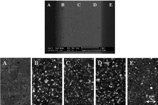
Generally speaking, the ultimate goal of every design is a product which fully utilizes properties of materials used in its construction. This philosophy, in its vast context, naturally leads to an appearance of multi-phase composites with microstructure adapted to operation conditions; e.g. [Petrtýl et al., 1996, Bendsøe and Sigmund, 2004, Ray et al., 2005]. Functionally graded materials (FGMs) present one important man-made class of such material systems. Since their introduction in 1984 in Japan as barrier materials for high-temperature components, FGMs have proved to be an attractive choice for numerous applications such as wear resistant coatings, optical fibers, electrical razor blades and biomedical tools [Neubrand and Rodel, 1997, Uemura, 2003]. To provide a concrete example, consider a microstructure of Al2O3/Y-ZrO2 ceramics (Figure 1) engineered for the production of all-ceramic hip bearings. In this case, controlled composition and porosity allow to achieve better long-term performance and hence lower clinical risks when compared to traditional metallic materials [Lukáš et al., 2005].
As typical of all composites, the analysis of functionally graded materials is complicated by the fact that the explicit discrete modeling of the material microstructure results in a problem which is intractable due to huge number of degrees of freedom and/or its intrinsic randomness. As the most straightforward answer to this obstacle, models with a given smoothly varying material data are often employed. When the spatial non-homogeneity is assumed to follow a sufficiently simple form, this premise opens the route to very efficient numerical schemes, such as specialized finite elements [Santare and Lambros, 2000], boundary element techniques [Sutradhar and Paulino, 2004], meshless methods [Ching and Chen, 2007] or local integral equations [Sládek et al., 2005]. Thanks to their simplicity, these methods can be rather easily generalized to more complex issues such as coupled thermal-mechanical problems [Noda, 1999] or crack propagation [Sekhar et al., 2005]. Although this approach is very appealing from the computational point of view, its validity remains rather questionable as it contains no direct link with the underlying heterogeneous microstructure.
One possibility of establishing such a connection is to assert that the FGM locally behaves as a homogeneous composite characterized by a given volume fraction distribution and use well-established local effective media theories; see, reviews by [Milton, 2002, Böhm, 2005] for more details. Local averaging techniques have acquired a considerable attention due to their simplicity comparable with the previous class of models; see, e.g. [Markworth et al., 1995, Cho and Ha, 2001] for an overview and comparison of various local micro-mechanical models in the context of FGMs. An exemplar illustration of capabilities of this modeling paradigm is the work [Goupee and Vel, 2006] which provides an efficient algorithm for FGMs composition optimization when taking into account coupled thermo-mechanical effects. Still, despite a substantial improvement in physical relevance of the model, local averaging methods may lead to inaccurate results. This was demonstrated by systematic studies of [Reiter et al., 1997] and [Reiter and Dvorak, 1998], which clearly show that the local averaging technique needs to be adapted to detailed character of the microstructure in a neighborhood of the analyzed material point. When considering the local averaging techniques, however, such information is evidently not available as all the microstructural data has been lumped to volume fractions only.
Another appealing approach to FGM modeling is an adaptive discrete modeling of the structure. In order to avoid the fully detailed problem, a simplified model based on, e.g., local averaging techniques is solved first. Then, in regions where the influence of the discreteness of the microstructure is most pronounced, the microstructure with all details is recovered to obtain an accurate solution. Such a modeling strategy has been, e.g., adopted in [Grujicic and Zhang, 1998] when using the Voronoi cell finite element method introduced by [Ghosh et al., 1995] or recently in [Vemaganti and Deshmukh, 2006] in the framework of goal-oriented modeling. Without a doubt, this approach yields the most accurate results for a given distribution of phases. However, its extension to include inevitable randomness of the microstructure seems to be an open problem.
The systematic treatment of FGMs as random, statistically non-homogeneous composites offers, on the other hand, a possibility to apply the machinery of statistical continuum mechanics [Beran, 1968, Torquato, 2001]. In this framework, overall response of the media is interpreted using the ensemble, rather then spatial, averages of the involved quantities. The first class of methods stems from the description of the material composition by a non-stationary random field. This approach was pioneered by [Ferrante and Graham-Brady, 2005] and further refined in [Rahman and Chakraborty, 2007], where the random field description was applied to the volume fractions of the involved phases and the overall statistics was obtained using the local averaging methods. Such a strategy, however, inevitably leads to the same difficulties as in the case of deterministic analysis with a given variation of volume fractions. Alternative methods exploit the tools of mechanics of heterogeneous media. This gives rise to a correct treatment of non-local effects when combined with appropriate techniques for estimating statistics of local fields. Examples of FGMs-oriented studies include the work of [Buryachenko and Rammerstorfer, 2001] who employ the multi-particle effective field method or the study by [Luciano and Willis, 2004] based on the Hashin-Shtrikman energy principles; see also [Buryachenko, 2007] for a comprehensive list of references in this field. Both works, however, being analytically based, concentrate on deriving explicit constitutive equations for FGMs and therefore work with infinite bodies neglecting the finite size of the microstructure.
The goal of this paper is to make the first step in formulating a numerical model which is free of the above discussed limitations. The microstructural description is systematically derived from a fully penetrable sphere model introduced by [Quintanilla and Torquato, 1997], which is briefly reviewed in Section 2. The statistics of local fields then follow from re-formulation of the Hashin-Shtrikman (H-S) variational principles introduced, e.g., in [Willis, 1977, Willis, 1981] and summarized in the current context in Section 3 together with the Galerkin scheme allowing to treat general bodies proposed by [Luciano and Willis, 2005] or [Procházka and Šejnoha, 2003]. Section 4 covers the application of the Finite Element Method (FEM) following [Luciano and Willis, 2005, Luciano and Willis, 2006] and the Boundary Element Method (BEM) in the spirit of [Procházka and Šejnoha, 2003]. Finally, based on results of a parametric study executed in Section 5, the comparison of both numerical scheme when applied to FGMs modeling is performed in Section 6 together with a discussion of future improvements of the model. In order to make the presentation self-contained and to minimize technicalities, the attention is restricted to an one-dimensional elasticity problem (or, equivalently, to a simple laminate subject to body forces varying in one direction; cf. [Luciano and Willis, 2001]).
In the following text, we adopt the matrix notation commonly used in the finite element literature. Hence, , and denote a scalar quantity, a vector (column matrix) and a general matrix, respectively. Other symbols and abbreviations are introduced in the text as needed.
2. Microstructural model
As already indicated in the introductory part, the morphological description adopted in this work is the one-dimensional case of a microstructural model studied in [Quintanilla and Torquato, 1997]. A particular realization can be depicted as a collection on rods of length distributed within a structure of length , see Figure 2. The position of the -th rod is specified by the coordinate of its reference point , which in our case coincides with the midpoint of a rod.

The microstructure gradation is prescribed by an intensity function , with the product giving the expected number of reference points in an infinitesimal neighborhood around . Using the theory of general Poisson processes, the probability of finding exactly points located in a finite-sized interval is given by [Quintanilla and Torquato, 1997]
| with | (1) |
Further, to provide a suitable framework for the description of microstructure related to the model, we attach a symbol to a particular microstructure realization (e.g., Figure 2) from a sample space endowed with a probability measure . Then, the ensemble average of a random function is defined as111To simplify the exposition, we introduce the following notation: for a real-valued random function , by writing we mean a deterministic function of related to a given fixed realization (i.e., ). In other words, it holds .
| (2) |
Now, interpret Figure 2 as a distribution of “white” and “black” phases. For a given configuration , the distribution of a phase is described by the characteristic function
| (3) |
where is reserved for the white phase (matrix) while denotes the black phase (rod). The elementary statistical characterization of the model is provided by the one-point probability function
| (4) |
giving the probability of finding a point included in the phase . Recognizing that the probability of locating in the white phase coincides with the probability that the interval
| (5) |
will not be occupied by any reference point and using Equation (1), we obtain
| (6) |
The one-point probability function follows from the identity
| (7) |
which is a direct consequence of the adopted definition of the characteristic function; recall Equation (3).
By analogy, we can introduce the two-point probability function
| (8) |
quantifying the probability that a point will be located in phase while stays in the phase . For , the descriptor coincides with the probability that the union of intervals and will not be occupied by a reference point, yielding
| (9) |
The remaining functions can be directly expressed from using relations summarized in Appendix A.
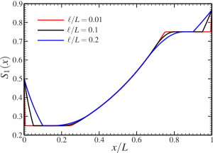
Finally, to provide a concrete example, consider a piecewise linear intensity function
| (10) |
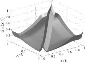
where . The corresponding one- and two-point probability functions, evaluated using an adaptive Simpson quadrature [Gander and Gautschi, 2000], are shown in Figure 3. Obviously, the shape of one-point probability function directly follows from the intensity profile (up to some boundary effects due to extension of by zero outside of and smoothing phenomena with lengthscale demonstrating the ”geometrical” size effect present in the model). The two-point probability function then contains further details of the distribution of individual constituents.
 |
 |
| (a) | (b) |
3. Hashin-Shtrikman variational principles
The introduced geometrical description provides a solid basis for the formulation of a stochastic model of one-dimensional binary functionally graded bodies. In the sequel, we concentrate on the simplest case of linear elasticity with deterministic properties of single components.

3.1. Problem statement
Consider a bar of unit cross-section area, represented by the interval with the boundary , fixed at , subject to a body force and tractions at , see Figure 4. For a given realization , the displacement field follows from the energy minimization problem
| (11) |
where denotes the minimizer of on , is the realization-independent set of kinematically admissible displacements, is a test displacement field and the energy functional is defined as
| (12) |
with the strain field and the Young modulus in the form
| (13) |
where denotes the deterministic Young modulus of the -th phase.
Now, given the probability distribution , the ensemble average of displacement fields follows from the variational problem [Luciano and Willis, 2005]:
| (14) |
In theory, the previous relation fully specifies the distribution of displacement fields. The exact specification of the set is, however, very complex and the probability distribution is generally not known. Therefore, the solution needs to be based on partial geometrical data such as the one- and two-point probability functions introduced in Section 2.
3.2. Hashin-Shtrikman decomposition
Following the seminal ideas of [Hashin and Shtrikman, 1962] and [Willis, 1977], the solution of the stochastic problem is sought as a superposition of two auxiliary problems, each characterized by constant material data .
| (a) | |
|---|---|
| (b) |
In the first ”reference” case, see Figure 5(a), the homogeneous structure is subject to the body force and the boundary tractions . The second ”polarization problem”, shown in Figure 5(b), corresponds to a homogeneous body loaded by polarization stress arising from the stress equivalence conditions:
| (15) |
The unknown polarization stress now becomes a new variable to be determined as the stationary point of the two-field Hashin-Shtrikman-Willis functional; e.g. [Willis, 1977, Procházka and Šejnoha, 2004] and [Bittnar and Šejnoha, 1996, Chapter 1.8]
| (16) |
where denotes an admissible polarization stress from the realization-dependent set , stands for a stationary point of on and a new energy functional is defined as
The minimization with respect to in Equation (16) can be efficiently performed using Green’s function technique. To that end, we introduce a decomposition of the displacement field
| (18) |
where solves the reference problem, while denotes the displacement field due to a test stress polarization field . Note that the determination of is a standard task, which can be generally solved by a suitable numerical technique (cf. Sections 4.1 and 4.2). By introducing the Green function of the reference problem satisfying
| (19) |
with boundary conditions ( denotes the outer normal, recall Figure 5)
| (20) |
we relate the component and the associated strain field
to the polarization stresses via,
cf. [Luciano and Willis, 2005],
| (21) | |||||
| (22) |
By exploiting the optimality properties of the minimizing displacement and upon exchanging the order of optimization, Equation (3.2) can be, after some steps described in, e.g. [Willis, 1981, Luciano and Willis, 2005], recast solely in terms of the polarizations:
| (23) |
where the “condensed” energy functional is defined as
with denoting the total energy of the reference structure.
With the Hashin-Shtrikman machinery at hand, the stochastic problem introduced by Equation (14) can be solved by repeating the previous arguments in the probabilistic framework. In particular, taking the ensemble average of Equations (18) and (21) yields
| (25) |
where the expectation is a solution of the variational problem
| (26) |
Again, due to limited knowledge of detailed statistical characterization of phase distribution, the previous variational problem can only be solved approximately. In particular, we postulate the following form of polarization stresses:
| (27) |
where and are now the realization-independent polarization stresses related to the -th phase. Plugging the approximation into Equation (26) leads, after some manipulations detailed in e.g. [Willis, 1981, Šejnoha, 2000], to the variational principle
| (28) | |||||
i.e. the ”true” phase polarization stresses satisfy the optimality conditions ()
| (29) |
for arbitrary .
3.3. Discretization
Two ingredients are generally needed to convert conditions (29) to the finite-dimensional system: (i) representation of the reference strain field and the Green function-related quantities and (ii) discretization of the phase polarization stresses. The first step is dealt with in detail in Section 4; now it suffices to consider the approximations
| (30) |
where denotes a parameter related to the discretization of the reference problem.222To be more precise, the goal is not to obtain accurate estimates of the Green function-related operators themselves, but rather to approximate the action of the operators; see Section 5.2 for further discussion.
Next, we reduce Equation (29) to a finite-dimensional format using the standard Galerkin procedure. To that end, we introduce the following discretization of the phase polarization stresses
| (31) |
where is the matrix of (possibly discontinuous) shape functions controlled by the discretization parameter ; and denote the degrees-of-freedom (DOFs) of trial and true polarization stresses, the latter related to the discrete Green function. Introducing the approximations (31) into the variational statement (29) and using the arbitrariness of leads to a system of linear equations
| (32) |
with the individual terms given by ()
| (33) | |||||
| (34) | |||||
| (35) |
Finally, once the approximate values of phase polarization stresses are available, the elementary statistics of the displacement field follow from the discretized form of Equation (25)
| (36) |
Note that additional information such as conditional statistics can be extracted from the polarization fields in post-processing steps similar to Equation (36); see [Luciano and Willis, 2005, Luciano and Willis, 2006] for more details.
4. Reference problem and Green’s function-related quantities
4.1. Finite element method
The solution of the reference problem follows the standard Finite Element procedures, see e.g. [Bittnar and Šejnoha, 1996, Krysl, 2006]. Nevertheless, we briefly repeat the basic steps of the method for the sake of clarity.333Recall that for simplicity, we assume homogeneous Dirichlet boundary conditions only. The treatment of the non-homogeneous data can be found in [Luciano and Willis, 2005, Appendix A]. The reference displacement follows from the identity
| (37) |
which should hold for any test function . Within the conforming finite element approach, the unknown displacement and the test function together with the associated strain field are sought in a finite-dimensional subspace
| (38) | |||||
| (39) |
where is the displacement interpolation matrix and denotes the displacement-to-strain matrix. Using the discretized fields, Equation (37) reduces to the system
| (40) |
where
| (41) | |||||
| (42) |
Solving the system for enables us to obtain the approximation using Equation (39)1.
4.2. Boundary element discretization
Following the standard Boundary Element Method procedures (e.g. [Bittnar and Šejnoha, 1996, Duddeck, 2002]), we start from the Betti identity written for the reference problem:
| (46) |
and apply the test displacement in the form
| (47) |
where is the infinite body Green’s function defined as the solution of
| (48) |
In the one-dimensional setting, this quantity is provided by e.g. [Luciano and Willis, 2001, Eq. (13)]
| (49) |
and the integral identity (46), written for any , receives the form:
| (50) |
where the tractions are defined analogously to Equation (20)2:
| for | (51) |
and denotes the Heaviside function. Imposing the consistency with boundary data for and yields the system of two linear equations
| (52) | |||||
| (53) |
Since one component of the pair is always specified on and , the previous system uniquely determines the unknown boundary data (i.e. on and on ), needed to evaluate Equation (50).444It can be verified that Equation (50) now provides the exact one-dimensional displacement field rather than an approximate one. Nevertheless, to keep the following discussion valid in the multi-dimensional setting and consistent with Section 4.1, we keep the index “” in the sequel.
Making use of the identity , the associated strain field can be expressed as
| (54) | |||||
Analogously to the Finite Element treatment, the expression for the finite-body Green function starts from Equation (46) with and boundary data (20). Following the specific form of Equation (50) (and allowing for a slight inconsistency in notation), we introduce a decomposition of the Green function into the discretization-independent infinite-body part and the discretization-dependent boundary contribution:
| (55) |
where the boundary part, written for and , assumes the form
| (56) |
with the boundary displacements and tractions at due to a unit impulse at determined from a linear system (compare with Equations (52) and (53))
| (57) | |||||
| (58) |
Expression for is derived following an analogous procedure. We exploit the infinite-body–boundary split
| (59) |
and obtain the first part directly from the definition (21)
| (60) |
The boundary-dependent part now follows from
| (61) |
with the -sensitivities of boundary data evaluated from (57)–(58):
| (62) | |||||
| (63) |
The BEM-based approach is completed by approximating function. In particular, we get
| (64) | |||||
| (65) | |||||
| (66) | |||||
Finally note that the previous procedure can be directly translated to multi-dimensional and/or vectorial cases; see [Procházka and Šejnoha, 2003, Section 3] for more details.
5. Numerical examples
Before getting to the heart of the matter, we start with converting the relations (32)–(36) into the fully discrete format by replacing the integrals by a numerical quadrature and selecting a specific form of shape functions . To that end, we introduce a set of integration points as well as associated integration weights and evaluate the components of the system matrix and right-hand side vector as
| (67) | |||||
| (68) | |||||
| (69) | |||||
| (70) | |||||
with the convention for the FEM-based approximation of the polarization problem. The basis functions and integration schemes employed in the sequel, based on a uniform partitioning of into cells of length , are defined by Figure 6. In particular, the specification of the polarization stress in terms of shape functions requires DOFs (i.e. one DOF per cell and phase), while and discretizations are parametrized using or values, respectively.
(a) 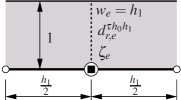 (b)
(b) 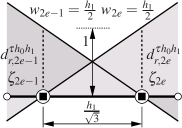 (c)
(c) 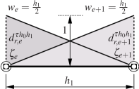
Note that the BEM-related infinite-body contributions appearing in Equations (68) and (70) are still kept explicit, as they are available in the closed form and can be treated separately. In the present case, action of the operator is local (recall Equation (66)), while the quantities related to are evaluated at cell nodal points and linearly interpolated to the interior of a cell to account for the discontinuity of the integrand.
To summarize, the following factors significantly influence the accuracy of the discrete Hashin-Shtrikman scheme:
-
•
approximation of the Green function of the comparison body,
-
•
basis functions and numerical quadrature used to discretize the polarization problem,
-
•
Young’s modulus of the reference body ,
-
•
contrast of the Young moduli of individual phases (),
-
•
characteristic size of microstructure with respect to the analyzed domain ().
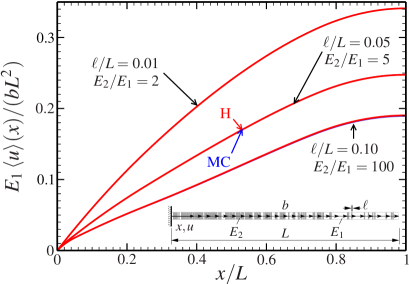
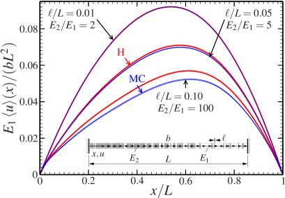
All these aspects are studied in detail in the rest of this Section. Two representative examples of structures subject to a uniform body force and homogeneous mixed and Dirichlet boundary data are considered, see Figure 7:
| statically determinate structure | (71) | ||||
| statically indeterminate structure | (72) |
In both cases, the heterogeneity distribution is quantified according to the model introduced in Section 2 with the one- and two-point probability functions plotted in Figure 3. Moreover, taking advantage of the one-dimensional setting, we systematically compare the obtained numerical results against reliable reference values determined by extensive Monte-Carlo (MC) simulations introduced next.
5.1. Direct simulation results
For the purpose of the following discussion, the reference values of the average displacement fields together with the interval estimates are understood as the piecewise linear interpolants of discrete data sampled by MC procedure described in detail in Appendix B. In addition, the homogenized displacement field , corresponding to a deterministic structure with the position-dependent elastic modulus
| (73) |
is introduced to asses the performance of the local averaging approach. Figure 7 stores several representative results plotted using dimensionless quantities.
 |
 |
| (a) | (b) |
As apparent from Figure 7, the obtained statistics of overall response exhibits rather narrow confidence intervals, implying the reliability and accuracy of the MC estimates. For the statically determinate structure, the locally homogenized solution coincides with the ensemble average of the displacement fields, as demonstrated by the overlap of simulation results with homogenized data. The converse is true (with the confidence) for the statically indeterminate case, where these two results can be visually distinguished from each other. The mismatch (which increases with increasing or ) clearly demonstrates that even in the one-dimensional setting the local averaging may lead to incorrect values when treating non-homogeneous random media. These results are consistent with the fact that in the statically determinate case, the stress field is independent of as follows from the the one-dimensional equilibrium equations and the deterministic value of traction at due to boundary condition provided by Equation (71)2. In the latter case, however, the traction value as well as stress field become configuration-dependent. Such effect does not appear in the classical homogenization setting, where for the harmonic average is known to represent the homogenized solution exactly, cf. [Murat and Tartar, 1997]. This result naturally justifies the application of approaches based on higher-order statistics to FGMs, with the H-S method being the most prominent example.
5.2. Effect of the Green function approximation
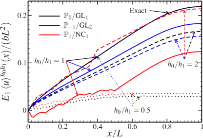
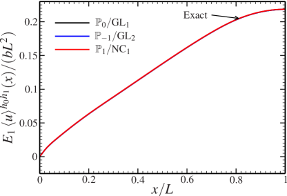
In order to illustrate the effect of approximate Green’s function, we restrict our attention to the statistically determinate structure and employ the standard piecewise linear basis functions to evaluate function in the FEM setting using Equation (45). Figure 8 allows us to perform the qualitative assessment of the results for different choices of basis functions, the integration scheme and the discretization parameter .
 |
 |
| (a) | (b) |
Evidently, a suitable choice of discretization parameter is far from being straightforward. From all the possibilities presented in Figure 8(a), only the combinations with discretization of the polarization problem and with scheme are capable of reproducing the homogenized solution, while all the remaining possibilities lead to inaccurate results often accompanied by an oscillatory response. On the other hand, the -independent BEM-based solutions show correct response for all discretizations of the polarization problem (and are virtually independent of the scheme used due to sufficiently low value of parameter, cf. Section 5.5).
(a) 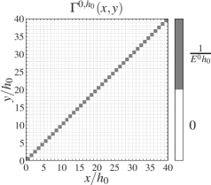
|
(b) 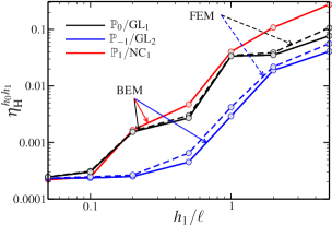
|
To shed a light on such phenomenon, consider the FEM approximation of function plotted in Figure 9(a). The piecewise linear basis functions used to express the reference displacements imply the piecewise constant values of approximating the exact expression , cf. Equation (64). As pointed out by [Luciano and Willis, 2006], however, the accuracy of the HS scheme is governed by the correct reproduction of the action of the operator rather than the local values. In the present context, it follows from Equation (69) that such requirement is equivalent to the accurate representation of the operator action for coinciding with the integration points related to the selected numerical quadrature. It can be verified that this condition is satisfied only for the two aforementioned discretizations of the reference problem. In particular, for the combination we obtain (see Figures 9(a) and 10(a))
| (74) |
i.e. the numerical scheme reproduces the action of exactly.
Using Figures 9(a) and 10(b), we find the analysis of the discretization completely analogous:
| (75) |
which explains the good performance of the particular discretization scheme.
(a) 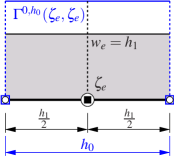 (b)
(b) 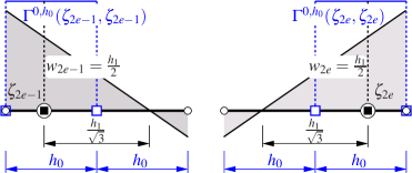
To allow for the quantitative comparison, we exploit the fact that the exact solution is available for the statically determinate case and introduce a relative error measure
| (76) |
The resulting convergence rates of the FEM- and BEM-based approach are shown in Figure 10(b) with integrals in Equation (76) evaluated using an adaptive Simpson quadrature [Gander and Gautschi, 2000] with the relative accuracy of . Clearly, the performance of the BEM-based scheme is slightly superior to the (properly “tuned”) FEM approach. By a sufficient resolution of the reference problem, however, both approaches become comparable. Moreover, the results confirm good performance of and schemes when compared to the discretization, which requires about twice the number of DOFs of former schemes for the same cell dimensions (recall Figure 6). Similar conclusions can also be drawn for the statically indeterminate case. Therefore, in view of the above comments, we concentrate on the BEM approach in the sequel and limit the choice of basis functions to and only.
5.3. Influence of the integration scheme and basis functions
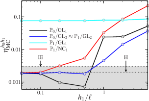
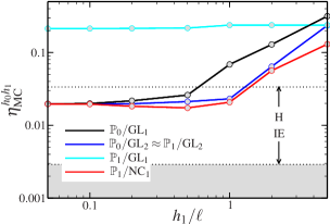
Thus far, we have investigated the combination of the “polarization” numerical quadratures and shape functions, for which the location of integration points coincides with the position of DOFs. Figure 11 shows the convergence plots for the relevant basis function/integration scheme pairs. To address also the statically determinate case, the relative error is now related to MC data, leading to the definition
| (77) |
In addition, two comparative values are introduced: the relative error of the homogenized solution (determined by Equation (77) with replaced by ) and the relative error associated with or function, appearing as the Interval Estimate (IE) line.
 |
 |
| (a) | (b) |
For the statistically determinate structure, the observed behavior is rather similar to the one reported in Section 5.2. In particular, Figure 11(a) confirms that the H-S solution quickly reaches the accuracy comparable with the confidence intervals (indicated by the grey area) and eventually converges to the homogenized solution, with the exception of combination resulting in a singular system matrix (32). Moreover, the superiority of the quadrature over lower-order scheme is evident; the proper representation of spatial statistics seems to be more important than smoothness of the polarization shape functions.
Figure 11(b) shows the results for the statically indeterminate case. With confidence, the results quantitatively demonstrate that the homogenized solution differs from the MC data. The H-S solution gives the error about of the value of the homogenized solution, but ceases to attain the accuracy set by the confidence interval. It should be kept in mind that the H-S result actually delivers an estimate pertinent to the fixed value of parameter and all random one-dimensional media characterized by the two-point statistics (9).
5.4. Influence of the reference media and phase contrast
Having identified the intrinsic limitation of the H-S approach, we proceed with the last free parameter of the method: the choice of the reference medium. To that end, we introduce the following parameterization of the Young modulus
| (78) |
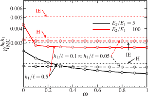
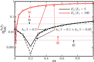
Note that for the phases indexed such that , and correspond to the rigorous lower and upper bounds on the ensemble average of the energy stored in the structure and, consequently, to the positive- or negative-definite system matrix [Procházka and Šejnoha, 2004, Luciano and Willis, 2005]. The intermediate values lead to energetic variational estimates and to a symmetric indefinite system matrix. Figure 12 illuminates the effect of , plotted for two representative contrasts of phase moduli and ratios.
 |
 |
| (a) | (b) |
In the first case, see Figure 12(a), the choice of the reference media has almost negligible effect on the H-S solution error; the slight influence observed for the coarse discretization completely disappears upon cell refinement. This is not very surprising as the homogenized solution depends on the first-order statistics only, recall Equation (73), and as such can be retained by the discrete H-S method (up to controllable errors) for any choice of . Results for the statically indeterminate structure, on the other hand, show a significant sensitivity to the value of . By a proper adjustment of the reference medium, the error can be reduced by an order of magnitude and eventually reach the accuracy of extensive MC sampling. With increasing phase moduli contrast, however, the range of such values rapidly decreases; for one needs to satisfy in order to recover the MC results. It is noteworthy that these values agree rather well with the particular choice of reference media used by [Matouš, 2003] when modeling composites with a high phase contrast using the methodology proposed by [Dvorak and Srinivas, 1999].
5.5. Influence of microstructure size
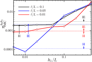
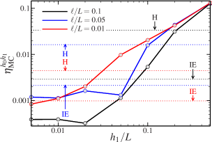
Eventually, we investigate the influence of the microstructure size. Figure 13 summarizes the obtained results for a moderate phase contrast and the optimal setting of the H-S method identified in the previous sections. A similar conclusion can be reached for the both case studies: for all three values, the H-S method is capable of reaching the accuracy of MC confidence intervals for the cell length approximately equal to a half of the microscopic lengthscale . In other words, keeping the same number of DOFs as used to discretize the polarization problem, the accuracy of the method increases with the increasing ratio, which is exactly an opposite trend to that of the classical deterministic homogenization.
 |
 |
| (a) | (b) |
6. Conclusions
In the present work, the predictive capacities of numerical methods based on the Hashin-Shtrikman-Willis variational principles, when applied to a specific model of functionally graded materials, have been systematically assessed. By restricting attention to the one-dimensional setting, an extensive parametric study has been executed and the results of numerical schemes have been verified against reliable large-scale Monte-Carlo simulations. On the basis of obtained data, we are justified to state that:
-
•
The Hashin-Shtrikman based numerical method, when set up properly, is capable of delivering results with the accuracy comparable to detailed Monte Carlo simulations and, consequently, of outperforming the local averaging schemes.
-
•
When applying the Finite Element method to the solution of reference problem, the employed discretization has to be compatible with the numerics used to solve the polarization problem. If this condition is satisfied, the additional FEM-induced errors quickly become irrelevant.
-
•
For the discretization of the reference problem, it appears to be advantageous to combine low order (discontinuous) approximation of the polarization stresses with higher order quadrature scheme to concisely capture the heterogeneity distribution.
-
•
The correct choice of the reference medium has the potential to substantially decrease the error. Unfortunately, apart from [Dvorak and Srinivas, 1999], we fail to give any a-priory estimates of the optimal value for statistically non-homogeneous structures.
-
•
For accurate results, the characteristic cell size should be around – times smaller than the typical dimensions of the constituents.
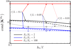
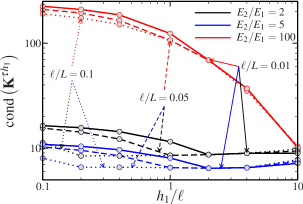
The bottleneck of the current implementation is the solution of system (32), since it leads to a fully populated system matrix. Fortunately, as illustrated by Figure 14, the conditioning of the polarization problem seems to be dominated by the phase contrast rather than the discretization of the reference problem, which opens the way to efficient iterative techniques.
 |
 |
| (a) | (b) |
The next extension of the method would involve the generalization to the multi-dimensional setting. For the FEM-based treatment, the key aspect remains a more rigorous analysis of the combined effect of discretized operator, basis functions and integration scheme employed for the polarization problem. The multi-dimensional BEM approach, on the other hand, requires a careful treatment of singularities of the Green function-related quantities, cf. [Procházka and Šejnoha, 2003], which are suppressed in the current one-dimensional setting. Such work will be reported separately in our future publications.
Acknowledgments
We would like to thank Jiří Šejnoha, Michal Šejnoha, Jan Novák and Milan Jirásek for numerous discussions on the topic of this work. The first authoress acknowledges the support from project No. 103/07/0304 (GA ČR), the work of the second author was supported from the research project MSM 6840770003 (MŠMT ČR).
References
- [Bendsøe and Sigmund, 2004] Bendsøe, M. and Sigmund, O. (2004). Topology optimization. Springer, second edition.
- [Beran, 1968] Beran, M. J. (1968). Statistical Continuum Theories. Monographs in Statistical Physics. Interscience Publishers.
- [Bittnar and Šejnoha, 1996] Bittnar, Z. and Šejnoha, J. (1996). Numerical methods in structural mechanics. ASCE Press and Thomas Telford, Ltd, New York and London.
-
[Böhm, 2005]
Böhm, H. (2005).
A short introduction to basic aspects of continuum micromechanics.
Technical Report hjb/ILSB 050103, Christian Doppler Laboratory for
Functionally Oriented Materials Design, Institute of Lightweight Design and
Structural Biomechanics, Vienna University of Technology.
http://www.ilsb.tuwien.ac.at/links/downloads/cdlfmdrep03.pdf (07/01/2008). - [Buryachenko, 2007] Buryachenko, V. (2007). Micromechanics of Heterogeneous Materials. Springer.
- [Buryachenko and Rammerstorfer, 2001] Buryachenko, V. and Rammerstorfer, F. (2001). Local effective thermoelastic properties of graded random structure matrix composites. Archive of Applied Mechanics, 71(4–5):249–272.
- [Ching and Chen, 2007] Ching, H. K. and Chen, J. K. (2007). Thermal stress analysis of functionally graded composites with temperature-dependent material properties. Journal of Mechanics of Materials and Structures, 2(4):633–653.
- [Cho and Ha, 2001] Cho, J. R. and Ha, D. Y. (2001). Averaging and finite-element discretization approaches in the numerical analysis of functionally graded materials. Materials Science and Engineering A, 302(2):187–196.
- [Duddeck, 2002] Duddeck, F. M. E. (2002). Fourier BEM: Generalization of Boundary Element Methods by Fourier transform, volume 5 of Lecture Notes in Applied Mechanics. Springer Verlag, Berlin, Heidelberg, New York.
- [Dvorak and Srinivas, 1999] Dvorak, G. J. and Srinivas, M. V. (1999). New estimates of overall properties of heterogeneous solids. Journal of the Mechanics and Physics of Solids, 47(4):899–920.
- [Ferrante and Graham-Brady, 2005] Ferrante, F. J. and Graham-Brady, L. L. (2005). Stochastic simulation of non-gaussian/non-stationary properties in a functionally graded plate. Computer Methods in Applied Mechanics and Engineering, 194(12–16):1675–1692.
- [Gander and Gautschi, 2000] Gander, W. and Gautschi, W. (2000). Adaptive quadrature–Revisited. BIT Numerical Mathematics, 40(1):84–101.
- [Ghosh et al., 1995] Ghosh, S., Lee, K., and Moorthy, S. (1995). Multiple scale analysis of heterogeneous elastic structures using homogenization theory and Voronoi cell finite element method. International Journal of Solids and Structures, 32(1):27–62.
- [Goupee and Vel, 2006] Goupee, A. J. and Vel, S. S. (2006). Two-dimensional optimization of material composition of functionally graded materials using meshless analyses and a genetic algorithm. Computer Methods in Applied Mechanics and Engineering, 195(44–47):5926–5948.
- [Grujicic and Zhang, 1998] Grujicic, M. and Zhang, Y. (1998). Determination of effective elastic properties of functionally graded materials using Voronoi cell finite element method. Materials Science and Engineering A-Structural Materials Properties Microstructure and Processing, 251(1–2):64–76.
- [Hashin and Shtrikman, 1962] Hashin, Z. and Shtrikman, S. (1962). On some variational principles in anisotropic and nonhomogeneous elasticity. Journal of the Mechanics and Physics of Solids, 10(4):185–202.
- [Higham and Tisseur, 2000] Higham, N. J. and Tisseur, F. (2000). A block algorithm for matrix 1-norm estimation, with an application to 1-norm pseudospectra. SIAM Journal on Matrix Analysis and Applications, 21(4):1185–1201.
- [Krysl, 2006] Krysl, P. (2006). A pragmatic introduction to the Finite Element Method for thermal and stress analysis. World Scientific Publishing.
- [Luciano and Willis, 2004] Luciano, R. and Willis, J. (2004). Non-local constitutive equations for functionally graded materials. Mechanics of Materials, 36(12):1195–1206.
- [Luciano and Willis, 2005] Luciano, R. and Willis, J. (2005). FE analysis of stress and strain fields in finite random composite bodies. Journal of the Mechanics and Physics of Solids, 53(7):1505–1522.
- [Luciano and Willis, 2006] Luciano, R. and Willis, J. (2006). Hashin-Shtrikman based FE analysis of the elastic behaviour of finite random composite bodies. International Journal of Fracture, 137(1–4):261–273.
- [Luciano and Willis, 2001] Luciano, R. and Willis, J. R. (2001). Non-local constitutive response of a random laminate subjected to configuration-dependent body force. Journal of the Mechanics and Physics of Solids, 49:431–444.
- [Lukáš et al., 2005] Lukáš, P., Vrána, M., Šaroun, J., Ryukhtin, V., Vleugels, J., Anne, G., Van der Biest, O., and Gasik, M. (2005). Neutron diffraction studies of functionally graded alumina/zirconia ceramics. Materials Science Forum, 492–493:201–206.
- [Markworth et al., 1995] Markworth, A., Ramesh, K., and Parks, W. (1995). Modeling studies applied to functionally graded materials. Journal of Materials Science, 30(9):2183–2193.
- [Matouš, 2003] Matouš, K. (2003). Damage evolution in particulate composite materials. International Journal of Solids and Structures, 40(6):1489–1503.
- [Milton, 2002] Milton, G. W. (2002). The Theory of Composites, volume 6 of Cambridge Monographs on Applied and Computational Mathematics. Cambridge University Press.
- [Murat and Tartar, 1997] Murat, F. and Tartar, L. (1997). Calculus of variations and homogenization. In Cherkaev, A. and Kohn, R., editors, Topics in Mathematic Modelling of Composite Materials, number 31 in Progress in Nonlinear Differential Equations and Their Applications, pages 139–173. Birkhäuser, Boston.
- [Neubrand and Rodel, 1997] Neubrand, A. and Rodel, J. (1997). Gradient materials: An overview of a novel concept. Zeitschrift für Metallkunde, 88(5):358–371.
- [Noda, 1999] Noda, N. (1999). Thermal stresses in functionally graded materials. Journal of Thermal Stresses, 22(4–5):477–512.
- [Petrtýl et al., 1996] Petrtýl, M., Hert, J., and Fiala, P. (1996). Spatial organization of the haversian bone in man. Journal of Biomechanics, 29(2):161–167.
- [Procházka and Šejnoha, 2003] Procházka, P. and Šejnoha, J. (2003). A BEM formulation for homogenization of composites with randomly distributed fibers. Engineering Analysis with Boundary Elements, 27(2):137–144.
- [Procházka and Šejnoha, 2004] Procházka, P. and Šejnoha, J. (2004). Extended Hashin-Shtrikman variational principles. Applications of Mathematics, 49(4):357–372.
- [Quintanilla and Torquato, 1997] Quintanilla, J. and Torquato, S. (1997). Microstructure functions for a model of statistically inhomogeneous random media. Physical Review E, 55(2):1558–1565.
- [Rahman and Chakraborty, 2007] Rahman, S. and Chakraborty, A. (2007). A stochastic micromechanical model for elastic properties of functionally graded materials. Mechanics of Materials, 39(6):548–563.
- [Ray et al., 2005] Ray, A., Mondal, S., Das, S., and Ramachandrarao, P. (2005). Bamboo - A functionally graded composite-correlation between microstructure and mechanical strength. Journal of Materials Science, 40(19):5249–5253.
- [Reiter and Dvorak, 1998] Reiter, T. and Dvorak, G. (1998). Micromechanical models for graded composite materials: II. Thermomechanical loading. Journal of the Mechanics and Physics of Solids, 46(9):1655–1673.
- [Reiter et al., 1997] Reiter, T., Dvorak, G., and Tvergaard, V. (1997). Micromechanical models for graded composite materials. Journal of the Mechanics and Physics of Solids, 45(8):1281–1302.
- [Rektorys, 1994] Rektorys, K., editor (1994). Survey of applicable mathematics: Volume II, volume 281 of Mathematics and its Applications. Kluwer Academic Publishers Group, Dordrecht, second revised edition.
- [Santare and Lambros, 2000] Santare, M. and Lambros, J. (2000). Use of graded finite elements to model the behavior of nonhomogeneous materials. Journal of Applied Mechanics-Transactions of the ASME, 67(4):819–822.
- [Sekhar et al., 2005] Sekhar, S., Kandula, V., Abanto-Bueno, J., Geubelle, P. H., and Lambros, J. (2005). Cohesive modeling of dynamic fracture in functionally graded materials. International Journal of Fracture, 132(3):275–296.
- [Sládek et al., 2005] Sládek, V., Sládek, J., and Zhang, C. (2005). Domain element local integral equation method for potential problems in anisotropic and functionally graded materials. Computational Mechanics, 37(1):78–85.
- [Stoyan et al., 1987] Stoyan, D., Kendall, W., and Mecke, J. (1987). Stochastic Geometry and Its Applications. Akademie-Verlag, Berlin.
- [Sutradhar and Paulino, 2004] Sutradhar, A. and Paulino, G. (2004). The simple boundary element method for transient heat conduction in functionally graded materials. Computer Methods in Applied Mechanics and Engineering, 193(42–44):4511–4539.
- [Torquato, 2001] Torquato, S. (2001). Random heterogeneous materials: Microstructure and macroscopic properties. Springer-Verlag.
- [Uemura, 2003] Uemura, S. (2003). The activities of FGM on new application. Materials Science Forum, 423–425:1–10.
- [Vemaganti and Deshmukh, 2006] Vemaganti, K. and Deshmukh, P. (2006). An adaptive global-local approach to modeling functionally graded materials. Computer Methods in Applied Mechanics and Engineering, 195(33–36):4230–4243.
- [Šejnoha, 2000] Šejnoha, M. (2000). Micromechanical analysis of random composites. Habilitation thesis, Faculty of Civil Engineering, Czech Technical University in Prague. http://mech.fsv.cvut.cz/~sejnom/download/hab.pdf.
- [Willis, 1977] Willis, J. R. (1977). Bounds and self-consistent estimates for the overall properties of anisotropic composites. Journal of the Mechanics and Physics of Solids, 25(3):185–202.
- [Willis, 1981] Willis, J. R. (1981). Variational and related methods for the overall properties of composites. In Advances in Applied Mechanics, volume 21, pages 2–74.
Appendix A Two-point probability functions
The remaining two-point probability functions can be easily related to by exploiting the identity (7). In particular, we obtain
| (79) | |||||
| (80) | |||||
| (81) |
Appendix B Overview of the simulation procedure
A crude Monte-Carlo method is employed to estimate the statistics of the local fields. In particular, given a number of simulations , sampling points and an upper bound on the intensity , the following steps are repeated for :
- Microstructure generation:
-
Construction of a microstructural samples is based on a two-step procedure proposed for general Poisson processes in [Stoyan et al., 1987, Section 2.6]. First, the number of reference points is determined by simulating a Poisson random variable with the mean . The coordinates of the reference points then follow from a realization of independent random variables uniformly distributed on a closed interval . Second, each point in the set is deleted with a probability , leading to a (relabeled) sequence of particle centers .
- Solution of the one-dimensional problem:
-
With the microstructure realization fixed, the displacement of sampling points is computed by the recursion
(82) where the Young modulus is provided by Equation (13) with the characteristic function defined as
and the boundary data and determined from a generalization of the system of boundary equations (52)–(53).
After completing the sampling phase, the first and second-order local statistics are assessed using the unbiased values
to arrive at the -confidence interval estimates, cf. [Rektorys, 1994, Section 34.8]:
| (83) | |||||
where denotes the inverse of the Student distribution function for value and degrees of freedom.
The reference results reported in Section 5 correspond to the values obtained for simulations, the confidence level , equidistant sampling points and the integral (82) evaluated with an adaptive Simpson quadrature [Gander and Gautschi, 2000] with the relative tolerance set to .