How to use magnetic field information for coronal loop identification?

Abstract

The structure of the solar corona is dominated by the magnetic field because the magnetic pressure is about four orders of magnitude higher than the plasma pressure. Due to the high conductivity the emitting coronal plasma (visible e.g. in SOHO/EIT) outlines the magnetic field lines. The gradient of the emitting plasma structures is significantly lower parallel to the magnetic field lines than in the perpendicular direction. Consequently information regarding the coronal magnetic field can be used for the interpretation of coronal plasma structures. We extrapolate the coronal magnetic field from photospheric magnetic field measurements into the corona. The extrapolation method depends on assumptions regarding coronal currents, e.g. potential fields (current free) or force-free fields (current parallel to magnetic field). As a next step we project the reconstructed 3D magnetic field lines on an EIT-image and compare with the emitting plasma structures. Coronal loops are identified as closed magnetic field lines with a high emissivity in EIT and a small gradient of the emissivity along the magnetic field.

Appl. Opt. Kluwer Prepress Department
P.O. Box 990
3300 AZ Dordrecht
The Netherlands

KAPKluwer Academic Publishers; compuscriptElectronically submitted article

KAPKluwer Academic Publishers; compuscriptElectronically submitted article

D24, L60, 047

1 Introduction

The automatic identification of features in solar images provide an increasingly helpful tool for the analysis of solar physics data. Previous methods of solar feature identification used, e.g, contrast, intensity and contiguity criteria in Ca II K images to identify structures like sunspots and plage [Worden, White, & Woods (1998), Preminger, Walton, & Chapman (2001)]. Here we are mainly interested in identifying closed loop structures in active regions. Coronal plasma loops are optical thin and coronal images, e.g. in X-rays or EUV radiation, provide only a 2D projection of the 3D structures. The line-of-sight integrated character of these images complicates their interpretation. The corresponding problem that loop structures visible in images are often a superposition of individual loops occurs particularly in high resolution TRACE images [Schrijver et al. (1999), Schrijver et al. (2004)], although occasionally individual loops are clearly visible over a large fraction of their length [Aschwanden, Nightingale, & Alexander (2000)]. To get insights regarding the structure of the coronal plasma it is important to consider the distribution of the plasma $\beta$ with height. The plasma $\beta$ varies from $\beta>1$ in the photosphere over $\beta\ll 1$ in the mid-corona to $\beta>1$ in the upper corona (See Gary(2001) for details). For the interpretation of coronal loops it is helpful that they are located in the low $\beta$ corona and consequently their structure is dominated by the coronal magnetic field. In the following we will therefore discuss how information about the magnetic field can be used for the analysis of coronal images, e.g., from SOHO/EIT, SOHO/SUMER, or in future from the two STEREO spacecrafts.

The strongest emissivity in EUV-images originates from closed magnetic loops in active regions. Due to the high conductivity the coronal plasma becomes trapped on close magnetic field lines and consequently the emitting plasma outlines the magnetic field Poletto et al. (1975); Sakurai & Uchida (1977); Sakurai (1989). This feature has previously been used (in combination with line of sight photospheric magnetograms) to compute free parameters (e.g., the linear force-free parameter $\alpha$) in coronal magnetic field models. Schrijver et al.(2004) used global potential fields and scaling laws to fill the coronal magnetic field lines with plasma and computed so called synthetic EIT images from their magnetic field model, which they compared with real EIT observations. While potential fields give a rough impression regarding the global structure of the solar corona (e.g. the location of coronal holes and active regions, Neugebauer et al. 2002) they often fail to describe magnetic fields in active regions accurately. Here we use different magnetic field models (potential, force-free fields and coronal magnetic fields reconstructed directly from measurements) in combination with coronal plasma images to identify coronal structures, where we concentrate on closed loops in an active region.

While the space in the corona is basically filled with magnetic field, only some fraction of all field lines shows a strong emissivity. Our aim is to identify out of the many (theoretical infinite) number of field lines the ones which are accompanied by a strong plasma radiation. Aschwanden et al. (1999) picked out individual loops from two EIT images and applied a geometrical fit (assumption of circular loops) and dynamic stereoscopy to draw conclusions regarding the 3D structure of the loops. Wiegelmann & Neukirch (2002) used these circular 3D loops and a MDI magnetogram to compute the optimal linear force-free field consistent with these observations. The method was extended by Carcedo et al. (2003) to work with 2D coronal images, in which an individual loop is visible in coronal images along it’s entire length (including the approximate location of both footpoints). An alternative approach was taken by Marsch, Wiegelmann, & Xia (2004), who identified several loops or (large) parts of loops in EIT-images (by manual tracing). The purpose of these papers was not feature identification, but to use coronal images and line of sight magnetograms to compute the coronal magnetic field within a linear force-free model. A manual selection of the loops was necessary.

The aim of this work is to automize these procedures and allow more general magnetic field models. We use linear and non-linear force-free magnetic field models and also give an example with measured magnetic fields. In the special case of linear force-free fields our method automatically calculates the optimal linear force-free parameter $\alpha$.

In this sense the method is a further development for computing linear force-free fields from line-of sight magnetograms and coronal images. We outline the paper as follows: In section 2 we outline the loop identification method and in section 3 we describe how our method finds the optimal values for magnetic field models with free parameters. Section 4 contains an example where we tested our algorithm with different magnetic field models. Finally we draw conclusions and give an outlook for future work in section 5.

2 The loop identification method

Figure 1: 3D magnetic field of AR7953. We used a linear force-free model with $\alpha=-0.11Mm^{-1}$ to extrapolate photospheric magnetic field measurements into the corona. We plot only closed magnetic field lines with a magnetic field strength above $100G$ at the solar surface. Please note that the vertical scale is stretched by a factor of two.

Figure 2: EIT picture of AR 7953 and projections of linear force-free magnetic field lines. The field lines have been computed with the help of our loop identification method. It is obvious from the pictures that a linear force-free model with a negative value of $\alpha=-0.011Mm^{-1}$ (panel a) fits the EIT-image better than a potential field (panel b) or a linear force-free field with a positive value of $\alpha=0.011Mm^{-1}$ (panel c). Panel d) shows quantitative (value of $C$, see text) agreement of the magnetic field model and EIT-image. The value of $C$ was averaged over the best four individual loops. The error-bars indicate the scatter (standard deviation of $C$ with respect to the four best loops) of the identified structures with respect to the measure $C$.

Previous loop identification methods used the enhanced brightness of coronal loops compared with the background. Klimchuk et al.(1992) and Klimchuk(2000) identified loops by visually selecting the brightest pixels in coronal images and fitting them by least square with a polynomial function. Aschwanden et al. (1999) subtracted a smoothed image (using a $3\times 3$ boxcar) from the original to enhance the loop structure. The key assumption for our method is that the coronal plasma, visible e.g. with EIT, also outlines the coronal magnetic field. Due to the low plasma pressure in the corona the magnetic field dominates the structures of the corona and due to the high conductivity the coronal plasma is trapped on field lines. The method involves the following steps:

1. Compute the coronal magnetic field.

2. Calculate magnetic field lines.

3. Project all magnetic field lines onto an image of the coronal plasma, e.g. from EIT.

4. Compute emissivity and emissivity gradient of the image along the projected field lines.

5. Check how well projected field lines and plasma features agree expressed by a quantitative parameter.

6. Sort loops and choose the best ones in the sense of agreement with the plasma features.

7. Plot some representative loops onto the image.

2.1 Compute the coronal magnetic field.

Direct observations of the coronal magnetic field are only available for a few individual cases (see section 4) and usually one has to extrapolate the coronal magnetic field from photospheric measurements. Full disc line of sight magnetograms are routinely observed with, e.g., SOHO/MDI and at Kitt Peak. Assumptions regarding the coronal current flow are essential for the extrapolation method.

• Current free potential fields can be computed from LOS-magnetograms alone. Potential fields are usually not a good model for magnetic fields in active regions.

• Linear force free fields are also computed from LOS-magnetograms, but contain a free parameter $\alpha$. We will illustrate later, how our method finds the optimal value of $\alpha$, i.e. the one fits the observations best.

• Nonlinear force-free fields require photospheric vector magnetograms as input and are numerically more expensive to compute. If these data are available, nonlinear force-free fields are preferred over linear force-free fields. The reason is that linear force-free fields are a subclass of non-linear force-free fields and consequently non-linear fields provide a larger class of solutions. Unfortunately, current vector magnetograms usually have a limited field of view, large noise in the transversal field component and are simply often not available for active regions of interest. This situation will improve once SOLIS starts providing regular vector magnetograms.

Let us remark that the result of the extrapolation is as well influenced by the lateral and top boundary conditions of the computational box. A popular choice for the upper boundary of global potential fields is a source surface (all field lines are forced to become radial on the source surface.) The extrapolation method of linear force-free fields implicitly specifies the upper boundary by assuming that the magnetic field is bounded at infinity (see Seehafer(1978) for details.) The limited field of view of magnetograms effect the extrapolation as well, because distance sources become neglected and one has to specify lateral boundary conditions, e.g. symmetry assumptions or a boundary layer towards the lateral and top boundaries of the computational box. The effects of the lateral boundary conditions on the reconstruction can be diminished by choosing a well isolated active region with low magnetic flux close to the side boundaries of the computational box (See Wiegelmann(2004 for details). Our method usually uses linear force-free fields, but we will present also one example where we used non-linear force-free fields and coronal magnetic loops deduced directly from spectropolarimetric observations.

2.2 Calculate magnetic field lines.

We use a forth order Runge-Kutta field line tracer to compute a large number of magnetic field lines. The starting points for the field line integration are chosen randomly at the solar surface, whereby the number of traced field lines starting from a given surface area is proportional to the strength of the magnetogram signal. The particular concentration on loops with high magnetic flux is motivated by scaling laws Schrijver et al. (2004) which suggests that loops with a strong magnetic field are also bright loops.

Because the coronal plasma is trapped on closed magnetic loops and has a high emissivity there we are interested here in studying closed magnetic loops. We therefore store only field lines which are closed.

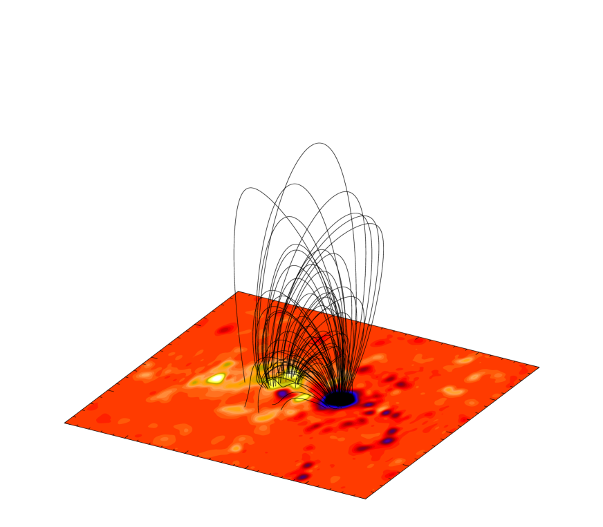
Fig. 1 shows an example. We computed the 3D magnetic field of AR7953 with the help of a linear force-free model using the method of Seehafer (Seehafer) for a linear force-free value of $\alpha=-0.011{\rm Mm}^{-1}$. We plot only closed magnetic field lines where at least one footpoint has $B_{z}>100G$ in the photosphere. The value of the magnetic field is implicit also a threshold for the brightness of the loops and we are interested mainly in identifying bright loops. This is in particular important for the STEREO mission, where we want to identify pairs of loops in two images.

2.3 Project all magnetic field lines onto an image of the coronal plasma, e.g. from EIT.

The faint, optically thin, structure of the coronal emission does not give information regarding its height in the corona. Therefore the 3D magnetic field lines are projected onto an EIT-image on the disk for comparison. It is assumed that the source of high emission is located in closed magnetic structures.

2.4 Compute emissivity and emissivity gradient of the image along the projected field lines.

We compute the emissivity $\rho$ and it’s gradient $\nabla\rho$ along the magnetic field lines. The coronal plasma is assumed to outline the magnetic field and consequently the emissivity gradient parallel to the field lines should be small.

2.5 Check how well projected field lines and plasma features agree.

We use the following measure to get quantitative information on how good a given field line and the plasma emission agree.

$$C=\frac{\int_{0}\limits^{l}|\nabla\rho|\;ds}{l\;\left(\int_{0}\limits^{l}\rho\;ds\right)^{2}}$$ (1)

where $l$ is the length of the loop and the integrals sum along the loop. The lower the value of $C$ the better magnetic loop and plasma agree with each other. One may certainly play around with the exact parameters in Eq. 1, e.g. use simply $\frac{\int_{0}\limits^{l}|\nabla\rho|\;ds}{\int_{0}\limits^{l}\rho\;ds}$ or $\frac{\int_{0}\limits^{l}|\nabla\rho|\;ds}{l\;\int_{0}\limits^{l}\rho\;ds}$. The form used in Eq. 1 gives stronger weight to loops with a high emissivity and long loops. We compute a value of $C$ for all field lines. The gradient along the center of the coronal loop is low but also the gradient could be low far from the loops and the denominator normalization factor may not always correct this if the first potence of the emissivity is used in the nominator. We find that taking the square of the emissivity in the nominator ensures that C becomes large far from the loops and the nominator compensates the low emissivity gradient in the background plasma. The computation of $C$ might become influenced by overlapping and crossing loops which locally enhance the emissivity and the emissivity gradient.

Since any coronal image samples only gas within a limited range of temperatures, this method assumes that coronal loops have a homogeneous temperature along their entire length. This is a relative good approximation (e.g. Brković et al. 2002).

Another possibility to check the agreement between magnetic field lines and the coronal emission is to fit a Gaussian to the coronal plasma perpendicular to the magnetic field lines and to compute the shift between the center of the Gaussian and magnetic field lines integrated along the loop Carcedo et al. (2003). This method was especially successful for single isolated loops, where both footpoint areas of the loop have been identified and only field lines connecting both footpoint areas have been considered for the Gaussian fit. Note that this technique does not rely on the assumption of loops with uniform temperature. Within this work we are planning to automatically detect the loops without any prior footpoint identification. Often one or both footpoints are not visible in the coronal emission. A Gaussian fit can also give misleading results when different coronal loops lie close together in the image.

2.6 Sort loops and choose the best ones in the sense of agreement with the plasma features.

We sort all field lines with respect to the measure $C$. In principle every plasma feature consists of an infinite number of magnetic field lines and after sorting the loops with respect to $C$ it might happen that the best identified loops (lowest values of $C$) lie close together. For the identification and illustration of coronal loops it seems to be better that every feature is only represented by one field line. To do so we compute the difference of all projected field lines (e.g. the area between two field lines) and choose only loops which are clearly separated (area between the loops above a certain threshold).

2.7 Plot some representative loops onto the image.

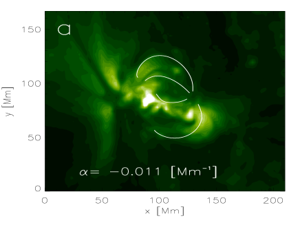
Eventually we plot the projections of the best loops onto the coronal images. Fig. 2 a) shows four identified loops. The alignment of the coronal structures with the magnetic loops is obvious. A more detailed discussion of this figure is given in section 3. Let us remark that our method not only provides the locations of the 2D projection of the loop, but additional information as well. The magnetic field automatically provides the 3D structure of the identified coronal features, the magnetic field strength and current density along the loop. Together with other information from coronal images, e.g. information regarding the plasma flow with SUMER, we can draw further conclusions regarding physical properties. For example Marsch, Wiegelmann, & Xia (2004) studied plasma flows along magnetic field lines for this active region with the help of SUMER data.

3 Using magnetic field models with free parameters

Coronal images give information regarding the direction of the coronal magnetic field. A magnetic field model provides the 3D-magnetic field in the entire space and projections of corresponding magnetic field lines onto the disk can be compared with the coronal image. For non-linear force-free field extrapolations from vector magnetograms or models based on measurements of coronal magnetic fields the projected model field lines are independent from the coronal image. Magnetic field model and coronal image provide independent from each other information regarding the direction of the magnetic field. Unfortunately models based on non-linear force-free extrapolations or direct measurements are currently only available for a few individual cases. Usually the only available magnetic field data are line-of-sight magnetograms from e.g. MDI or Kitt Peak. Under the assumption of current-free potential fields the coronal magnetic field can be derived from LOS-magnetograms. Unfortunately current-free models are usually not a good description for magnetic fields in active regions. We can, however, consider electric currents with the help of linear force-free models where the current free parameter $\alpha$ is unknown a priori and cannot be derived from the LOS-magnetogram. Wiegelmann & Neukirch (2002) used 3D stereoscopic reconstructed loops from Aschwanden et al. (1999) to fix $\alpha$ and Carcedo et al. (2003) fitted $\alpha$ with the help of a plasma loop identified earlier.

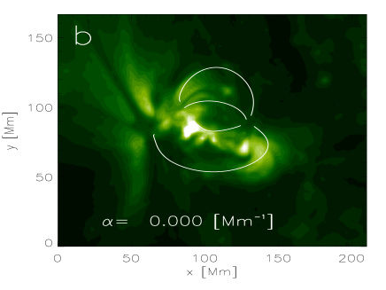
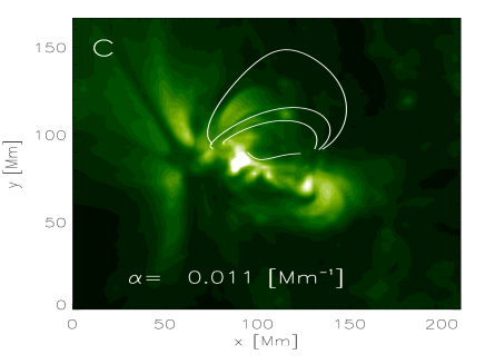
We generalize the method and use the EIT-image (without any pre-identification of structures) together with the fitting routine described in section 2 to compute the optimal value of $\alpha$. To do so, we compute magnetic field lines for several values of $\alpha$ and apply the feature identification method (see Sect. 2) to each of the models and compute the values of $C$ for several loops in each model. As an example we tried to identify coronal loops with the help of a potential field model $\alpha=0$ in Fig. 2 b) and with $\alpha=0.01{\rm Mm}^{-1}$ in Fig. 2 c). It is obvious from the images that the alignment of plasma structures and magnetic field lines is worse than for the optimal value of $\alpha=-0.01{\rm Mm}^{-1}$. The value of $\alpha$ corresponding to the lowest value of $C$ depicts the optimal value of $\alpha$. As a consequence the method automatically computes the optimal coronal magnetic field (within the linear force-free approximation) from LOS-magnetograms and a plasma image (within the limitations listed in Sect. 2.5). In Fig. 2 d) we show quantitatively, with help of the measure define in Eq. 1 how well magnetic field model and emission structures agree with respect to $\alpha$. The minimum of the function depicts the optimal value of the linear force-free parameter, $\alpha=-0.01{\rm Mm}^{-1}$. Let us remark that the main reason for using linear-force free fields are their mathematical simplicity and because non-linear force-free models require vector magnetograms which are often not available or have a limit FOV and high noise/ambiguity in the transversal field. If these data are available a non-linear force-free model is preferred over a linear one. We find, however, that linear force-free fields often give a reasonable approximation of the coronal magnetic field in active regions (much better than potential fields. See section 4 and Wiegelmann et al. (2005)). The linear force-free model has only one free parameter, but in principle one can also use a magnetic field models with several free parameters, e.g. a wider class of magnetohydrostatic equilibria Petrie & Neukirch (2000), together with a multi-dimensional search for the optimal (lowest value of $C$) parameter set.

4 Using different magnetic field models

Figure 3: Identification of loops in H Alpha image with different magnetic field models (a) measured field, (b) linear force-free field with $\alpha=0.085{\rm Mm}^{-1}$, (c) nonlinear force-free field, (d) potential field. We find that all used magnetic field models, except the potential field, identify the loop in the center of the image. The values of $C$ for this loop are a) $1.57$, b) $1.34$, c) $1.34$ and for potential fields almost one order of magnitude worse d) $10.78$. The extrapolated fields (b-c) cannot detect the loop structure in the lower part of the image because of the limited field of view of the vector magnetogram. We applied our identification procedure to the inverse image, because H Alpha is an absorption line.

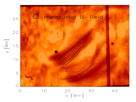
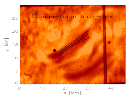
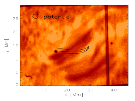
Until now we used linear force-free models for the loop identification and in many cases this will remain the first choice because this model requires only line-of-sight magnetograms, which are routinely observed and available online (MDI: http://soi.stanford.edu/, Kitt Peak: http://www.noao.edu/kpno/). In the near future, when vector magnetograms will be observed routinely (e.g. from SOLIS or Solar-B) non-linear force-free models can be employed.

Here we provide an example of our fitting routine with different magnetic field models. We use a vector magnetogram of the developing active region NOAA 9451 observed with the German Vacuum Tower Telescope (VTT) and the Tenerife Infrared Polarimeter. The pictures have been taken close to the disk center $\mu=cos(\theta)=0.8$ and the images have not been corrected. We compute a potential field and a linear force-free field from the line-of sight component of the magnetogram using the method of Seehafer (1978) (See Figs. 3 b) and d), respectively). With the help of an optimization principle Wheatland, Sturrock, & Roumeliotis (2000); Wiegelmann (2004) we also compute a non-linear force-free field from the full vector magnetogram (See Fig. 3 panel c). For this active region the chromospheric magnetic field vector has been measured Solanki et al. (2003); Lagg et al. (2004) (See Fig. 3 a). The direct field measurements as well as the linear and non-linear extrapolation methods (Fig. 3 panels a-c, respectively) are able to identify a loop structure in the center of a corresponding H Alpha image with similar accuracy $C=1.4^{+}_{-}0.1$. The potential field is not able to identify any structure in the image and the measure $C=10.78$ is almost an order of magnitude higher than for the other magnetic field models. This result is not surprising, because the direct magnetic field measurements have been compared with extrapolated magnetic fields and the comparison revealed that a potential field model was not appropriate for this developing active region Wiegelmann et al. (2005). The comparison with different magnetic field models has revealed that field line parallel electric currents are important to describe the structure and thus the configuration contains magnetic shear.

5 Conclusions and outlook

Within this work we have developed a method for the automatic identification of coronal loops. The method uses a suitable coronal magnetic field model, e.g. from a force-free extrapolation, and compares the projection of 3D magnetic field lines with structures on images, e.g. from SOHO/EIT. As a result coronal structures are represented by 1D curves. A further use of the method is planned in particular for the analysis of data from the two STEREO spacecrafts. The reconstruction of curves is attractive for the STEREO mission for two reasons. Firstly structures on the solar surface are dominated by thin flux tubes which often can well be approximated by idealized curves. Secondly, the stereoscopic reconstruction problem for 1D objects is well posed. Formally, a projected curve in an image can be projected back along the view direction giving rise to a 3D solution surface on which the 3D curve must lie. From two images, we obtain two such surfaces and their intersection must be the solution curve. This is different for a point-like object. Its projection yields two coordinate parameters in two images while only 3 spatial coordinates are required. Formally, the triangulation of point-like objects is therefore over-determined. Conversely, if we want to solve for optically thin, curved surfaces we have an underdetermined problem because the bright limb visible in the two images might project back to different parts of the surface. It is therefore useful to identify 1D objects (loops) out of 2D images for a stereoscopic reconstruction by e.g. tie-point-like methods Hall et al. (2004). Let us remark that the structure identification method by magnetic field lines provides already a 3D structure of the loop which might be further refined by stereoscopic methods. In particular, the advent of the STEREO mission has produced an increased interest of the solar physics community in stereoscopic (Aschwanden et al.,1999,2000 and tomographic techniques Zidowitz (1999); Frazin (2000); Wiegelmann & Inhester (2003) used in other branches of physics, image and information sciences. However, unlike many of the “experiments” conducted in the latter disciplines, the STEREO mission does not provide sufficient control over many of the parameters which determine the conditions for an optimal 3D reconstruction. Tomographic methods will in particular be useful in situations where individual loops cannot be identified due to the superposition of many loops due to the line-of-sight integrated character of 2D images.