Stretching in a model of a turbulent flow
Abstract
Using a multi-scaled, chaotic flow known as the KS model of turbulence [7], we investigate the dependence of Lyapunov exponents on various characteristics of the flow. We show that the KS model yields a power law relation between the Reynolds number and the maximum Lyapunov exponent, which is similar to that for a turbulent flow with the same energy spectrum. Our results show that the Lyapunov exponents are sensitive to the advection of small eddies by large eddies, which can be explained by considering the Lagrangian correlation time of the smallest scales. We also relate the number of stagnation points within a flow to the maximum Lyapunov exponent, and suggest a linear dependence between the two characteristics.
keywords:
PACS:
47. 27. Eq, 47. 52. +j, 47. 27. Gs, and
1 Introduction
Measures of stretching, such as the Lyapunov exponent, are important tools for understanding the nature of dynamical systems. For example, the maximum Lyapunov exponent can provide information about the complexity of an attractor via the Kaplan-Yorke dimension [6], or the rate of loss of information in the system [16]. The use of Lyapunov exponents in turbulent flows is far too great to list here; examples range from probing the onset of turbulence [3], to detecting inhomogeneity in hydromagnetic convection [9]. Another interesting application arises in dynamo theory; it was shown [15] that Lyapunov exponents provide an upper bound for the growth rate of a fast dynamo, and also a non-trivial combination of Lyapunov exponents gives an exact growth rate for the small scale turbulent dynamo [5].
In this work we use a model turbulent flow, known as the Kinematic Simulation (KS) model, that has been primarily used as a Lagrangian model of turbulence [7, 8]. An important feature of KS is that it allows full control of the energy spectrum; moreover, its simple analytic structure means that numerical differentiation is not required in calculating the Lyapunov exponents. The KS model has been shown to be in good agreement with results obtained from direct numerical simulations (DNS) of turbulent flows, particularly with respect to Lagrangian statistics such as two-particle dispersion [8, 10, 11]. The use of the model is spreading rapidly to many other areas such as aeroacoustics and biomechanics. This flow has also been shown to be a hydromagnetic dynamo [17]. Motivated by the success of the KS model and its applications in magnetohydrodynamics, our aim is to check the agreement between the model and turbulent flows with respect to Lyapunov exponents. It has been shown that the KS model exhibits Lagrangian chaos [8, 10]; we shall quantify this feature using the largest Lyapunov exponent.
2 The velocity field
The KS model prescribes the flow velocity at a position and time through the summation of Fourier modes with randomly chosen parameters. These modes are mutually independent, therefore the advection of small eddies by large eddies is not included in the model. More precisely, the velocity field is prescribed to be [11]
| (1) |
where and is the number of modes. The unit vectors are chosen randomly, and where is the wavenumber of the mode. The construction of and , which are time independent, is explained in the appendix. Even though the parameters of the flow are chosen randomly, they do not necessarily change with time, so the flow is not necessarily random. We adopt a normalised energy spectrum of the KS flow , which is a modification of the von Kármán energy spectrum,
| (2) |
which reduces to in the inertial range , with at the integral scale; produces the Kolmogorov spectrum. As mentioned previously, a useful feature of the KS model is the ability to vary the slope in the inertial range. The flow is incompressible and time dependent; the frequency of the mode, is inversely proportional to its turnover time,
| (3) |
It is convenient to write the unit vector as
| (4) |
where, and , are uniformly distributed random numbers, to ensure that are isotropically distributed. With
| (5) |
the effective Reynolds number is introduced using the requirement that the dissipation and eddy turnover times are equal to each other at ,
| (6) |
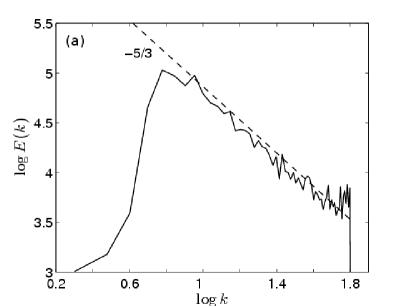
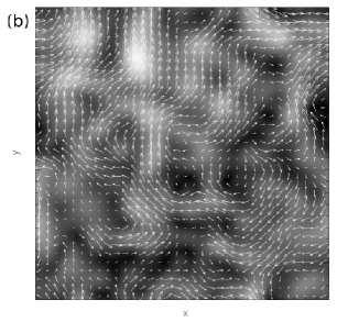
Since the maximum value of and the integral scale remain unchanged in the models discussed here, any variation in Re can be thought to be caused by changes in the fluid viscosity. Fig. 1 shows the energy spectrum of the KS flow, obtained numerically after fast Fourier transforming calculated from Eq. (1) on a mesh. We also show a slice, in the plane, of the corresponding vorticity field, with velocity vectors.
3 The Lyapunov exponents
To obtain the spectrum of Lyapunov exponents, , we measure the average rates of exponential divergence of nearby fluid particle trajectories. If the system is chaotic, at least one Lyapunov exponent is positive. The procedure to calculate the Lyapunov exponents consists of monitoring the evolution of an infinitesimal fluid sphere moving with the flow. The sphere, deformed by the flow, rapidly becomes an ellipsoid. Then the Lyapunov exponents are defined as
| (7) |
where is the ellipsoid’s principal axis, and . Another feature of the KS flow is that it is time reversible (unlike ‘real’ turbulence), therefore the second Lyapunov exponent vanishes [2, 1]. We now consider two remaining exponents, which must have opposite signs, , since the flow is incompressible (), the sum of the Lyapunov exponents must be zero. Hence we only need to calculate one exponent, . Following Wolf et al. [18], consider a sphere whose centre, at , moves along a trajectory defined by
| (8) |
with obtained from Eq. (1). As the sphere follows a trajectory in the flow, its shape is deformed to an ellipsoid by stretching and compression. To the linear approximation in the sphere radius , remains the centre of the deformed ellipsoid. Positions of the points on the surface of the sphere , where is the position of the centre of the ellipsoid, obey the linearised equations of motion
| (9) |
where and the summation convention is assumed. We integrate Eq. (8) and (9) numerically, normalising at regular intervals as to keep the linearisation valid. We then take the temporal average of the magnitude of to recover the maximum Lyapunov exponent. Finally, we average the results over 500 particles to improve statistics. Since detailed behavior of can vary significantly between different realisations of the flow, we further take an ensemble average over 50 different realisations of the KS model with the same non-random parameters. The results of one such run are shown in Fig. 2. Before beginning the simulations, the code was tested by computing Lyapunov exponents for some well known chaotic flows [13].

4 Scaling of the Lyapunov exponent with the Reynolds number
We now determine how scales with the properties of the flow. We begin by considering the relationship between the maximum Lyapunov exponent, , and the Reynolds number, Re. Following Ruelle [12], we increase Re by introducing smaller scales (i.e., increasing ), keeping the same number of modes and the same . In this way we introduce motions with higher velocity shear rate. The maximum Lyapunov exponent is the modulus of the long-term average of the velocity gradient in the Lagrangian frame. In fully developed turbulence this is related to the turnover time of the smallest eddies, where the turnover time of an eddy of size is
| (10) |
where is the integral scale, the corresponding velocity (with ) and the Hölder exponent of the velocity field, introduced as
| (11) |
Then scales with Re as
| (12) |
where and is the Kolmogorov length scale. For the Kolmogorov spectrum, , we have and .
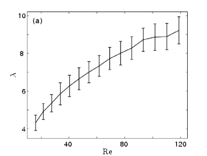
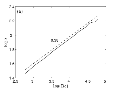
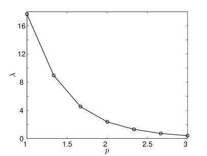
Our numerical simulations, illustrated in Fig.3, show that the largest Lyapunov exponent of the KS model scales as , thus is smaller than Ruelle’s prediction. This difference may arise from the lack of sweeping of the small eddies by the large eddies in the KS model. In KS, like in real turbulence, velocity is determined by the large scale ‘eddies’, and velocity gradients are determined by the small scale motions. But, the Lyapunov exponent is related to velocity gradients in the Lagrangian frame, hence the lack of advection of the small eddies is important. Because of the lack of advection, the Lagrangian correlation time of eddies of size is , not . The maximum Lyapunov exponent is related to this correlation time, hence there is a reduction in the expected value of , that grows with Re. We are grateful to an anonymous referee who suggested this explanation.
Hence we must be careful when applying the KS model to area’s where stretching is important, especially if we are comparing results with DNS, and scaling with Re. Dynamo action is one of such areas.
5 Lyapunov exponents, spectral slope and stagnation points
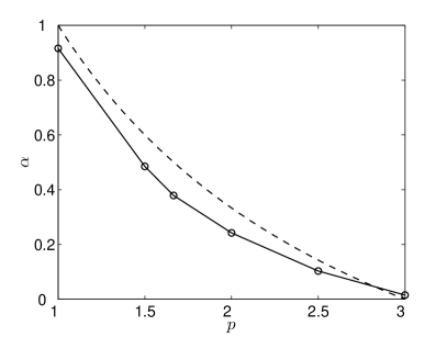
Since the shear rate increases with the wave number for a sufficiently steep spectrum, the main cause of stretching are the small scale motions, described well by the KS model. Therefore, we should not be too worried about the discrepancy described at the end of the previous section. Of our primary interest here (motivated by the saturation of the fluctuation dynamo) is the effect of the slope of the energy spectrum plays on stretching. Cattaneo et al. [4] showed, using a simple chaotic velocity field, that as a dynamo saturates, Lagrangian chaos in the flow is suppressed. With a complex multi-scaled flow such as turbulence this effect would remove energy from small scales first, stimulating us to study the effect of steepening the spectrum on . To study how depends on , we fix and and change the spectral slope in Eq. (2). The resulting values of , shown in Fig. 4, have been obtained by averaging over particles in the same flow. These results confirm that the largest Lyapunov exponent is controlled mainly by the smaller scales: as less energy is given to the small scales, decreases. The next logical step is to investigate the effect of on the scaling parameter . Indeed, in Eq. (11) and then
| (13) |
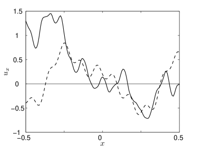
from Eq. (12). This dependence is shown dashed in Fig. 5 along with the results from our simulations. As before, our estimates of are smaller, but we expect this due to the absence of sweeping. If KS is to be used in areas sensitive to stretching, we suggest the inclusion of the advection of small eddies [7]. We would then expect the value of to be closer to Ruelle’s prediction. It can be expected that the velocity shear rate, and hence the amount of stretching, is maximum near stagnation points where velocity changes most rapidly in space. The number of stagnation points per unit volume (and hence the total magnitude of velocity shear) is sensitive to the number of modes in the KS model. The smaller is the value of for large , the more numerous will be the stagnation points [14], see Fig. 6. Although our velocity field is time-dependent, it has infinite correlation time, so that the density of stagnation points varies little in time. We computed the maximum Lyapunov exponent for fixed and , but with an increasing number of modes, .
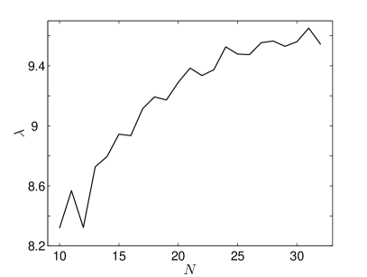
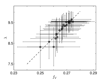
Since the number of stagnation points in the flow increases with , we expect that increases too. Fig. 7 confirms this and also shows that saturates as grows. The abundance of stagnation points in the flow can be quantified using what we call the volume filling factor calculated as
| (14) |
where the summation is extended over all the mesh points in the computational box, is the number of mesh points along each direction, is the root-mean-square velocity, and is the Heaviside function,
| (15) |
Thus defined, this the fractional volume of the region where . We calculated in a KS flow with modes with in a box whose size is , the largest scale in the flow, and we average over 500 realisations of the flow. Fig. 8 shows a scatter plot of versus for an increasing number of modes in the model. Despite the large error bars, the data suggests a linear relationship. The magnitude of the errors may be due to the variation between different realisations of the flow.
6 Conclusions
Our simulations confirm that the KS model reproduces reasonably well the stretching properties of turbulent flows, including the scaling of the maximum Lyapunov exponent with the Reynolds number despite the fact that the latter can only be introduced formally in the KS model. The model values of the Lyapunov exponent are always smaller than theoretical predictions for turbulent flows; we attribute this to the lack of advection of the small eddies by the large eddies in the model. Hence we must be careful when applying the KS model to area’s where stretching is important. Finally our results suggest a linear relationship between the number of stagnation points in the flow and .
Appendix A Appendix
We choose , and randomly, imposing orthogonality with , which gives the required spectrum as
| (16) |
we proceed in the same fashion for . We then choose
| (17) |
This ensures
| (18) |
where is given by
| (19) |
References
- [1] J. Bec, L. Biferale, G. Boffetta, M. Cencini, S. Musacchio, F. Toschi, Lyapunov exponents of heavy particles in turbulence, Physics of Fluids 18 (9) (2006) 091702.
- [2] G. Benettin, L. Galgani, J.-M. Strelcyn, Kolmogorov entropy and numerical experiments, Phys. Rev. A 14 (6) (1976) 2338–2345.
- [3] A. Brandstater, H. L. Swinney, Strange attractors in weakly turbulent couette-taylor flow, Phys. Rev. A 35 (1987) 2207–2220.
- [4] F. Cattaneo, D. W. Hughes, E. Kim, Suppression of chaos in a simplified nonlinear dynamo model, Phys. Rev. Lett. 76 (1996) 2057–2060.
- [5] M. Chertkov, G. Falkovich, I. Kolokolov, M. Vergassola, Small-scale turbulent dynamo, Phys. Rev. Lett. 83 (20) (1999) 4065–4068.
- [6] H. Froehling, J. P. Crutchfield, D. Farmer, N. H. Packard, R. Shaw, On determining the dimension of chaotic flows, Physica D 3 (1981) 605–617.
- [7] J. C. H. Fung, J. C. R. Hunt, A. Malik, R. J. Perkins, Kinematic simulation of homogeneous turbulence by unsteady random fourier modes, J. Fluid Mech. 236 (1992) 281–318.
- [8] J. C. H. Fung, J. C. Vassilicos, Two-particle dispersion in turbulent-like flows, Phys. Rev. E 57 (1998) 1677–1690.
- [9] J. Kurths, A. Brandenburg, Lyapunov exponents for hydromagnetic convection, Phys. Rev. A 44 (1991) R3427–R3429.
- [10] A. Malik, J. Vassilicos, A lagrangian model for turbulent dispersion with turbulent-like flow structure: Comparison with direct numerical simulations for two particle statistics, Phys. Fluids 11 (1999) 1572–1580.
- [11] D. Osborne, J. Vassilicos, K. Sung, J. Haigh, Fundamentals of pair diffusion in kinematic simulations of turbulence, Phys. Rev. E 74 (2006) 036309.
- [12] D. Ruelle, Microscopic fluctuations and turbulence, Phys. Lett. A 72 (1979) 81–83.
- [13] J. C. Sprott, Chaos and Time-Series Analysis, Oxford University Press, 2003.
- [14] J. C. Vassilicos, private communication (2007).
- [15] M. M. Vishik, Magnetic field generation by the motion of a highly conducting fluid, Geophys. Astrophys. Fluid Dyn. 48 (1989) 151–161.
- [16] D. J. Wales, Calculating the rate of loss of information from chaotic time series by forecasting, Nature 350 (1991) 485–488.
- [17] S. L. Wilkin, C. F. Barenghi, A. Shukurov, Magnetic structures produced by the fluctuation dynamo, Phys. Rev. Lett. 99 (2007) 134501–134505.
- [18] A. Wolf, J. B. Swift, H. L. Swinney, J. A. Vastano, Determining lyapunov exponents from a time series, Physica D 16 (1985) 285–317.