Entanglement dynamics and relaxation in a few qubit system interacting with random collisions

Abstract

The dynamics of a single qubit interacting by a sequence of pairwise collisions with an environment consisting of just two more qubits is analyzed. Each collision is modeled in terms of a random unitary operator with a uniform probability distribution described by the uniform Haar measure. We show that the purity of the system qubit as well as the bipartite and the tripartite entanglement reach time averaged equilibrium values characterized by large instantaneous fluctuations. These equilibrium values are independent of the order of collision among the qubits. The relaxation to equilibrium is analyzed also in terms of an ensemble average of random collision histories. Such average allows for a quantitative evaluation and interpretation of the decay constants. Furthermore a dependence of the transient dynamics on the initial degree of entanglement between the environment qubits is shown to exist. Finally the statistical properties of bipartite and tripartite entanglement are analyzed.

1 Introduction

The repeated collision model has been recently used in literature to analyze the irreversible dynamics of a qubit interacting with a reservoir consisting of a large number of environmental qubits. In particular processes like thermalization [1] and homogenization [2, 3, 4, 5], have been analytically investigated. The same model has ben used recently also to analyze the dynamics of a qubit interacting with a very small environment consisting of just two qubits [6]. The interest for such system is due to the fact that, at variance with what happens in the case of an environment with a large number of degrees of freedom, the system dynamics cannot be described by a Markovian master equation. Indeed, due to the fact that the system qubit collides repeatedly with the same environment qubits, the dynamics is characterized by large fluctuations and only when the sequence of collision is random a time averaged equilibrium is reached. While in all the above mentioned papers the - elastic - collisions have been modeled by a partial swap unitary operator, in the present paper we will analyze the system dynamics in the case in which the two-qubit collisions are described by random unitary operators [7, 8, 9, 10, 11, 12].

Random unitary operators have received considerable attention in quantum information theory, mainly because they find applications in various quantum protocols [13, 14, 15, 16]. Unfortunately the implementation of a random unitary operator acting on the $n$-qubit Hilbert space requires a number of elementary quantum gates that is exponential in the number of qubits. On the other hand sequences of random two-qubit gates (collisions) generate pseudo-random unitary operators which approximate, to the desired accuracy, the entanglement properties of true $n$-qubit random states [17, 18, 19, 20, 21, 22, 23]. This approach has given very good results, showing that pseudo-random states can be generated efficiently, that is polynomially in $n$ [17, 18, 19, 20, 21, 22, 23].

Our choice to describe the pairwise collisions in terms of random two qubit unitary operators is motivated by the fact that often a precise modelization of the interaction is very hard and that, on the other hand, a good description of the approach to equilibrium can be obtained by suitable averages of the quantities of interest, as we will describe below. Furthermore such collision model exhibits interesting features ranging from memory effects to the efficient entanglement generation between system and environment.

2 The model

In order to illustrate the approach of our work, we first review the repeated collision model. Let us consider a set of $N+1$ qubits, the first of which is the system qubit and the remaining $N$ are the reservoir. The system-environment interaction is due to pairwise collisions between the system and a singe reservoir qubit. After $t$ collisions the overall state of the system plus reservoir is

$$\varrho_{SE}^{(t)}=U_{i_{t}}\cdots U_{i_{2}}U_{i_{1}}\varrho_{SE}^{(0)}U_{i_{1}}^{\dagger}U_{i_{2}}^{\dagger}\cdots U_{i_{t}}^{\dagger},$$ (1)

where $\varrho_{SE}$ is the total density operator and the sequence $i_{1}\cdots i_{t}$ specify the order with which the environment qubits collide with the system one. As in [6] we have concentrated our attention to the case in which the environment consists of just two qubits. In the following $0$ will label the system qubit while $1,2$ will label the environment qubits. At variance with the previous work, however, we have considered here the case in which each collision is described by a random unitary operator $U_{i}$ picked up from the uniform Haar measure on the group $U(4)$. In particular in our calculations we have found convenient to parametrize each random unitary matrix $U_{i}$, in terms of the Hurwitz representation of the unitary group $U(4)$ [26, 12, 20]. Such different choice of the collision unitary operators has several consequences. First of all the collisions are of course no longer elastic and, regardless of the number of environment qubits, homogenization is no longer achieved. However, even for a few qubits environment, a time averaged equilibrium state with large fluctuations is reached regardless of the order with which the qubits collide (in the numerical data shown below, we consider random sequences $i_{1},\cdots i_{t}$). Furthermore such equilibrium state is independent of the initial state of the qubits. In the following we will characterize some aspects of such approach to a time averaged equilibrium state.

Random qubit-environment interactions have been recently considered [24, 25], for high dimensional environments. However in our work we deal with small environments, such that the information acquired by the environment on the system can flow back to the system and a Markovian description of our model is surely not possible. Moreover, there is no weak coupling parameter and the state of the environment is significantly affected by the interaction at each collision, so that also the Born approximation does not apply.

3 Approach to equilibrium

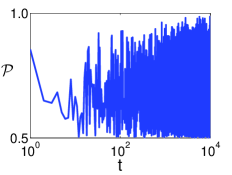
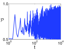
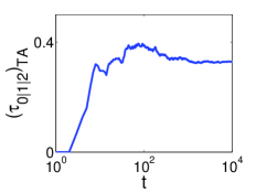
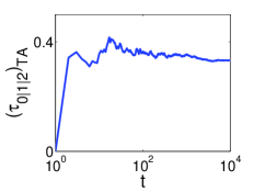
We have characterized the decoherence of the system qubit in terms of the purity $\mathcal{P}$. We remind the reader that the purity is defined as $\mathcal{P}=\hbox{Tr}\left[{\varrho_{S}^{2}}\right]$, where $\varrho_{S}=\hbox{Tr}_{E}\left[\varrho_{SE}\right]$ is the reduced density operator of the system qubit. The purity is a decreasing function of the degree of statistical mixture of the qubit and takes values in the range $\frac{1}{2}\leq\mathcal{P}\leq 1$ where $\mathcal{P}=1$ corresponds to pure states and $\mathcal{P}=\frac{1}{2}$ to the completely unpolarized mixed state. As already mentioned, due to the small number of environment qubits, the instantaneous system purity undergoes large fluctuations regardless of the initial state of both the system and the environment and regardless of the sequence of collisions as shown in Fig. 1 (first row). The purity, however, approaches a time averaged equilibrium state. To see this we calculate the time averaged purity $\mathcal{P}_{TA}(t)$ as

$$\mathcal{P}_{TA}(t)=\frac{1}{t+1}\sum_{t^{\prime}=0}^{t}\hbox{Tr}\left[\rho_{S}^{2}(t^{\prime})\right].$$ (2)

As shown in Fig. 1 (second row), $\mathcal{P}_{TA}(t)$ reaches the same equilibrium value regardless of the initial entanglement of the environment qubits, a natural consequence of the random nature of the collisions.

Figure 1: From top to bottom: instantaneous, time averaged and ensemble averaged purity, for an environment in an initial product (left) or maximally entangled (right) state. The time evolution of the ensemble averaged purity is in both cases well fitted by the exponential curve $\mathcal{P}_{EA}(t)-\mathcal{P}_{L}\propto\exp(-0.36t)$, with $\mathcal{P}_{L}=\frac{2}{3}$ (asymptotic horizontal line).

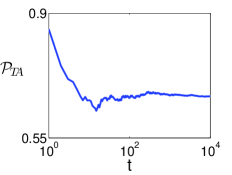
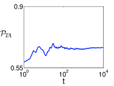
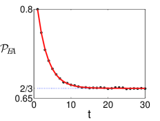
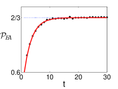
Further insight into the approach to equilibrium of the system qubit is obtained if rather than the time average purity we evaluate the ensemble averaged purity $\mathcal{P}_{EA}(t)$ over the uniform Haar measure. As we shall see, an analysis of the time evolution of such averaged quantity allows us to determine the time scale for the relaxation to equilibrium. To evaluate $\mathcal{P}_{EA}(t)$ we have generated a large number of sequences of random collisions, each one drawn from the uniform measure, and we have averaged the purity over the different histories after $t$ steps. Also such ensemble average shows an irreversible behaviour of the qubit dynamics. Regardless of the initial state of the environment qubits, $\mathcal{P}_{EA}(t)$ decays to the value $\frac{2}{3}$, which coincides with the average purity $\mathcal{P}_{L}$ predicted by Lubkin [28] for true overall (system-environment) random states. Note that $\mathcal{P}_{TA}(t)$ and $\mathcal{P}_{EA}(t)$ tend to the same asymptotic value. If $\mu$ and $\nu$ are respectively the dimensions of the Hilbert space of the system and of the environment one has

$$\mathcal{P}_{L}=\frac{\mu+\nu}{\mu\nu+1}.$$ (3)

In our case $\mu=2$ and $\nu=4$, and therefore $\mathcal{P}_{L}=\frac{2}{3}$. However, as shown in Fig. 1 (third row) the time evolution of $\mathcal{P}_{EA}(t)$ exhibits a clear dependence on the degree of entanglement of the initial state of the environment qubits. Notably the exponential approach to equilibrium is for the first collisions a decreasing (increasing) function of $t$ for an environment in an initial product (maximally entangled) state. In both cases a numerical fit shows that $\mathcal{P}_{EA}(t)-\mathcal{P}_{L}\propto\exp(-\lambda t)$ with $\lambda\approx 0.36$.

The asymptotic relaxation to equilibrium can be computed analytically following the approach developed in [21, 22, 23]. Each pure three-qubit state $\rho_{SE}$ can be expanded over products of Pauli matrices: $\rho_{SE}=\sum_{\alpha_{0},\alpha_{1},\alpha_{2}}c_{\alpha_{0}\alpha_{1}\alpha_{2}}\sigma_{0}^{\alpha_{0}}\otimes\sigma_{1}^{\alpha_{1}}\otimes\sigma_{2}^{\alpha_{2}}$, where $\sigma_{i}^{\alpha_{i}}$ denotes a Pauli matrix acting on the $i$th qubit, with $\alpha_{i}\in\{0,x,y,z\}$ and $\sigma^{0}=I$. The purity then reads $\mathcal{P}(t)=\sum_{\alpha_{0}}c_{\alpha_{0}00}^{2}(t)$. The purity decay can therefore be obtained from the evolution in time of the coefficients $c_{\alpha_{0}00}^{2}$. For the random collision model the column vector $c^{2}$ of the coefficients $c_{\alpha_{0}\alpha_{1}\alpha_{2}}^{2}$ evolves according to a Markov chain dynamics of the form $c^{2}(t+1)=Mc^{2}(t)$ [23]. The matrix $M$ is obtained after averaging over the two possible couplings $01$ and $02$: $M=\frac{1}{2}(M^{(2)}_{01}+M^{(2)}_{02})$, with $M^{(2)}_{ij}$ acting non trivially (differently from identity) only on the subspace spanned by qubits $i$ and $j$. Averaging over the uniform Haar measure on $U(4)$ one can see that $M^{(2)}_{ij}$ preserves identity ($\sigma_{i}^{0}\otimes\sigma_{j}^{0}\to\sigma_{i}^{0}\otimes\sigma_{j}^{0}$) and uniformly mixes the other $15$ products $\sigma_{i}^{\alpha_{i}}\otimes\sigma_{j}^{\alpha_{j}}$ [23]. The matrix $M$ has an eigenvalue equal to $1$ (with multiplicity $2$) and all the other eigenvalues smaller than $1$. Therefore the asymptotic purity decay is determined by the gap $\Delta$ in the Markov chain, namely by the second largest eigenvalue $1-\Delta$ of the matrix $M$. We have $\mathcal{P}_{EA}(t)-\mathcal{P}_{L}\asymp(1-\Delta)^{t}=\exp\{[\ln(1-\Delta)]t\}$. In our model $1-\Delta=0.7$ (eigenvalue with multiplicity $2$) and therefore $-\ln(1-\Delta)\approx 0.357$, in very good agreement with the value $\lambda\approx 0.36$ obtained from our fit.

4 Entanglement dynamics

The dynamics of bipartite and multipartite entanglement between the qubits of our model shows interesting features. Such dynamics has been conveniently characterized in terms of the concurrence and of the tangles [30, 31]. We remind the reader that, given the density operator $\rho_{ij}$ of a bipartite system of two qubits, the tangle $\tau_{i|j}$ is defined as

$$\tau_{i|j}(\rho)=[\max\left\{0,\alpha_{1}-\alpha_{2}-{\alpha_{3}}-{\alpha_{4}}\right\}]^{2},$$ (4)

where $\left\{\alpha_{k}\right\}$ ($k=1,..,4$) are the square roots of the eigenvalues (in non-increasing order) of the non-Hermitian operator $\bar{\rho}_{ij}=\rho_{ij}(\sigma_{y}\otimes\sigma_{y})\rho_{ij}^{*}(\sigma_{y}\otimes\sigma_{y})$, $\sigma_{y}$ is the $y$-Pauli operator and $\rho_{ij}^{*}$ is the complex conjugate of $\rho_{ij}$, in the eigenbasis of the $\sigma_{z}\otimes\sigma_{z}$ operator. The concurrence $C$ is defined simply as $C_{ij}=\sqrt{\tau_{i|j}}$. The tangle $\tau_{i|j}$, or equivalently the concurrence $C_{ij}$ can be used to quantify the entanglement between the pair of qubits $i,j$ for an arbitrary reduced density operator $\rho_{ij}$. Furthermore, when the overall state of the system is pure, the amount of entanglement between qubit $i$ and all the remaining can be quantified by the tangle $\tau_{i|\mbox{rest}}=4\det\rho_{i}$. The tangle $\tau_{0|\mbox{rest}}$ between the system qubit and the environment conveys the same information as the purity $\mathcal{P}$. Indeed it is easy to show that $\tau_{0|\mbox{rest}}=2-2{\mathcal{P}}$. We have numerically computed the tangles $\tau_{0|1}$, $\tau_{0|2}$, and $\tau_{1|2}$ of the two-qubit reduced density matrices and the three-tangle $\tau_{i|j|k}=\tau_{i|jk}-\tau_{i|j}-\tau_{i|k}$, where $i,j,k$ can be any permutation of $0,1,2$ and where the tangle $\tau_{i|jk}$ measures the entanglement between the $i$th qubit and the rest of the system, i.e., qubits $j,k$. The three-tangle $\tau_{0|1|2}$ is a measure of the purely tripartite entanglement and is invariant under permutations of the three qubits [31].

The instantaneous dynamics of the tangles $\tau_{i|j}$ and of the three-tangle $\tau_{0|1|2}$ is similar to the dynamics shown in the Fig. 1 (top) for the purity, that is, these quantities are characterized by large instantaneous fluctuations. However the time averaged tangles $(\tau_{i|j})_{TA}(t)$, defined in analogy with Eq.(2), approach the same limiting value $\tau_{P}$.

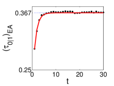
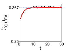
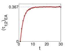
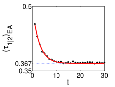
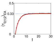
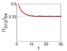
Again we have numerically evaluated the ensemble average (with respect to the Haar measure) tangles $(\tau_{i|j})_{EA}(t)$. As shown in Fig. 2 (bottom) the pairwise tangles $(\tau_{0|1})_{EA}(t)$ and $(\tau_{0|2})_{EA}(t)$ approach exponentially the same equilibrium value $\tau_{P}\approx 0.367$. The numerical data in Fig. 2 (bottom) are well fitted by the curves $(\tau_{i|j})_{EA}(t)-\tau_{P}\propto\exp(-\lambda_{ij}t)$. When the environment is initially separable we obtain $\lambda_{01}\approx\lambda_{02}\approx 0.76$, $\lambda_{12}\approx 0.44$, while for an initially maximally entangled states of the environment we have $\lambda_{01}\approx\lambda_{02}\approx 0.44$, $\lambda_{12}\approx 0.36$. Therefore, initially entangled environment qubits limit the rate of generation of bipartite entanglement between the qubit system and a single environment qubit, even though the amount of pairwise entanglement obtained asymptotically is always the same. We have furthermore verified also that the average tangle $(\tau_{1|2})_{EA}$ approaches the same limiting value $\tau_{P}$ even though the environment qubits do not collide directly.

Figure 2: Time (first row) and ensemble (second and third rows) averages for the pairwise tangles $\tau_{0|1}$ (solid line in the first row), $\tau_{0|2}$ (dashed line in the first row) and $\tau_{1|2}$ (dotted line in the first row), for an environment in an initial product (left) or maximally entangled (right) state. For the ensemble averaged quantities also the fit $(\tau_{i|j})_{EA}(t)-\tau_{P}\propto\exp(-\lambda_{ij}t)$ is shown. In the second row only the $(\tau_{0|1})_{EA}(t)$ is shown due to the same figure of $(\tau_{0|2})_{EA}(t)$

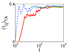
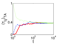
As one would expect from the above discussion, also the mutipartite entanglement approaches an equilibrium value. This can be seen by the time and ensemble averages three-tangle $\tau_{0|1|2}$ shown in Fig. 3. The approach to the equilibrium value $\tau_{T}$ is exponential also for this quantity and we can extract the convergence rate from the fit $(\tau_{0|1|2})_{EA}(t)-\tau_{T}\propto\exp(-\lambda_{012}t)$, with $\lambda_{012}=0.36$ regardless on whether the initial state of the environment is entangled or separable.

Figure 3: Time (top) and ensemble (bottom) averages for the three-tangle $\tau_{0|1|2}$ for an environment in an initial product (left) or maximally entangled (right) state. For the ensemble averaged quantities also the fit $(\tau_{0|1|2})_{EA}(t)-\tau_{T}\propto\exp(-0.36t)$ is shown.

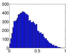
Finally, we note that not only the time and ensemble averages of the various tangles converge to the same limit values regardless of the initial conditions, but also to a well defined limit distribution. In particular the concurrences are distributed in accordance with the distribution shown in in Fig.3 of [27] for random pure $3$-qubit states. Finally the numerically calculated distributions of the three-tangle in our collision model are shown in Fig. 4, for separable and for entangled initial environment state.

Figure 4: Statistical distributions of the three-tangle $\tau_{0|1|2}$, for separable (left) and entangled (right) initial state of the environment. In both cases $\tau_{0|1|2}=0.33\pm 0.19$.

5 Conclusions

In summary, we have shown that relaxation (in time average) to statistical equilibrium is possible for a system of just three qubits undergoing purely random unitary evolution, regardless of the order of the collisions (in contrast to the case studied in [6]). This process is intrinsically irreversible (in contrast to [1, 2]) due to the random nature of the interactions. The purity of the qubit system shows an exponential decay and the decay rate has been evaluated both numerically and analytically. The limit value is in accordance with [28]. The limit values (in a time average sense) of the pairwise qubit tangles are the same for all possible qubit pairs. In contrast to [6], residual entanglement (three-tangle) is generated regardless of initial entanglement of the environment qubits.