Dynamics of gene expression and the regulatory inference problem

Abstract

From the response to external stimuli to cell division and death, the dynamics of living cells is based on the expression of specific genes at specific times. The decision when to express a gene is implemented by the binding and unbinding of transcription factor molecules to regulatory DNA. Here, we construct stochastic models of gene expression dynamics and test them on experimental time-series data of messenger-RNA concentrations. The models are used to infer biophysical parameters of gene transcription, including the statistics of transcription factor-DNA binding and the target genes controlled by a given transcription factor.

1 Introduction

The primary step in the production of a protein is the transcription of a gene from the DNA template to a m(essenger)-RNA molecule. Gene transcription is carefully controlled, allowing the cell to respond to situations requiring different proteins: for instance, enzymes are produced when nutrients need to be processed and repair proteins are assembled to respond to cell damage.

The cellular information processing to achieve this control has a concrete biophysical basis. Transcription factor molecules locate and bind to specific sites on DNA found in the regulatory region in front of a gene. The transcription factors then attract or repel the molecular machinery that reads off the gene (see Fig. 1(a)). The resulting gene product may itself be a transcription factor, enhancing or suppressing the transcription of further genes. The dynamics of gene expression is thus governed by a complex web of molecular interactions. Changes in the regulatory interactions (caused for instance by mutations in a transcription factor binding site) disrupt the cellular dynamics and can lead to serious defects, including cancer.

Which transcription factor targets which gene can in principle be determined experimentally, by investigating the physical binding of transcription factors to the regulatory DNA of a target gene. High-throughput methods have resulted in lists of potential target genes for many transcription factors [1, 2], which, however, contain many false positives and false negative results. Binding sites for transcription factors can also be identified computationally by searching regulatory DNA for statistically overrepresented subsequences [3, 4].

Both approaches, however, tell nothing about the function of a transcription factor (for instance its activity as an inhibitor or an enhancer of gene transcription), or about its interplay with other transcription factors. Moreover, some transcription factors (called co-factors) do not bind directly to DNA but to other transcription factors, and thus do not have binding sites on DNA. As a result, even in well-studied organisms such as yeast, the function and target genes of about half the transcription factors remain unknown [5].

(a)

(b)

Figure 1: Biophysics of gene transcription and its experimental measurement. a) Transcription factors are proteins which bind to specific sites on DNA. These binding sites are located in the so-called regulatory region of a gene, which for yeast typically extends over several hundred nucleotides before the starting point of transcription (marked with the arrow). A fully assembled set of transcription factors will attract and activate the machinery (called RNA-polymerase) which transcribes the DNA template to an mRNA molecule. In a further step, the mRNA molecule will be translated to a protein.
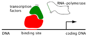
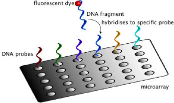
b) DNA-microarrays can simultaneously measure mRNA expression levels in a sample for all genes of an organism. A sample is taken from a population of cells in a certain state, so even for low expression levels of a gene, the number of molecules is macroscopic. (Single-cell fluctuations are averaged out in this process.) mRNA in a sample is reversely transcribed to DNA and deposited on a chip, which has a strand of complementary DNA grafted onto its surface. The DNA in the sample will bind to its complement on the chip. Fluorescent labelling of the DNA in the sample allows to determine the original mRNA concentration relative to a reference sample. By photolithographic techniques, hundreds of thousands of such DNA-probes can be placed on a single microarray-chip. By now over $10^{5}$ genome-wide experimental measurements of mRNA-expression levels have been performed for different organisms, under different experimental conditions, or for different tissues [6].

The development of microarrays has made it possible to simultaneously measure the expression levels (mRNA concentrations) of all genes of an organism (see Fig. 1(b)). This allows to probe the response of the regulatory network to external perturbations, or to detect correlations of expression levels of different genes [7].

The effort to deduce the input-output relations of regulatory networks from experimental gene expression data, however, is impeded by the large number of such relations which are compatible with a given set of expression levels [8]. For instance, an observed correlation between mRNA concentration of two genes may stem from a causal relationship (one gene regulates the expression of the other), or from both genes sharing a common regulator [7]. As a result, many machine learning approaches to the network reconstruction problem, such as Bayesian probabilistic models (see [9, 10] for reviews), or linear regression [11] are well-known to be afflicted with the curse of dimensionality [8, 12].

Here we take a biophysics approach to gene transcription. The inference of the biophysical machinery underlying gene transcription from its output is a challenging inverse problem akin to unravelling the principles of atomic physics from spectroscopy or the events in the early universe from cosmic radiation. In this paper, the statistics of gene expression dynamics is deduced from experimental data. Based on this statistics, a Langevin model for the non-equilibrium dynamics of mRNA concentrations is used to infer basic biophysical parameters of expression dynamics, including mRNA degradation constants, the statistics of transcription factor-DNA interactions, and regulatory interactions.

2 Modelling gene expression dynamics

The basic processes driving the concentration of mRNA are transcription, which creates mRNA molecules at a certain rate, and mRNA degradation, which destroys molecules at a rate proportional to their abundance. This dynamics gives rise to the well-known linear equation of motion [13, 14] for the concentration $x$ of mRNA of a given gene

$$\partial_{t}x=-\eta x+f\ ,$$ (1)

where $\eta$ is a mRNA-specific degradation constant and $f$ is the transcription rate.

To model changes in the transcription rate over time, this deterministic dynamics is generalized to a stochastic process described by [15, 16, 17]

$$\partial_{t}x\equiv\frac{x(t+\Delta_{t})-x(t)}{\Delta_{t}}=-\eta x+f+\sqrt{D/\Delta_{t}}\,\xi(t)\ .$$ (2)

At this point, the term $\xi(t)$ describes lack of knowledge regarding regulation by gene-specific transcription factors whose concentrations vary over time, and possible experimental noise. We model this term by a random variable, whose mean and variance are zero and one, respectively, without loss of generality. Regulation will be incorporated below. The amplitude $\sqrt{D/\Delta_{t}}$ of this noise term is characterized by a ‘diffusion constant’ $D$ and the interval $\Delta_{t}$ between two successive measurements. Equation (2) is well-known as the Langevin equation describing an Ornstein-Uhlenbeck process [18].

The soundness of (2) as a model of mRNA dynamics can be probed by separating deterministic and stochastic contributions to the dynamics. The drift term $\langle(x_{t+1}-x_{t})/\Delta_{t}\rangle$ is computed by considering all instances of concentration $x_{t}=x$ in a time course. We use the time course data by Spellman et al. [19], where expression levels of all yeast genes were measured at intervals ranging from $7$ to $20$ minutes, see Appendix. The expression ratios (fluorescence measured relative to a reference sample, also termed expression levels) were used as measures of mRNA concentration. This is valid provided the fluorescence/concentration response is in the linear regime [20]. The result for a specific mRNA shown in Fig. 2(a) is compatible with the linear relationship $\langle\partial_{t}x\rangle=-\eta x+f$. Genome-wide results will be discussed below. Similarly, the distribution of the noise $\xi(t)$ can be deduced from the data, This distribution is shown for a single gene in Fig. 2(b) and is found to be compatible with a Gaussian distribution. A Kolmogorov-Smirnov test shows that this holds also for all other genes.

(a)

(b)

(c)

(d)

(e)

(f)

Figure 2: Statistics of mRNA concentration dynamics: Drift and diffusion. a) The average rate of expression level change, or drift $\langle(x_{t+1}-x_{t})/\Delta_{t}\rangle$ for a single mRNA species is plotted against the expression levels $x_{t}$, by binning a time course of $35$ measurements into $5$ bins. The mRNA chosen for this example is encoded by gene YN40, which probably codes for a cell wall protein [21]. b) Solving (2) for $\xi(t)$, the statistics of the stochastic term can be estimated, shown here for the example gene YN40. c) To allow comparison of genes with different decay constants and transcription rates, rescaled expression values $q$ were used to compute the drift of $q$ for all genes in yeast, see text. The genome-wide result agrees well with the linear decay law $\langle\partial_{t}q/\eta\rangle=-q$ indicated by the solid line. d) The genome-wide distribution of the noise term $P(\xi)$, see text. e) The standard deviation $\sigma_{\xi}(q)$ of the noise term is shown against the rescaled expression level $q$. f) The distribution $P(\xi_{t},\xi_{t+\Delta})$ of noise terms at subsequent time intervals $t$ and $t+\Delta$, see text.

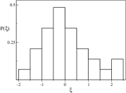
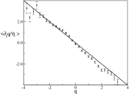
For a Gaussian noise statistics, the equation of motion (2) gives the conditional probability of going from concentration $x_{t}$ to $x_{t+1}$ in a given short time step as

$$G_{\eta,f,D}(x_{t+1}|x_{t})$$

$$= \frac{1}{\sqrt{2\pi D\Delta_{t}}}\exp{\left\{-\frac{\Delta_{t}}{2D}(\partial_{t}x+\eta x_{t}-f)^{2}\right\}}\ .$$

Assuming uncorrelated noise, the propagator (2) gives the probability for a complete time course of mRNA expression levels, ${\bf x}=(x_{1},x_{2},\ldots,x_{T})$, starting from some initial point $x_{1}$, as

$${\mathcal{P}}_{\eta,f,D}({\bf x})=\prod_{t=1}^{T-1}G_{\eta,f,D}(x_{t+1}|x_{t})\ .$$ (4)

In order to determine the model parameters we now ask which parameter values $\eta,f,D$ give the highest likelihood (4) to a given time course ${\bf x}$. This leads to the straightforward maximum likelihood estimates [22]

$$(\eta^{\star},f^{\star},D^{\star})={\arg\!\max}_{\eta,f,D}{\mathcal{P}}_{\eta,f,D}({\bf x})\ .$$ (5)

The time intervals $\Delta_{t}$ between adjacent time points frequently differ from one another. This makes parameters estimates from (2) – (5) distinct from fitting data to a deterministic model with a quadratic penalty of residuals [23, 24, 25].

The experimental data [19] gives expression level time courses for nearly all $\sim 6000$ yeast genes. This allows to probe the model (2) on a genome-wide scale with high statistical accuracy. In order to compare the dynamics of genes with different values of the parameters $\eta,f,D$ we introduce rescaled expression levels $q=\sqrt{2/(D\eta)}(\eta x-f)$ so the Langevin equation (2) reads $\partial_{t}q=-\eta q+\sqrt{2\eta/\Delta_{t}}\xi(t)$ and distribution of $q$ in equilibrium is independent of the parameters, $P(q)\sim\exp\{-q^{2}/2\}$.

The average rate of change (drift) of rescaled expression levels $q$ between two successive time steps is shown in Fig. 2(c) for all genes. The linear relationship $\langle\partial_{t}q/\eta\rangle=-q$ is obeyed quite accurately. Similarly, the distribution of the noise term $\xi(t)$ across all genes, shown in Fig. 2(d), rather closely follows a Gaussian distribution.

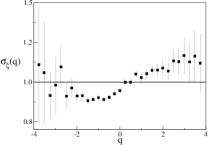
At the genome-wide level a further assumption of the Langevin equation (2) can be examined. There the noise amplitude was taken to be independent of the expression level $x$. To examine this assumption, the standard deviation $\sigma_{\xi}(q)$ of the noise term is computed at different rescaled expression levels $q$. Fig. 2(e) shows only an increase in noise variance of $15\%$ over the whole range of expression level changes. This increase of the noise amplitude may be due to increased experimental noise at higher expression levels, possibly arising from an intensity-dependent sensitivity of the fluorescence measurement of the microarrays. An alternative scenario for a changing noise-amplitude are stochastic fluctuations of the degradation rate $\eta$. However, such fluctuations would lead to a linear multiplicative noise term in the Langevin equation (2), that is, a noise amplitude which linearly increases with $q$. The saturation of $\sigma_{\xi}(q)$ at high and low values of $q$ which is seen in Fig. 2(e) does not support such a linear multiplicative scenario. This result – a small, nonlinear change in the noise amplitude – contradicts stochastic models with purely multiplicative noise which have been used in the literature [26, 27, 28].

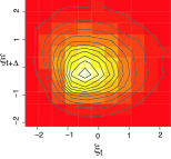
A last assumption behind the Langevin equation (2) and the corresponding propagator (2) is the statistical independence of noise terms at successive time steps. The distribution of successive noise terms $P(\xi_{t+\Delta},\xi_{t})$ across all genes is shown in Fig. 2(f). For small values of $\xi$, successive noise terms are independent, leading to circular contours in Fig. 2(f). For very short intervals $\Delta$ between measurements, not realised in currently available data, one should expect to find correlations between the noise terms $\xi(t)$ and $\xi(t+\Delta)$. Hence the assumption of uncorrelated noise will not hold for arbitrarily small sampling intervals. For this reason, the short term propagator (2) was used here, rather than the full propagator of an Ornstein-Uhlenbeck process with delta-correlated noise. In practice, this choice makes little difference for the results obtained.

These results show that the equation of motion (2) with an independent Gaussian distribution of noise of constant amplitude is a good description of the observed expression level dynamics. Some deviations occur at high and low expression levels. The origin of these deviations might, however, lie in the details of how the experiments [19] were taken. One particular source may be non-linearities in the relationship between expression levels and mRNA concentrations [20]. Future experiments, taken with different experimental technologies and at shorter sampling times, will allow further tests and possible modifications of the model.

3 mRNA degradation rates

We now discuss the biophysical parameters inferred from the expression level time courses of different genes. The decay times $\tau=\eta^{-1}$ inferred using (5) for different genes range from $350\mbox{s}$ to $9900\mbox{s}$ with mean $1400\mbox{s}$ and standard deviation $700\mbox{s}$. Decay times are found to differ somewhat across genes with different function, with mRNA of genes involved in transcription regulation being degraded faster than average ($\overline{\tau}=1200\pm 100\mbox{s}$), and those of genes involved in metabolic processes being degraded more slowly ($\overline{\tau}=1500\pm 50\mbox{s}$). A simple possible explanation for these different decay times is the need to quickly change concentrations of regulatory proteins in response to changing external conditions.

These results agree with experiments [29], where mRNA decay times were measured after halting mRNA production through a heat shock. (This unphysiological condition may well lead to different decay rates than under standard conditions.) The measured decay times range from $\tau=160\mbox{s}$ to $\tau=7800\mbox{s}$ with mean $1700\mbox{s}$ and standard deviation $560\mbox{s}$. The experimental study [29] also notes the relatively slow degradation of mRNA of genes involved in metabolic processes, and the faster degradation of those involved in regulatory systems.

4 Regulatory interactions

The transcription of genes is controlled by the presence of transcription factor proteins. Accordingly, the transcription rate $f$ of a target gene depends systematically on the concentration of its transcription factors. The dynamic equations of different genes are thus coupled by regulatory interactions. The resulting correlation of expression levels of different genes serves as the basis for exploring regulatory interactions.

We start by considering the effects of a single transcription factor on the mRNA concentration $x$ of a given gene. The key questions are (i) how does the transcription rate of a target gene depend on the concentration of its transcription factor and (ii) can one identify the targets of a given transcription factor from their effect on the transcription rate ? We generalize the stochastic dynamics (2) to

$$\partial_{t}x=-\eta x+f(y)+\sqrt{D/\Delta_{t}}\,\xi(t)\ ,$$ (6)

with the transcription rate $f(y)$ depending on the concentration $y$ of the transcription factor at time $t$. In the following, we will neglect post-transcriptional regulation and take the mRNA expression level of a transcription factor as a proxy for its protein concentration. The functional form of $f(y)$ for a given mRNA and a given transcription factor can be inferred by discretizing the continuous values of $y$ into a small number of bins containing an equal number of instances, and inferring the corresponding values of $f$ at the centres of these bins. An example, involving the transcription factor Swi4 and one of its targets, gene YN40, is shown in Fig. 3(a). Similar results are found for other transcription factors and their targets.

(a)

(b)

Figure 3: Transcription regulation by transcription factors. a) The functional form of the transcription rate $f(y)$ determined by discretizing the transcription factor expression levels $y$ into four bins with equal number of incidences and inferring the corresponding four values of the transcription rate $f$ (solid squares) along with the parameters $\eta$ and $D$. The result, shown here for transcription factor Swi4 and target YN40, agrees well with the Michaelis-Menten law (8) displayed by the solid line. Error bars indicate the point where the likelihood (4) has decayed to $e^{-1/2}$ of its maximum, corresponding approximately to one standard deviation. b) The distribution of binding energies (relative to their free energies in solution) of the Swi4–DNA and the Swi4–Swi6 interactions, see text.

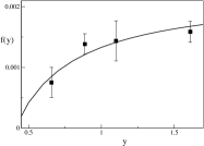
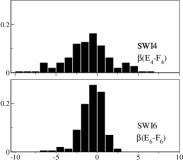
Fig. 3(a) displays a non-linear relationship between transcription factor concentration and the target transcription rate showing saturation at high concentrations. This is expected since at high transcription factor concentration most binding sites are occupied by a transcription factor molecule, and further increases of concentration no longer have a strong effect. Assuming that a transcription factor may either be bound at a binding site, or be suspended in solution or bound non-specifically elsewhere on DNA, the probability of a given site being occupied is given by elementary statistical mechanics [30] as

$$P(y)=\frac{ye^{-\beta E}}{ye^{-\beta E}+e^{-\beta F}}$$ (7)

and depends on the transcription factor concentration $y$, binding energy $E$ and a free energy $F$ of the transcription factor in solution or bound elsewhere.

Assuming the transcription rate to depend linearly on the probability that the binding site is occupied at a given time one obtains

$$f(y)=f_{0}+\delta P(y)\ ,$$ (8)

where $f_{0}$ is a basal transcription rate in the absence of transcription factors and $\delta$ quantifies the change of the transcription rate due to transcription factor binding. Positive values of $\delta$ describe enhancers and negative values of $\delta$ indicate repressors. The functional form (8) is the celebrated Michaelis-Menten kinetics, first studied in the context of enzymatic reactions nearly a century ago [31] and used widely in transcription modelling [14]. Like many other targets of transcription factor Swi4, the relationship between transcription rate of target YN40 and transcription factor concentration fits the Michaelis-Menten model well, see Fig. 3(a).

One can turn this result on its head and use the Michaelis-Menten model (8) and equations (5) – (6) to infer the binding parameters $\beta(E-F),f_{0},\delta$ of a transcription factor for different genes. We expect that genes with a high response $\Delta f\equiv f(y_{\max})-f(y_{\min})$ to changes in concentration of a transcription factor are targets of that transcription factor. We test this relationship for the transcription factor Swi4, and consider genes with different number of Swi4 binding sequences in their regulatory region, see Figure 4. One finds that $\Delta f$ tends to increase with the number of binding sequences, indicating that Swi4 acts an enhancer of gene expression. The $10$ genes with the highest $\Delta f$ are CDC9, RNR1, YG3N, CRH1, YIO1, RAD27, PRY2, CSI2, PMS5, and CDC21. With a single exception, all of these genes have at least one copy of the Swi4 binding sequence in their regulatory region. Furthermore, $8$ of the $10$ predicted targets have been previously found experimentally [32].

Figure 4: Genes with a higher number of Swi4 binding sites respond more strongly to changes in the Swi4 expression level. The distribution of the range $\Delta f\equiv|f(y_{\max})-f(y_{\min})|$ of the force term is shown for different sets of genes: all genes (black), genes with one or more Swi4 binding motifs (red), genes with two or more motifs (green), genes with three or more Swi4 binding motifs (blue). Genes with a higher number of binding sites are seen to have a larger amplitude of the driving force.

Many genes are regulated by more than one transcription factor. Higher organisms in particular owe much of their complexity to the combinatorial logic implemented by the cooperative binding of several transcription factors [33]. For instance, the transcription factor Swi4 forms a dimer with transcription factor Swi6, with Swi4 binding to regulatory DNA and Swi6 attracting the polymerase molecule which starts transcription [34], see Fig. 1(a). For this situation, the binding probability (7) generalizes to

$$P(y_{4},y_{6})=\frac{y_{4}y_{6}}{e^{\beta(E_{4}-F_{4}+E_{6}-F_{6})}+y_{4}e^{\beta(E_{6}-F_{6})}+y_{4}y_{6}}\ ,$$ (9)

where $y_{4}$ and $y_{6}$ are the concentrations of Swi4 and Swi6, respectively. The constant $E_{4}$ gives the energy of Swi4–DNA binding and $F_{4}$ the free energy of Swi4 in solution, $E_{6}$ is the energy of the Swi4–Swi6 interaction and $F_{6}$ the free energy of Swi6 in solution. The Swi4–DNA energy depends on the binding sequence in the regulatory region of a given gene and may thus vary from gene to gene. On the other hand, the Swi4–Swi6 interaction does not depend on the target gene. Fig. 3(b) shows the distribution of ${\beta(E_{4}-F_{4})}$ and ${\beta(E_{6}-F_{6})}$ inferred by maximum likelihood for different targets of Swi4–Swi6. As expected, the variance of the Swi4–Swi6 interaction is significantly smaller than that of the Swi4–DNA interaction.

5 Discussion

Some of the properties of gene expression are likely to be universal and occur in many organisms under many circumstances. An example is the biophysical implementation of transcription regulation through the binding of molecules, with the resulting saturation of bound molecules at high concentrations. Another is the independent degradation of mRNA molecules, leading to the linear drift of mRNA concentrations. (This is less universal, since at very high concentrations mRNA molecules may outnumber RNase molecules responsible for mRNA degradation.)

Other properties of gene expression are specific to a given organism. Indeed, higher organisms, which share largely the same set of genes, derive most of their diversity from specific changes in how those genes are regulated [35]. These specific properties include the transcription factor binding sites in the regulatory region of a gene, and the interactions between transcription factors. In this paper we have used simple stochastic models of mRNA dynamics based on the universal properties to infer some of the specific properties of gene expression in yeast. Current and future developments in molecular biology will bring dynamically resolved data on other types of molecules apart from messenger RNA: concentrations of regulatory proteins themselves [36, 25] or of $\mu$RNA, which silences specific mRNA molecules, leading to new challenges in the non-equilibrium dynamics of genetic regulation.

6 Appendix

The mRNA expression data of Spellman [19] comprises four time courses corresponding to different ways of synchronizing yeast cell cultures to the same phase in the cell cycle. Three timecourses were used here (termed alpha, cdc15, cdc28 in [19]), each set equally contributing to the likelihood (4). These different timecourses correspond to different ways of synchronizing a population of cells in a given phase of the cell cycle. The fourth set (elu) was not used as it systematically lead to decreased likelihoods in (4). The likelihood (4) also allows to identify probes on the chip which give results compatible with uncorrelated random data; only probes where (4) gave log-likelihoods larger than $1.1$ the log-likelihood of the data under an uncorrelated Gaussian model were used. Set alpha contains $18$ samples spaced $7$ minutes apart, cdc15 $24$ samples $10-20$ minutes apart, cdc28 contains $17$ samples spaced $10$ minutes apart.

The functional classification of genes followed the Gene Ontology [37] using the terms transcription regulation activity (GO:0030528) and metabolic process (GO:0008152).

The canonical binding sequence for Swi4 is “CRCGAAA” where R stands for either G or A [38]. Regions $500$ base pairs before the transcription initiation point were searched for copies of this sequence (or its reverse, its complement, or its reverse complement) . Sequences were taken from www.ncbi.nlm.nih.gov/CBBresearch/Landsman/Cell_ cycle_data/upstream_seq.html $24\%$ of all yeast genes contain at least one copy of the Swi4 binding sequence in their regulatory region, $4\%$ contain two copies or more. The yeastract-database [32] list $170$ Swi4 targets verified experimentally, or about $3\%$ of the yeast genes.

The example gene YN40 in Figs. 2 and 3(a) was chosen due to the high number of $3$ Swi4 binding sites within $500$ basepairs and $5$ sites within $1000$ basepairs of the transcription initiation site.